
Recommended
More Related Content
What's hot
What's hot (20)
Similar to ilovepdf_merged
Similar to ilovepdf_merged (20)
ilovepdf_merged
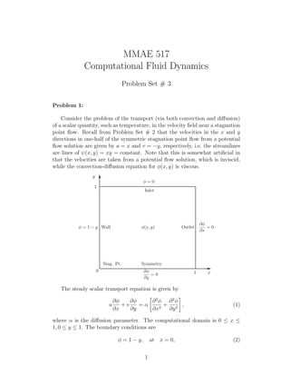
- 1. MMAE 517 Computational Fluid Dynamics Problem Set # 3 Problem 1: Consider the problem of the transport (via both convection and diffusion) of a scalar quantity, such as temperature, in the velocity field near a stagnation point flow. Recall from Problem Set # 2 that the velocities in the x and y directions in one-half of the symmetric stagnation point flow from a potential flow solution are given by u = x and v = −y, respectively, i.e. the streamlines are lines of ψ(x, y) = xy = constant. Note that this is somewhat artificial in that the velocities are taken from a potential flow solution, which is inviscid, while the convection-diffusion equation for φ(x, y) is viscous. ∂φ ∂y = 0 OutletWall Inlet Stag. Pt. 1 y x0 Symmetry φ(x, y) φ = 0 1 ∂φ ∂x = 0φ = 1 − y The steady scalar transport equation is given by u ∂φ ∂x + v ∂φ ∂y = α ∂2 φ ∂x2 + ∂2 φ ∂y2 , (1) where α is the diffusion parameter. The computational domain is 0 ≤ x ≤ 1, 0 ≤ y ≤ 1. The boundary conditions are φ = 1 − y, at x = 0, (2) 1
- 2. ∂φ ∂x = 0, at x = 1, (3) ∂φ ∂y = 0, at y = 0, (4) φ = 0, at y = 1, (5) Modify your ADI algorithm from Problem Set # 2 to include upwind-downwind differencing of the convective terms on the left-hand-side of equation (1). Look- ing ahead to Problem Set # 4, do not assume that u > 0 and v < 0. Obtain grid independent solutions for φ(x, y) with values of α equal to 0.1 and 0.01. Note that you may need to use a different convergence criterion and/or ac- celeration parameters as compared to problem set #2. In addition, different values of α may require different acceleration parameters. 2
- 3. Marcello de Oliveira Gomes MMAE 517 PROBLEM SET #3 The goal of this problem set is to solve the steady scalar equation with the following boundary conditions ݑ ∂ϕ ∂x + ݒ ߲߶ ߲ݔ = ߙ[ ߲ଶ ߶ ߲ݔଶ + ߲ଶ ߶ ߲ݕଶ ] Solution will use upwind and downwind differencing in an ADI code similar to the one used in problem set #2. Some improvements from the last code include a better way of determining the parameters for Thomas call. Instead of a for loop calculating each single value of a,b, c, and d, matrix multiplication is applied throughout the entire line or column. This makes the code run about 10% faster. Left and top boundaries are defined before calling the upwind/downwind function and are not iterated inside it. Approximation is done by using central difference on the diffusion terms and forward or backward difference on the convective terms, depending on u and v sign. For u>0 ߙ߶ାଵ, − ൫ݑ,Δݔ + 2ߙ൯߶, + ൫ߙ + ݑ,Δݔ൯߶ିଵ, [1]
- 4. For u<0 ൫ߙ − ݑ,Δݔ൯߶ାଵ, − ൫−ݑ,Δݔ + 2ߙ൯߶, + ߙ߶ିଵ, [2] For v>0 Δഥ[−ߙΔഥ߶,ାଵ + ൫2ߙΔഥ + ݒ,Δݔ൯߶, − ൫ߙΔഥ + Δݒݔ,൯߶,ିଵ [3] For v<0 Δഥ[൫−ߙΔഥ + Δݒݔ,൯߶,ାଵ + ൫2ߙΔഥ − ݒ,Δݔ൯߶, − ߙΔഥ߶,ିଵ] [4] The acceleration parameter,ߪ, should be inserted inside ߶, brackets in both sides of the equations. If sweeping across constant lines, Thomas parameters a,b, and c will be the ones for u>0 or u<0. In this case, −ߪ߶, should be inserted in both sides of the equation. For u>0 and v<0 and sweeping in constant y lines the equation should look like the following. ߙ߶ାଵ, − ൫ݑ,Δݔ + 2ߙ + ߪ൯߶, + ൫ߙ + ݑ,Δݔ൯߶ିଵ, = Δഥ[൫−ߙΔഥ + Δݒݔ,൯߶,ାଵ + ቀ2ߙΔഥ + ݒ,Δݔ − ఙ ഥ ቁ ߶, − ߙΔഥ߶,ିଵ] [5] Boundary conditions are treated as usual. For this problem left and top boundaries are Dirichlet and do not need to be iterated. Treatment of right and bottom results in the following equations. For i=I and for u>0 −൫ݑ,Δݔ + 2ߙ − ߪ൯߶, + ൫2ߙ + ݑ,Δݔ൯߶ିଵ, [6] For j=1 and v<0 Δഥ[൫−2ߙΔഥ + Δݒݔ,൯߶,ାଵ + ൫2ߙΔഥ + ݒ,Δݔ − ߪ൯߶, − ߙΔഥ߶,ିଵ] [7] Best value for the parameter ߪ is found by iterating solution in a 11x11 mesh and kept as being the one which returns the lowest number of iterations. Considering an error of 10ିସ for ADI iterations is a major mistake leading to fast convergence, returning a very small number of iterations and wrong solutions for the problem as shown in Figure 1. Decreasing grid size only diverges solution, making the right boundary approach zero
- 5. for a mesh of 501x501 (in this case, new phi zero matrix was defined for each iteration, leading to the approximation of zero value for right boundary condition). Real best value that suits both ߙ was found to be around ߪ =0.2 for error of 10ି . Figure 1 - Solution for sigma =0.18 and error = 10^-4 in 50x50 and 301x301 mesh Figure 2 - Sigma values x needed iterations Grid independent solution was determined by inspecting maximum difference between 121 fixed points in the domain. Even though maximum difference is expected to happen between right and bottom boundaries, convergence code was kept this way for future uses, contemplating more general cases. Initial matrix had a size of 51x51, and increased linearly up to the point where error between solutions was 1%. Though, every time matrix increases the last solution was used to populate new matrix phi. This way, instead of reaching solution from zero matrixes, code will use previous solution,
- 6. reducing computation time in more than half. Although it is already a great gain, this approach still can be further improved for faster solutions. Scheme is show in Figure 3 Figure 3 - Solution reutilization By inspections of the boundaries, left side of the domain is a straight line starting at y=1 and ending at y=0, while top is x =0, Figure 4 and Figure 5, which confirms boundary conditions given in the problem. As can be noted by comparison, solution does not vary significantly. Maximum error between solutions was found to be 0.0072 and 0.0051 with grid independent solutions of 101x101 and 151x151 for ߙ values of 0.1 and 0.01 respectively. Iteration time for ߙ equals to 0.1 and 0.01 were 37s and 518s respectively. Figure 4 - Solution for ࢻ= 0.1, 51x51 mesh
- 7. Figure 5 - Solution for ࢻ= 0.1, 101x101 mesh Figure 6 – Constant streamlines ࢻ = .
- 8. Figure 7 - Solution for ࢻ = 0.01, 151x151 mesh Figure 8 - Constant streamlines ࢻ=0.01 Backward and forward approximations bring the truncation error of the solution to the order of Δ.ݔ An estimative of the true ߙ value that is being calculated can be taken by equation 8. Variation of ߙ with grid size is shown in Figure 9 ߙ = ߙ − ௫ ଶ [8]
- 9. Figure 9-Real alpha due to upwind/downwind approximation Figure 9 shows that to obtain an error of only 5% in ߙ values for maximum velocity it is needed a mesh size of 101x101 and 1001x1001 for ߙ = 0.1 and 0.01 respectively. This task is doable for 101 points in each direction but not for a 1001. Computation time gets extremely long and code tends to be not viable anymore when bigger problems are concerned. 0 5 10 15 20 25 30 35 40 45 50 0 200 400 600 800 1000 Differencein% Mesh size (NxN) alpha = 0.1 alpha=0.01
- 10. Main Code clear all clc error = 10^-6; % error for ending iteration alpha = 0.1; sigma = 0.2; cnt = 5; %this variable will increase grid size compare = zeros(11,11,2); A = zeros(50,50); % this matrix will store results for 50x50 max_dif = 5; %just a random large number BC1=0; BC2 = 0; figure(1) hold on grid on while max_dif>10^-2 I = (cnt*10)+1; J = (cnt*10)+1; delta_x = 1/(I-1); delta_y = 1/(J-1); y = (0:delta_y:1); %vector containing y positions x = (0:delta_x:1); u= zeros(I,J); v = zeros(I,J); %ALL THE COMMENTS INSIDE THIS BOX ARE FOR DETERMINING BEST SIGMA VALUE----- % figure(1) % grid on % hold on % sigma = (1.1:0.01:1.2); %what's best value for sigma??? n_min=10^15; %minimum number of iterations. Set to be a high value to avoid problems %determining best value of sigma % for z=1:size(sigma,2) phi = zeros(I,J); for i=1:cnt/5 for j=1:cnt/5 phi((i-1)*size(A,2)+1:size(A,2)*i,(j- 1)*size(A,2)+1:size(A,2)*j)= A; end end for i=1:J phi(1,i) = 1- y(i); u(i,:) = delta_x*(i-1); end for i=1:I phi(i,I) = 0; v(:,i) = -delta_y*(i-1); end left = [1 0 0; 0 1 0]; %since left boundary for x is dependenton y, it will be taken in account inside upwing code. right = [0 1 0; 1 0 0]; tic
- 11. [phi,N] = updown_wind_tentative(alpha,phi,I,J,u,v,delta_x,delta_y,error,sigma,BC 1,BC2,left,right); A = phi(1:50,1:50); % if isnan(phi) %this if checks if any of phi values are NaN % N=0; % end % % if N<n_min && N~=0 %keeping fastest sigma % n_min=N; % value = z; %stores when minimum number of iterations happened % end % plot(sigma(z),N,'dk') % fprintf('iteration %dn',z) % % end % % xlabel('Sigma','FontSize',13) % ylabel('Number of Iterations','FontSize',13) % title('Sigma x Number of Iterations','FontSize',17) % hold off % end % ###################################################################### ### %--------------------------------------------------------------------- ----- %For checking convergence, uncomment this section and while on line 19 plot(I,max_dif,'dk') [max_dif,compare]= convergence(compare,phi,cnt); xlabel('Grid size','FontSize',13) ylabel('Maximum error','FontSize',13) title('Error between previous and current solution','FontSize',17) cnt = cnt+5; end time = toc hold off figure(2) mesh(x,y,phi) title('3-D phi') xlabel('X') ylabel('Y') zlabel('PHI') figure(3) hold on grid on contour(x,y,phi','ShowText','on') title('Constant streamlines') xlabel('X') ylabel('Y') hold off % %-------------------------------------------------------------------
- 12. updown_wind_tentative % I is the number of nodes in x direction % J is the number of nodes in y direction % sigma is the acceleration parameter % error is the minimum acceptable difference between iterations % u is the velocity vector, size IxJ % v is the velocity vector, size IxJ % BC1 is the value for the Neumann boundary condition on the right side % BC2 is the bottom boundary condition % left and right are the boundary conditions as specified in Thomas -> % First line indicates X(constant j lines) and second line indicates % Y(constant i lines) function [phi,n_iterations] = updown_wind_tentative(alpha,phi,I,J,u,v,delta_x,delta_y,error,sigma,BC 1,BC2,left,right) % %Defining parameters leftx = left(1,:); lefty = left(2,:); rightx = right(1,:); righty = right(2,:); delta_bar = (delta_x/delta_y); % ATTENTION it is defined differently here!!!!!! er_max = 2; %random value n_iterations=0; %counter a = zeros(I,1); b = zeros(I,1); c = zeros(I,1); d = zeros(I,1); old_value = zeros(1,J); while er_max>=error er_max = 0; %sweeping across constant j lines %phi values will be stored as matrix collumns j = 1; b(:,1) = -(abs(u(:,j)*delta_x)+ 2*alpha+sigma); a(:,1) = u(:,j)*delta_x+alpha; c(:,1) = alpha; d(:,1)= delta_bar*((-v(:,j)*delta_x+2*alpha*delta_bar - sigma/delta_bar).*phi(:,j) +(v(:,j)*delta_x- 2*alpha*delta_bar).*phi(:,j+1)+2*alpha*delta_bar*delta_y*BC1); leftx(1,3)= 1-delta_y*(j-1); test = thomas(I-1,delta_x,a,b,c,d,leftx,rightx); phi(:,j) = test; for j=2:J-1 %Dirichlet boundary at j=J is not iterated b(:,1) = -(abs(u(:,j)*delta_x)+ 2*alpha+sigma); a(:,1) = u(:,j)*delta_x+alpha; c(:,1) = alpha; d(:,1)= delta_bar*((-v(:,j)*delta_x+2*alpha*delta_bar - sigma/delta_bar).*phi(:,j) -alpha*delta_bar.*phi(:,j-1) +(v(:,j)*delta_x-alpha*delta_bar).*phi(:,j+1)); %fixing boundary condition, dependence on y! leftx(1,3)= 1-delta_y*(j-1); test = thomas(I-1,delta_x,a,b,c,d,leftx,rightx); phi(:,j) = test; end %---------------------------------------------------------------------
- 13. %phi values will be stored as matrix lines for i=2:I-1 old_value(1,:) = phi(i,:); b(:,1) = delta_bar*((abs(v(i,:)*delta_x)+2*alpha*delta_bar + sigma/delta_bar)); a(:,1) = -alpha*delta_bar^2; c(:,1) = delta_bar*(v(i,:)*delta_x-alpha*delta_bar); d(:,1)= -(u(i,:)*delta_x+2*alpha-sigma).*phi(i,:)+ (u(i,:)*delta_x+alpha).*phi(i-1,:)+alpha.*phi(i+1,:); %thomas returns a collumn vector. It has to be fixed before assigning it to phi test = thomas(J-1,delta_y,a,b,c,d,lefty,righty);%temporary variable to store results phi(i,:) = test(:,1); er_point = max(abs(phi(i,:)- old_value))/max(max(abs(phi)));%maximum error in constant i line if er_point>er_max er_max = er_point; end end i=I; old_value(1,:) = phi(i,:); b(:,1) = delta_bar*((abs(v(i,:)*delta_x)+2*alpha*delta_bar + sigma/delta_bar)); a(:,1) = -alpha*delta_bar^2; c(:,1) = delta_bar*(v(i,:)*delta_x-alpha*delta_bar); d(:,1) = -(u(i,:)*delta_x+2*alpha-sigma).*phi(i,:)+ (u(i,:)*delta_x+2*alpha).*phi(i-1,:)+2*alpha*BC2*delta_x; test = thomas(J-1,delta_y,a,b,c,d,lefty,righty);%temporary variable to store results phi(i,:) = test(:,1); er_point = max(abs(phi(i,:)-old_value))/max(max(abs(phi)));%maximum error in constant i line if er_point>er_max er_max = er_point; end n_iterations=n_iterations+1; end end