SlideShare a Scribd company logo
1 of 50
Download to read offline
SEDRA-ISM: “E-CH04” — 2014/11/12 — 11:02 — PAGE 1 — #1
Exercise 4–1
Ex: 4.1 Refer to Fig. 4.3(a). For vI ≥ 0, the
diode conducts and presents a zero voltage drop.
Thus vO = vI . For vI < 0, the diode is cut off,
zero current flows through R, and vO = 0. The
result is the transfer characteristic in Fig. E4.1.
Ex: 4.2 See Fig. 4.3a and 4.3b. During the
positive half of the sinusoid, the diode is forward
biased, so it conducts resulting in vD = 0. During
the negative half cycle of the input signal vI , the
diode is reverse biased. The diode does not
conduct, resulting in no current flowing in the
circuit. So vO = 0 and vD = vI − vO = vI . This
results in the waveform shown in Fig. E4.2.
Ex: 4.3 ˆiD =
ˆvI
R
=
10 V
1 k
= 10 mA
dc component of vO =
1
π
ˆvO
=
1
π
ˆvI =
10
π
= 3.18 V
Ex: 4.4
(a)
ϩ5 V
V ϭ 0 V
ϭ 2 mAI ϭ2.5 k⍀
5 Ϫ 0
2.5
ϩ
Ϫ
(b)
ϩ5 V
V ϭ 5 V
I ϭ 0 A2.5 k⍀
ϩ
Ϫ
(c)
Ϫ5 V
V ϭ 5 V
I ϭ 0 A
ϩ
Ϫ
2.5 k⍀
(d)
Ϫ5 V
V ϭ 0 V
0 ϩ 5
2.5
I ϭ
ϩ
Ϫ
2.5 k⍀ϭ 2 mA
(e)
V ϭ 3 V
3 V
2 V
1 V
3
1
I ϭ1 k⍀ ϭ 3 mA
0
0
I
(f)
ϩ3 V
ϩ2 V
ϩ1 V
I ϭ1 k⍀
ϩ5 V
0
0
I
V ϭ 1 V
ϭ 4 mA
5 Ϫ 1
1
ϩ
Ϫ
Ex: 4.5 Vavg =
10
π
50 + R =
10
π
1 mA
=
10
π
k
∴ R = 3.133 k
SEDRA-ISM: “E-CH04” — 2014/11/12 — 11:02 — PAGE 2 — #2
Exercise 4–2
Ex: 4.6 Equation (4.5)
V2 − V1 = 2.3 VT log
I2
I1
At room temperature VT = 25 mV
V2 − V1 = 2.3 × 25 × 10−3
× log
10
0.1
= 115 mV
Ex: 4.7 i = IS ev/VT
(1)
1 (mA) = IS e0.7/VT
(2)
Dividing (1) by (2), we obtain
i (mA) = e(v−0.7)/VT
⇒ v = 0.7 + 0.025 ln(i)
where i is in mA. Thus,
for i = 0.1 mA,
v = 0.7 + 0.025 ln(0.1) = 0.64 V
and for i = 10 mA,
v = 0.7 + 0.025 ln(10) = 0.76 V
Ex: 4.8 T = 125 − 25 = 100◦
C
IS = 10−14
× 1.15 T
= 1.17 × 10⁻⁸
A
Ex: 4.9 At 20◦
C I =
1 V
1 M
= 1 μA
Since the reverse leakage current doubles for
every 10◦
C increase, at 40◦
C
I = 4 × 1 μA = 4 μA
⇒ V = 4 μA × 1 M = 4.0 V
@ 0◦
C I =
1
4
μA
⇒ V =
1
4
× 1 = 0.25 V
Ex: 4.10 a. Use iteration:
Diode has 0.7 V drop at 1 mA current.
Assume VD = 0.7 V
ID =
5 − 0.7
10 k
= 0.43 mA
Use Eq. (4.5) and note that
V1 = 0.7 V, I1 = 1 mA
ID
VCC
ϭ 5 V VD
R ϭ 10 k⍀
ϩ
Ϫ
V2 − V1 = 2.3 × VT log
I2
I1
V2 = V1 + 2.3 × VT log
I2
I1
First iteration
V2 = 0.7 + 2.3 × 25 × 10−3
log
0.43
1
= 0.679 V
Second iteration
I2 =
5 − 0.679
10 k
= 0.432 mA
V2 = 0.7 + 2.3 × 25.3 × 10−3
log
0.432
1
= 0.679 V 0.68 V
we get almost the same voltage.
∴ The iteration yields
ID = 0.43 mA, VD = 0.68 V
b. Use constant voltage drop model:
VD = 0.7 V constant voltage drop
ID =
5 − 0.7
10 k
= 0.43 mA
Ex: 4.11
RI
10 V
2.4 V
ϩ
Ϫ
Diodes have 0.7 V drop at 1 mA
∴ 1 mA = IS e0.7/VT
(1)
At a current I(mA),
I = IS eVD/VT
(2)
Using (1) and (2), we obtain
I = e(VD−0.7)/VT
SEDRA-ISM: “E-CH04” — 2014/11/12 — 11:02 — PAGE 3 — #3
Exercise 4–3
For an output voltage of 2.4 V, the voltage drop
across each diode =
2.4
3
= 0.8 V
Now I, the current through each diode, is
I = e(0.8−0.7)/0.025
= 54.6 mA
R =
10 − 2.4
54.6 × 10−3
= 139
Ex: 4.12
(a)
ϩ5 V
V ϭ 0.7 V
I ϭ ϭ 1.72 mA2.5 k⍀
5 Ϫ 0.7
2.5
ϩ
Ϫ
(b)
ϩ5 V
V ϭ 5 V
I ϭ 0 A 2.5 k⍀
ϩ
Ϫ
(c)
Ϫ5 V
V ϭ 5 V
I ϭ 0 A
ϩ
Ϫ
2.5 k⍀
(d)
Ϫ5 V
Ϫ0.7 ϩ 5
2.5
I ϭ
ϩ
Ϫ
2.5 k⍀
ϭ 1.72 mA
V ϭ 0.7 V
(e)
V ϭ 3 Ϫ 0.7
3 V
2 V
1 V
2.3
1
I ϭ
I
0
0
1 k⍀
ϭ 2.3 mA
ϭ 2.3 V
(f)
ϩ3 V
0
ϩ2 V
ϩ1 V
I ϭ
1 k⍀
5 V
0
I
V ϭ 1 ϩ 0.7
ϭ 1.7 V
ϭ 3.3 mA
5 Ϫ 1.7
1
Ex: 4.13 rd =
VT
ID
ID = 0.1 mA rd =
25 × 10−3
0.1 × 10−3
= 250
ID = 1 mA rd =
25 × 10−3
1 × 10−3
= 25
ID = 10 mA rd =
25 × 10−3
10 × 10−3
= 2.5
Ex: 4.14 For small signal model,
iD = vD/rd (1)
where rd =
VT
ID
For exponential model,
iD = IS eV/VT
SEDRA-ISM: “E-CH04” — 2014/11/12 — 11:02 — PAGE 4 — #4
Exercise 4–4
iD2
iD1
= e(V2−V1) /VT = e vD/VT
iD = iD2 − iD1 = iD1e vD /VT − iD1
= iD1 e vD/VT − 1 (2)
In this problem, iD1 = ID = 1 mA.
Using Eqs. (1) and (2) with VT = 25 mV, we
obtain
vD (mV) iD (mA) iD (mA)
small exponential
signal model
a − 10 − 0.4 − 0.33
b − 5 − 0.2 − 0.18
c + 5 + 0.2 + 0.22
d + 10 + 0.4 + 0.49
Ex: 4.15
R
IL
VO
ϩ15 V
a. In this problem,
VO
iL
=
20 mV
1 mA
= 20 .
∴ Total small-signal resistance of the four diodes
= 20
∴ For each diode, rd =
20
4
= 5 .
But rd =
VT
ID
⇒ 5 =
25 mV
ID
.
∴ ID = 5 mA
and R =
15 − 3
5 mA
= 2.4 k .
b. For VO = 3 V, voltage drop across each diode
=
3
4
= 0.75 V
iD = IS eV/VT
IS =
iD
eV/VT
=
5 × 10⁻³
e0.75/0.025
= 4.7 × 10⁻¹⁶
A
c. If iD = 5 − i L = 5 − 1 = 4 mA.
Across each diode the voltage drop is
VD = VT ln
ID
IS
= 25 × 10−3
× ln
4 × 10⁻³
4.7 × 10−16
= 0.7443 V
Voltage drop across 4 diodes
= 4 × 0.7443 = 2.977 V
so change in VO = 3 − 2.977 = 23 mV.
Ex: 4.16 For a zener diode
VZ = VZ0 + IZ rZ
10 = VZ0 + 0.01 × 50
VZ0 = 9.5 V
For IZ = 5 mA,
VZ = 9.5 + 0.005 × 50 = 9.75 V
For IZ = 20 mA,
VZ = 9.5 + 0.02 × 50 = 10.5 V
Ex: 4.17
IR
15 V
5.6 V
0 to 15 mA
The minimum zener current should be
5 × IZk = 5 × 1 = 5 mA
Since the load current can be as large as 15 mA,
we should select R so that with IL = 15 mA, a
zener current of 5 mA is available. Thus the
current should be 20 mA, leading to
R =
15 − 5.6
20 mA
= 470
Maximum power dissipated in the diode occurs
when IL = 0 is
Pmax = 20 × 10−3
× 5.6 = 112 mV
SEDRA-ISM: “E-CH04” — 2014/11/12 — 11:02 — PAGE 5 — #5
Exercise 4–5
Ex: 4.18
15 V
200 ⍀
Thus, at no load VZ 5.1 V
ϩ
Ϫ
VZ
15 Ϫ 5.1
0.2 k⍀
I ϭ ϭ 49.5 mA
50 mA
For line regulation:
200 ⍀
7 ⍀vi
vo
Ϫϩ
Line regulation =
vo
vi
=
7
200 + 7
= 33.8
mV
V
For load regulation:
200 ⍀
VZ0
VO
rZ
⌬IL
VO
IL
=
− IL(rZ 200 )
IL mA
= −6.8
mV
mA
Ex: 4.19
␲
vS
VD
2␲
␻t
Vs ϭ 12 2
0
uu
a. The diode starts conduction at
vS = VD = 0.7 V
vS = Vs sin ωt, here Vs = 12
√
2
At ωt = θ,
vS = Vs sin θ = VD = 0.7 V
12
√
2 sin θ = 0.7
θ = sin−1 0.7
12
√
2
2.4◦
Conduction starts at θ and stops at 180 − θ.
∴ Total conduction angle = 180 − 2θ = 175.2◦
b. vO,avg =
1
2π
(π−θ)
θ
(Vs sin φ − VD) dφ
=
1
2π
[−Vs cos φ − VDφ]φ=π−θ
φ−θ
=
1
2π
[Vs cos θ − Vs cos (π − θ) − VD (π − 2θ)]
But cos θ 1, cos (π − θ) − 1, and
π − 2θ π
vO,avg =
2Vs
2π
−
VD
2
=
Vs
π
−
VD
2
For Vs = 12
√
2 and VD = 0.7 V
vO,avg =
12
√
2
π
−
0.7
2
= 5.05 V
c. The peak diode current occurs at the peak
diode voltage.
∴ ˆiD =
Vs − VD
R
=
12
√
2 − 0.7
100
= 163 mA
PIV = +VS = 12
√
2
17 V
Ex: 4.20
( )
␪
␪␲
vS
Vs
ϪVS
Ϫ
␪␲ ϩVD
output
0
input
␻t
a. As shown in the diagram, the output is zero
between (π − θ) to (π + θ)
= 2θ
SEDRA-ISM: “E-CH04” — 2014/11/12 — 11:02 — PAGE 6 — #6
Exercise 4–6
Here θ is the angle at which the input signal
reaches VD.
∴ Vs sin θ = VD
θ = sin−1 VD
Vs
2θ = 2 sin−1 VD
Vs
b. Average value of the output signal is given by
VO =
1
2π
⎡
⎣2 ×
(π−θ)
θ
(Vs sin φ − VD) dφ
⎤
⎦
=
1
π
[−Vs cos φ − VDφ]π−θ
φ=θ
2
Vs
π
− VD, for θ small.
c. Peak current occurs when φ =
π
2
.
Peak current
=
Vs sin (π /2) − VD
R
=
Vs − VD
R
If vS is 12 V(rms),
then Vs =
√
2 × 12 = 12
√
2
Peak current =
12
√
2 − 0.7
100
163 mA
Nonzero output occurs for angle = 2 (π − 2θ)
The fraction of the cycle for which vO > 0 is
=
2 (π − 2θ)
2π
× 100
=
2 π − 2 sin−1 0.7
12
√
2
2π
× 100
97.4 %
Average output voltage VO is
VO = 2
Vs
π
− VD =
2 × 12
√
2
π
− 0.7 = 10.1 V
Peak diode current ˆiD is
ˆiD =
Vs − VD
R
=
12
√
2 − 0.7
100
= 163 mA
PIV = Vs − VD + VS
= 12
√
2 − 0.7 + 12
√
2
= 33.2 V
Ex: 4.21
Vs
ϪVs
ϭ sin–1
΂ ΃
2VD
output
0
2VD
VS
input
␪
t
(a) VO,avg =
1
2π
(Vs sin φ − 2VD) dφ
=
2
2π
[−Vs cos φ − 2VDφ]π−θ
φ=θ
=
1
π
[Vs cos φ − Vs cos(π − θ) − 2VD(π − 2θ)]
But cos θ ≈ 1,
cos (π − θ) ≈ − 1
π − 2θ ≈ π. Thus
⇒ VO,avg
2Vs
π
− 2VD
=
2 × 12
√
2
π
− 1.4 = 9.4 V
(b) Peak diode current =
Peak voltage
R
=
Vs − 2VD
R
=
12
√
2 − 1.4
100
= 156 mA
PIV = Vs − VD = 12
√
2 − 0.7 = 16.3 V
Ex: 4.22 Full-wave peak rectifier:
R C
ϩ
Ϫ
vO
vS
ϩ
Ϫ
vS
D1
D2
Vp
Vr
assume
ideal diodes
t
⌬t
{
T
2
The ripple voltage is the amount of voltage
reduction during capacitor discharge that occurs
SEDRA-ISM: “E-CH04” — 2014/11/12 — 11:02 — PAGE 7 — #7
Exercise 4–7
when the diodes are not conducting. The output
voltage is given by
vO = Vpe−t/RC
Vp − Vr = Vpe− T/2
RC ← discharge is only half
the period. We also assumed t
T
2
.
Vr = Vp 1 − e− T/2
RC
e− T/2
RC 1 −
T/2
RC
, for CR T/2
Thus Vr Vp 1 − 1 +
T/2
RC
Vr =
Vp
2fRC
(a) Q.E.D.
To find the average diode current, note that the
charge supplied to C during conduction is equal
to the charge lost during discharge.
QSUPPLIED = QLOST
iCav t = CVr SUB (a)
iD,av − IL t = C
Vp
2fRC
=
Vp
2fR
=
Vpπ
ωR
iD,av =
Vpπ
ω tR
+ IL
where ω t is the conduction angle.
Note that the conduction angle has the same
expression as for the half-wave rectifier and is
given by Eq. (4.30),
ω t ∼=
2Vr
Vp
(b)
Substituting for ω t, we get
⇒ iD,av =
πVp
2Vr
Vp
· R
+ IL
Since the output is approximately held at Vp,
Vp
R
≈ IL · Thus
⇒ iD,av
∼= πIL
Vp
2Vr
+ IL
= IL 1 + π
Vp
2Vr
Q.E.D.
If t = 0 is at the peak, the maximum diode current
occurs at the onset of conduction or at t = −ω t.
During conduction, the diode current is given by
iD = iC + iL
iD,max = C
dvS
dt t=−ω t
+ iL
assuming iL is const. iL
Vp
R
= IL
= C
d
dt
Vp cos ωt + IL
= −C sin ω t × ωVp + IL
= −C sin(−ω t) × ωVp + IL
For a small conduction angle
sin(−ω t) ≈ − ω t. Thus
⇒ iD,max = Cω t × ωVp + IL
Sub (b) to get
iD,max = C
2Vr
Vp
ωVp + IL
Substituting ω = 2πf and using (a) together with
Vp/R IL results in
iDmax = IL 1 + 2π
Vp
2Vr
Q.E.D.
Ex: 4.23
ϩ
ϩϪ
Ϫ
vS
vO
D2
D1
D3
D4
C
R
ac
line
voltage
The output voltage, vO, can be expressed as
vO = Vp − 2VD e−t/RC
At the end of the discharge interval
vO = Vp − 2VD − Vr
The discharge occurs almost over half of the time
period T/2.
For time constant RC
T
2
SEDRA-ISM: “E-CH04” — 2014/11/12 — 11:02 — PAGE 8 — #8
Exercise 4–8
e−t/RC
1 −
T
2
×
1
RC
∴ VP − 2VD − Vr = Vp − 2VD 1 −
T
2
×
1
RC
⇒ Vr = Vp − 2VD ×
T
2RC
Here Vp = 12
√
2 and Vr = 1 V
VD = 0.8 V
T =
1
f
=
1
60
s
1 = (12
√
2 − 2 × 0.8) ×
1
2 × 60 × 100 × C
C =
(12
√
2 − 1.6)
2 × 60 × 100
= 1281 μF
Without considering the ripple voltage, the dc
output voltage
= 12
√
2 − 2 × 0.8 = 15.4 V
If ripple voltage is included, the output voltage is
= 12
√
2 − 2 × 0.8 −
Vr
2
= 14.9 V
IL =
14.9
100
0.15 A
The conduction angle ω t can be obtained using
Eq. (4.30) but substituting Vp = 12
√
2 − 2 × 0.8:
ω t =
2Vr
Vp
=
2 × 1
12
√
2 − 2 × 0.8
= 0.36 rad = 20.7◦
The average and peak diode currents can be
calculated using Eqs. (4.34) and (4.35):
iDav = IL 1 + π
Vp
2Vr
, where IL =
14.9 V
100
,
Vp = 12
√
2 − 2 × 0.8, and Vr = 1 V; thus
iDav = 1.45 A
iDmax = I 1 + 2π
Vp
2Vr
= 2.76 A
PIV of the diodes
= VS − VDO = 12
√
2 − 0.8 = 16.2 V
To provide a safety margin, select a diode capable
of a peak current of 3.5 to 4A and having a PIV
rating of 20 V.
Ex: 4.24
Ϫ
ϩ
vA
iD
vI
iϪ
iϩ
ϩ
vD
Ϫ vO
1 k⍀iR
The diode has 0.7 V drop at 1 mA current.
iD = IS evD/VT
iD
1 mA
= e(vD−0.7)/VT
⇒ vD = VT ln
iD
1 mA
+ 0.7 V
For vI = 10 mV, vO = vI = 10 mV
It is an ideal op amp, so i+ = i− = 0.
∴ iD = iR =
10 mV
1 k
= 10 μA
vD = 25 × 10−3
ln
10 μA
1 mA
+ 0.7 = 0.58 V
vA = vD + 10 mV
= 0.58 + 0.01
= 0.59 V
For vI = 1 V
vO = vI = 1 V
iD =
vO
1 k
=
1
1 k
= 1 mA
vD = 0.7 V
VA = 0.7 V + 1 k × 1 mA
= 1.7 V
For vI = −1 V, the diode is cut off.
∴ vO = 0 V
vA = −12 V
Ex: 4.25
ϩ
Ϫ
vO
R IL
vI
SEDRA-ISM: “E-CH04” — 2014/11/12 — 11:02 — PAGE 9 — #9
Exercise 4–9
vI > 0 ∼ diode is cut off, loop is open, and the
opamp is saturated:
vO = 0 V
vI < 0 ∼ diode conducts and closes the negative
feedback loop:
vO = vI
Ex: 4.26
vI vO
10 k⍀
10 k⍀ 10 k⍀
ϩ
Ϫ
ϩ
Ϫ
Ϫ
ϩ
Ϫ
ϩ
5 V5 V
D1
D2
Both diodes are cut off
for −5V ≤ vI ≤ + 5V
and vO = vI
For vI ≤ −5 V, diode D1 conducts and
vO = −5 +
1
2
(+vI + 5)
= −2.5 +
vI
2
V
For vI ≥ 5 V, diode D2 conducts and
vO = +5 +
1
2
(vI − 5)
= 2.5 +
vI
2
V
Ex: 4.27 Reversing the diode results in the peak
output voltage being clamped at 0 V:
t
vO
Ϫ10 V
Here the dc component of vO = VO = −5 V
SEDRA-ISM: “P-CH04-001-013” — 2014/11/12 — 15:18 — PAGE 1 — #1
Chapter 4–1
4.1
I
Ϫ
ϩ
VD1.5 V
1 ⍀
(a)
(b)
I
ϩ
Ϫ
VD1.5 V
1 ⍀
(a) The diode is reverse biased, thus
I = 0 A
VD = −1.5 V
(b) The diode is forward biased, thus
VD = 0 V
I =
1.5 V
1
= 1.5 A
4.2 Refer to Fig. P4.2.
(a) Diode is conducting, thus
V = −3 V
I =
+3 − (−3)
10 k
= 0.6 mA
(b) Diode is reverse biased, thus
I = 0
V = +3 V
(c) Diode is conducting, thus
V = +3 V
I =
+3 − (−3)
10 k
= 0.6 mA
(d) Diode is reverse biased, thus
I = 0
V = −3 V
4.3
(a)
2 k⍀
2 k⍀
I ϭ
Cutoff
Conducting
D1
D2
Ϫ3 V
ϩ1 V
ϩ2 V V ϭ 2 V
ϭ 2.5 mA
2 Ϫ(Ϫ3)
(b)
2 k⍀
2
Cutoff
Conducting
D1
D2
ϩ3 V
ϩ1 V
ϩ2 V
V ϭ 1 V
ϭ 1 mA
3 Ϫ(ϩ1)
I ϭ
4.4
(a)
5 V
0 t
vO
Vp+ = 5 V Vp− = 0 V f = 1 kHz
(b)
Ϫ5 V
0 t
vO
Vp+ = 0 V Vp− = −5 V f = 1 kHz
SEDRA-ISM: “P-CH04-001-013” — 2014/11/12 — 15:18 — PAGE 2 — #2
Chapter 4–2
(c)
t0
vO
vO = 0 V
Neither D1 nor D2 conducts, so there is no output.
(d)
5 V
t
vO
Vp+ = 5 V, Vp− = 0 V, f = 1 kHz
Both D1 and D2 conduct when vI > 0
(e)
5 V
Ϫ5 V
t
vO
Vp+ = 5 V, Vp− = −5 V, f = 1 kHz
D1 conducts when vI > 0 and D2 conducts when
vI < 0. Thus the output follows the input.
(f)
5 V
t
vO
Vp+ = 5 V, Vp− = 0 V, f = 1 kHz
D1 is cut off when vI < 0
(g)
Ϫ5 V
t
vO
Vp+ = 0 V, Vp− = −5 V, f = 1 kHz
D1 shorts to ground when vI > 0 and is cut off
when vI < 0 whereby the output follows vI .
(h)
t
vO ϭ 0 V
vO = 0 V ∼ The output is always shorted to
ground as D1 conducts when vI > 0 and D2
conducts when vI < 0.
(i)
5 V
t
vO
Ϫ2.5 V
Vp+ = 5 V, Vp− = −2.5 V, f = 1 kHz
When vI > 0, D1 is cut off and vO follows vI .
When vI < 0, D1 is conducting and the circuit
becomes a voltage divider where the negative
peak is
1 k
1 k + 1 k
× −5 V = −2.5 V
(j)
Ϫ2.5 V
5 V
t
vO
Vp+ = 5 V, Vp− = −2.5 V, f = 1 kHz
When vI > 0, the output follows the input as D1
is conducting.
When vI < 0, D1 is cut off and the circuit
becomes a voltage divider.
(k)
5 V
Ϫ5 V
1 V
t
vO
Ϫ4 V
Vp+ = 1 V, Vp− = −4 V, f = 1 kH3
When vI > 0, D1 is cut off and D2 is conducting.
The output becomes 1 V.
When vI < 0, D1 is conducting and D2 is cut off.
The output becomes:
vO = vI + 1 V
SEDRA-ISM: “P-CH04-001-013” — 2014/11/12 — 15:18 — PAGE 3 — #3
Chapter 4–3
4.5
From Fig. P4.5 we see that when vI < VB; that is,
vI < 3 V, D1 will be conducting the current I and
iB will be zero. When vI exceeds the battery
voltage (3 V), D1 cuts off and D2 conducts, thus
steering I into the battery. Thus, iB will have the
waveform shown in the figure. Its peak value will
be 60 mA. To obtain the average value, we first
determine the conduction angle of D2, (π − 2θ),
where
θ = sin−1 3
6
= 30◦
Thus
π − 2θ = 180◦
− 60 = 120◦
The average value of iB will be
iB|av =
60 × 120◦
360◦
= 20 mA
If the peak value of vI is reduced by 10%, i.e.
from 6 V to 5.4 V, the peak value of iB does not
change. The conduction angle of D2, however,
changes since θ now becomes
θ = sin−1 3
5.4
= 33.75◦
and thus
π − 2θ = 112.5◦
Thus the average value of iB becomes
iB|av =
60 × 112.5◦
360◦
= 18.75 mA
4.6
A B X Y
0 0 0 0
0 1 0 1
1 0 0 1
1 1 1 1
X = AB, Y = A + B
X and Y are the same for
A = B
X and Y are opposite if A = B
4.7 The case for the highest current in a single
diode is when only one input is high:
VY = 5 V
VY
R
≤ 0.2 mA ⇒ R ≥ 25 k
4.8 The maximum input current occurs when one
input is low and the other two are high.
5 − 0
R
≤ 0.2 mA
R ≥ 25 k
4.9
(a)
ϩ3 V
Ϫ3 V
12 k⍀ 0.33 mA
0.33
mA
I ϭ 0 D2
ON
D1
OFF
Ϫ1 V
V ϭ Ϫ1 V
6 k⍀
(a) If we assume that both D1 and D2 are
conducting, then V = 0 V and the current in D2
will be [0 − (−3)]/6 = 0.5 mA. The current in
the 12 k will be (3 − 0)/12 = 0.25 mA. A node
equation at the common anodes node yields a
negative current in D1. It follows that our
assumption is wrong and D1 must be off. Now
making the assumption that D1 is off and D2 is on,
we obtain the results shown in Fig. (a):
I = 0
V = −1 V
SEDRA-ISM: “P-CH04-001-013” — 2014/11/12 — 15:18 — PAGE 4 — #4
Chapter 4–4
(b)
ϩ3 V
Ϫ3 V
6 k⍀
3 – 0
6
0.25 mA
0 V
D2
D1
ON
ON
ϭ 0.5 mA
V ϭ 0
12 k⍀
0 – (–3)
12
ϭ0.25 mA
(b) In (b), the two resistors are interchanged.
With some reasoning, we can see that the current
supplied through the 6-k resistor will exceed
that drawn through the 12-k resistor, leaving
sufficient current to keep D1 conducting.
Assuming that D1 and D2 are both conducting
gives the results shown in Fig. (b):
I = 0.25 mA
V = 0 V
4.10 The analysis is shown on the circuit
diagrams below.
4.11 R ≥
120
√
2
40
≥ 4.2 k
The largest reverse voltage appearing across the
diode is equal to the peak input voltage:
120
√
2 = 169.7 V
These figures belong to Problem 4.10.
V
ϭ 2.5 V
I
10 ʈ 10 ϭ 5 k⍀
20 k⍀
(a)
10
10 ϩ 10
2.5
5 ϩ 20
5 ϫ
V ϭ 0.1 ϫ 20 ϭ 2 V
I ϭ ϭ 0.1 mA
(b)
I ϭ 0
V
2.5 V 1.5 V
5 k⍀
reverse biased
5 k⍀
V ϭ 1.5 Ϫ 2.5 ϭ Ϫ1 V
Ϫ ϩ
4.12
R
R ϩ RS
1
2
ϩ
Ϫ
vO vI vI
RS
D
ϭ
R ϩ RS
vI
iD ϭ
ϭvI Ϫϩ
D starts to conduct when vI > 0
vO
vI
0
4.13 For vI > 0 V: D is on, vO = vI , iD = vI /R
For vI < 0 V: D is off , vO = 0, iD = 0
SEDRA-ISM: “P-CH04-014-030” — 2014/11/12 — 15:20 — PAGE 5 — #1
Chapter 4–5
4.14
4.15
conduction occurs
R D
vI
vI
A
12 V
0
2
␾
␪
ϪϪ
Ϫ
Ϫ
Ϫ
ϩ
Ϫ␪
12 V
vI = A sin θ = 12 ∼ conduction through D
occurs
For a conduction angle (π − 2θ) that is 25% of a
cycle
π − 2θ
2π
=
1
4
θ =
π
4
A = 12/sin θ = 17 V
∴ Peak-to-peak sine wave voltage
= 2A = 34 V
Given the average diode current to be
1
2π
2π
0
A sin φ − 12
R
dφ = 100 mA
1
2π
−17 cos φ − 12φ
R
φ = 0.75π
φ = 0.25π
= 0.1
R = 8.3
Peak diode current =
A − 12
R
= 0.6 A
Peak reverse voltage = A + 12 = 29 V
For resistors specified to only one significant digit
and peak-to-peak voltage to the nearest volt,
choose A = 17 so the peak-to-peak sine wave
voltage = 34 V and R = 8 .
Conduction starts at vI = A sin θ = 12
17 sin θ = 12
θ =
π
4
rad
Conduction stops at π − θ.
∴ Fraction of cycle that current flows is
π − 2θ
2π
× 100 = 25%
Average diode current =
1
2π
−17 cos φ − 12φ
8
φ = 3π/4
φ = π/4
= 103 mA
Peak diode current
=
17 − 12
8
= 0.625 A
Peak reverse voltage =
A + 12 = 29 V
4.16
V RED GREEN
3 V ON OFF - D1 conducts
0 OFF OFF - No current flows
–3 V OFF ON - D2 conducts
4.17 VT =
kT
q
where
k = 1.38 × 10⁻²³
J/K = 8.62 × 10⁻⁵
eV/K
T = 273 + x◦
C
q = 1.60 × 10⁻¹⁹
C
SEDRA-ISM: “P-CH04-014-030” — 2014/11/12 — 15:20 — PAGE 6 — #2
Chapter 4–6
Thus
VT = 8.62 × 10−5
× (273 × x◦
C), V
x [◦
C] VT [mV]
−55 18.8
0 23.5
+55 28.3
+125 34.3
for VT = 25 mV at 17◦
C
4.18 i = IS ev/0.025
∴ 10,000IS = IS ev/0.025
v = 0.230 V
At v = 0.7 V,
i = IS e0.7/0.025
= 1.45 × 10¹²
IS
4.19 I1 = IS e0.7/VT
= 10−3
i2 = IS e0.5/VT
i2
i1
=
i2
10−3
= e
0.5 − 0.7
0.025
i2 = 0.335 μA
4.20 I = IS eVD/VT
10−3
= IS e0.7/VT
(1)
For VD = 0.71 V,
I = IS e0.71/VT
(2)
Combining (1) and (2) gives
I = 10−3
e(0.71 − 0.7)/0.025
= 1.49 mA
For VD = 0.8 V,
I = IS e0.8/VT
(3)
Combining (1) and (3) gives
I = 10−3
× e(0.8 − 0.7)/0.025
= 54.6 mA
Similarly, for VD = 0.69 V we obtain
I = 10−3
× e(0.69 − 0.7)/0.025
= 0.67 mA
and for VD = 0.6 V we have
I = 10−3
e(0.6 − 0.7)/0.025
= 18.3 μA
To increase the current by a factor of 10, VD must
be increased by VD,
10 = e VD/0.025
⇒ VD = 0.025 ln10 = 57.6 mV
4.21 IS can be found by using IS = ID · e−VD/VT
.
Let a decrease by a factor of 10 in ID result in a
decrease of VD by V:
ID = IS eVD/VT
ID
10
= IS e(VD− V)/VT
= IS eVD/VT
· e− V/VT
Taking the ratio of the above two equations, we
have
10 = e V/VT ⇒ V 60 mV
Thus the result in each case is a decrease in the
diode voltage by 60 mV.
(a) VD = 0.700 V, ID = 1 A
⇒ IS = 6.91 × 10⁻¹³
A;
10% of ID gives VD = 0.64 V
(b) VD = 0.650 V, ID = 1 mA
⇒ IS = 5.11 × 10⁻¹⁵
A;
10% of ID gives VD = 0.59 V
(c) VD = 0.650 V, ID = 10 μA
⇒ IS = 5.11 × 10⁻¹⁷
A;
10% of ID gives VD = 0.59 V
(d) VD = 0.700 V, ID = 100 mA
⇒ IS = 6.91 × 10⁻¹⁴
A;
10% of ID gives VD = 0.64 V
4.22 IS can be found by using IS = ID · e−VD/VT
.
Let an increase by a factor of 10 in ID result in an
increase of VD by V:
ID = IS eVD/VT
10ID = IS e(VD+ V)/VT
= IS eVD/VT
· e V/VT
Taking the ratio of the above two equations, we
have
10 = e V/VT ⇒ V 60 mV
Thus the result is an increase in the diode voltage
by 60 mV.
Similarly, at ID/10, VD is reduced by 60 mV.
SEDRA-ISM: “P-CH04-014-030” — 2014/11/12 — 15:20 — PAGE 7 — #3
Chapter 4–7
(a) VD = 0.70 V, ID = 10 mA
⇒ IS = 6.91 × 10⁻¹⁵
A;
ID × 10 gives VD = 0.76 V
ID/10 gives VD = 0.64 V
(b) VD = 0.70 V, ID = 1 mA
⇒ IS = 6.91 × 10⁻¹⁶
A;
ID × 10 gives VD = 0.76 V
ID/10 gives VD = 0.64 V
(c) VD = 0.80 V, ID = 10 A
⇒ IS = 1.27 × 10⁻¹³
A;
ID × 10 gives VD = 0.86 V
ID/10 gives VD = 0.74 V
(d) VD = 0.70 V, ID = 1 mA
⇒ IS = 6.91 × 10⁻¹⁶
A;
ID × 10 gives VD = 0.76 V
ID/10 gives VD = 0.64 V
(e) VD = 0.6 V, ID = 10 μA
⇒ IS = 3.78 × 10⁻¹⁶
A
ID × 10 gives VD = 0.66 V
ID/10 gives VD = 0.54 V
4.23 The voltage across three diodes in series is
2.0 V; thus the voltage across each diode must be
0.667 V. Using ID = IS eVD/VT
, the required
current I is found to be 3.9 mA.
If 1 mA is drawn away from the circuit, ID will be
2.9 mA, which would give VD = 0.794 V, giving
an output voltage of 1.98 V. The change in output
voltage is −22 mV.
4.24 Connecting an identical diode in parallel
would reduce the current in each diode by a factor
of 2. Writing expressions for the currents, we have
ID = IS eVD/VT
ID
2
= IS e(VD− V)/VT
= IS eVD/VT
· e− V/VT
Taking the ratio of the above two equations, we
have
2 = e V/VT ⇒ V = 17.3 mV
Thus the result is a decrease in the diode voltage
by 17.3 mV.
4.25
VD
ϩ
Ϫ
I
ID2
ID1
D1 D2
ID1 = IS1eVD/VT
(1)
ID2 = IS2eVD/VT
(2)
Summing (1) and (2) gives
ID1 + ID2 = (IS1 + IS2)eVD/VT
But
ID1 + ID2 = I
Thus
I = (IS1 + IS2) eVD/VT
(3)
From Eq. (3) we obtain
VD = VT ln
I
IS1 + IS2
Also, Eq. (3) can be written as
I = IS1 eVD/VT
1 +
IS2
IS1
(4)
Now using (1) and (4) gives
ID1 =
I
1 + (IS2/IS1)
= I
IS1
IS1 + IS2
We similarly obtain
ID2 =
I
1 + (IS1/IS2)
= I
IS2
IS1 + IS2
4.26
I
D2 D3
8I1
D4
4I12I1
I1 ϭ 0.1 mA
I1
D1
SEDRA-ISM: “P-CH04-014-030” — 2014/11/12 — 15:20 — PAGE 8 — #4
Chapter 4–8
The junction areas of the four diodes must be
related by the same ratios as their currents, thus
A4 = 2A3 = 4A2 = 8 A1
With I1 = 0.1 mA,
I = 0.1 + 0.2 + 0.4 + 0.8 = 1.5 mA
4.27 We can write a node equation at the anodes:
ID2 = I1 − I2 = 7 mA
ID1 = I2 = 3 mA
We can write the following equation for the diode
voltages:
V = VD2 − VD1
If D2 has saturation current IS , then D1, which is
10 times larger, has saturation current 10IS . Thus
we can write
ID2 = IS eVD2/VT
ID1 = 10IS eVD1/VT
Taking the ratio of the two equations above, we
have
ID2
ID1
=
7
3
=
1
10
e(VD2−VD1)/VT
=
1
10
eV/VT
⇒ V = 0.025 ln
70
3
= 78.7 mV
To instead achieve V = 60 mV, we need
ID2
ID1
=
I1 − I2
I2
=
1
10
e0.06/0.025
= 1.1
Solving the above equation with I1 still at 10 mA,
we find I2 = 4.76 mA.
4.28 We can write the following node equation at
the diode anodes:
ID2 = 10 mA − V/R
ID1 = V/R
We can write the following equation for the diode
voltages:
V = VD2 − VD1
We can write the following diode equations:
ID2 = IS eVD2/VT
ID1 = IS eVD1/VT
Taking the ratio of the two equations above, we
have
ID2
ID1
=
10 mA − V/R
V/R
= e(VD2−VD1)/VT
= eV/VT
To achieve V = 50 mV, we need
ID2
ID1
=
10 mA − 0.05/R
0.05/R
= e0.05/0.025
= 7.39
Solving the above equation, we have
R = 42
4.29 For a diode conducting a constant current,
the diode voltage decreases by approximately 2
mV per increase of 1◦
C.
T = −20◦
C corresponds to a temperature
decrease of 40◦
C, which results in an increase of
the diode voltage by 80 mV. Thus VD = 770 mV.
T = + 85◦
C corresponds to a temperature
increase of 65◦
C, which results in a decrease of
the diode voltage by 130 mV. Thus VD = 560 mV.
4.30
D2
D1
R1
I
ϩ10 V
V1
ϩ
Ϫ
V2
ϩ
Ϫ
At 20◦
C:
VR1 = V2 = 520 mV
R1 = 520 k
I =
520 mV
520 k
= 1 μA
Since the reverse current doubles for every 10◦
C
rise in temperature, at 40◦
C, I = 4 μA
V2
ID2
480
40°C
40 mV
20°C
520 mV
4 µA
1 µA
V2 = 480 + 2.3 × 1 × 25 log 4
= 514.6 mV
VR1 = 4 μA × 520 k = 2.08 V
At 0◦
C, I =
1
4
μA
V2 = 560 − 2.3 × 1 × 25 log 4
= 525.4 mV
VR1 =
1
4
× 520 = 0.13 V
SEDRA-ISM: “P-CH04-031-053” — 2014/11/12 — 17:25 — PAGE 9 — #1
Chapter 4–9
4.31 For a diode conducting a constant current,
the diode voltage decreases by approximately
2 mV per increase of 1◦
C.
A decrease in VD by 100 mV corresponds to a
junction temperature increase of 50◦
C.
The power dissipation is given by
PD = (10 A) (0.6 V) = 6 W
The thermal resistance is given by
T
PD
=
50◦
C
6 W
= 8.33◦
C/W
4.32 Given two different voltage/current
measurements for a diode, we can write
ID1 = IS eVD1/VT
ID2 = IS eVD2/VT
Taking the ratio of the above two equations, we
have
ID1
ID2
= IS e(VD1−VD2)/VT
⇒ VD1 − VD2
= VT ln
ID1
ID2
For ID = 1 mA, we have
V = VT ln
1 × 10⁻³
A
10 A
= −230 mV
⇒ VD = 570 mV
For ID = 3 mA, we have
V = VT ln
3 × 10⁻³
A
10 A
= −202 mV
⇒ VD = 598 mV
Assuming VD changes by –2 mV per 1◦
C increase
in temperature, we have, for ±20◦
C changes:
For ID = 1 mA, 530 mV ≤ VD ≤ 610 mV
For ID = 3 mA, 558 mV ≤ VD ≤ 638 mV
Thus the overall range of VD is between 530 mV
and 638 mV.
4.33 Given two different voltage/current
measurements for a diode, we have
ID1
ID2
= IS e(VD1−VD2)/VT
⇒ VD1 − VD2
= VT ln
ID1
ID2
For the first diode, with ID = 0.1 mA and
VD = 700 mV, we have
ID = 1 mA:
V = VT ln
1.0
0.1
= 57.6 mV
⇒ VD = 757.6 mV
ID = 3 mA:
V = VT ln
3
0.1
= 85 mV ⇒ VD = 785 mV
For the second diode, with
ID = 1 A and VD = 700 mV, we have
ID = 1.0 mA:
V = VT ln
0.001
1
= −173 mV
⇒ VD = 527 mV
ID = 3 mA:
V = VT ln
0.003
1
= −145 mV
⇒ VD = 555 mV
For both ID = 1.0 mA and ID = 3 mA, the
difference between the two diode voltages is
approximately 230 mV. Since, for a fixed diode
current, the diode voltage changes with
temperature at a constant rate (–2 mV per ◦
C
temp. increase), this voltage difference will be
independent of temperature!
4.34
Ϫ
ϩ
VDD
R ϭ 1 kΩ
1 V
i v
IS = 10−15
A = 10−12
mA
Calculate some points
v = 0.6 V, i = IS ev/VT
= 10−12
e0.6/0.025
0.03 mA
v = 0.65 V, i 0.2 mA
v = 0.7 V, i 1.45 mA
Make a sketch showing these points and load line
and determine the operating point. The points for
the load line are obtained using
ID =
VDD − VD
R
SEDRA-ISM: “P-CH04-031-053” — 2014/11/12 — 17:25 — PAGE 10 — #2
Chapter 4–10
Load line
0.4
0
0.2
0.4
0.6
0.8
1.0
2.0
i (mA)
0.6 0.8 1.0
v (V)
Diode characteristic
From this sketch one can see that the operating
point must lie between v = 0.65 V to v = 0.7 V
For i = 0.3 mA, v = VT ln
i
IS
= 0.025 × ln
3
10−12
= 0.661 V
For i = 0.4 mA, v = 0.668 V
Now we can refine the diagram to obtain a better
estimate
i (mA)
Load line
0.30
0.660 0.664 0.67
0.35
0.4
v (V)
From this graph we get the operating point
i = 0.338 mA, v = 0.6635 V
Now we compare graphical results with the
exponential model.
At i = 0.338 mA
v = VT ln
i
IS
= 0.025 × ln
0.338
10−12
= 0.6637 V
The difference between the exponential model
and graphical results is = 0.6637 − 0.6635
= 0.0002 V
= 0.2 mV
4.35
R ϭ 1 k⍀
1 V
Ϫ
ϩ
Ϫ
ϩ
VDID
IS = 10−15
A = 10−12
mA
Use the iterative analysis procedure:
1. VD = 0.7 V, ID =
1 − 0.7
1 K
= 0.3 mA
2. VD = VT ln
ID
IS
= 0.025 ln
0.3
10−12
|| = 0.6607 V
ID =
1 − 0.6607
1 K
= 0.3393 mA
3. VD = 0.025 ln
0.3393
10−12
= 0.6638 V
ID =
1 − 0.6638
1 K
= 0.3362 mA
4. VD = 0.025 ln
0.3362
10−12
= 0.6635 V
ID =
1 − 0.6635
1 k
= 0.3365 mA
Stop here as we are getting almost same value of
ID and VD
4.36
500 ⍀
1 V
Ϫ
ϩ
Ϫ
ϩ
vi
a) ID =
1 − 0.7
0.5 k
= 0.6 mA
b) Diode has 0.7 V drop at 1 mA current. Use
Eq. (4.5):
v2 = v1 + 2.3VT log
i2
i1
1. v = 0.7 V
1 i =
1 − 0.7
0.5 k
= 0.6 mA
2. v = 0.7 + 2.3 × 0.025 log
0.6
1
= 0.6872 V
2 i =
1 − 0.6872
0.5
= 0.6255 mA
SEDRA-ISM: “P-CH04-031-053” — 2014/11/12 — 17:25 — PAGE 11 — #3
Chapter 4–11
3. v = 0.7 + 2.3 × 0.025 log
0.6255
1
= 0.6882 V
3 i =
1 − 0.6882
0.5 k
= 0.6235 mA
4. v = 0.7 + 2.3 × 0.025 log
0.6235
1
= 0.6882 V
4 i =
1 − 0.6882
0.5 k
= 0.6235 mA
Stop as we are getting the same result.
4.37 We first find the value of IS for the diode,
given by IS = IDe−VD/VT
with ID = 1 mA and
VD = 0.75 V. This gives IS = 9.36 × 10⁻¹⁷
A.
In order to have 3.3 V across the 4
series-connected diodes, each diode drop must be
0.825 V. Applying this voltage to the diode gives
current ID = 20.1 mA. We can then find the
resistor value using
R =
15 V − 3.3 V
20.1 mA
= 582
4.38 Constant voltage drop model:
Using vD = 0.7 V, ⇒ iD1 =
V − 0.7
R
Using vD = 0.6 V, ⇒ iD2 =
V − 0.6
R
For the difference in currents to be only 1%,
⇒ iD2 = 1.01iD1
V − 0.6 = 1.01 (V − 0.7)
V = 10.7 V
For V = 3 V and R = 1 k :
At VD = 0.7 V, iD1 =
3 − 0.7
1
= 2.3 mA
At VD = 0.6 V, iD2 =
3 − 0.6
1
= 2.4 mA
iD2
iD1
=
2.4
2.3
= 1.04
Thus the percentage difference is 4%.
4.39 Available diodes have 0.7 V drop at 2 mA
current since 2VD = 1.4 V is close to 1.3 V, use N
parallel pairs of diodes to split the 1 mA current
evenly, as shown in the figure next.
N
1 mA
Ϫ
ϩ
V
The voltage drop across each pair of diodes is
1.3 V. ∴ Voltage drop across each diode
=
1.3
2
= 0.65 V. Using
I2 = I1e(V2−V1)/VT
= 2e(0.65−0.7)/0.025
= 0.2707 mA
Thus current through each branch is 0.2707 mA.
The 1 mA will split in =
1
0.2707
= 3.69 branches.
Choose N = 4.
There are 4 pairs of diodes in parallel.
∴ We need 8 diodes.
Current through each pair of diodes
=
1 mA
4
= 0.25 mA
∴ Voltage across each pair
= 2 0.7 + 0.025 ln
0.25
2
= 1.296 V
SPECIAL NOTE: There is another possible
design utilizing only 6 diodes and realizing a
voltage of 1.313 V. It consists of the series
connection of 4 parallel diodes and 2 parallel
diodes.
4.40 Refer to Example 4.2.
(a)
10 k⍀
5 k⍀
ϩ10 V
1.86Ϫ1 ϭ
0.86 mA
Ϫ10 V
V ϭ 0 V
I ϭ
ϭ 1.86 mA
ϭ1 mA
⌷⌵⌷⌵
Ϫ0.7 V
Ϫ0.7 ϩ 10
5
2
10 Ϫ 0
10
3
45
1
SEDRA-ISM: “P-CH04-031-053” — 2014/11/12 — 17:25 — PAGE 12 — #4
Chapter 4–12
(b)
Cutoff
5 k⍀
10 k⍀
ID2
ϩ10 V
Ϫ10 V
0.7 V
V
I ϭ 0
ID2
ϩ
Ϫ⌷⌵
ID2 =
10 − (−10) − 0.7
15
= 1.29 mA
VD = −10 + 1.29 (10) + 0.7 = 3.6 V
4.41
(a)
10 k⍀
ϩ3 V
Ϫ3 V
V
I
V = −3 + 0.7 = −2.3 V
I =
3 + 2.3
10
= 0.53 mA
(b)
10 k⍀
Cutoff
ϩ3 V
Ϫ3 V
V
I
I = 0 A
V = 3 − I (10) = 3 V
(c)
10 k⍀
ϩ3 V
I
Ϫ3 V
V
V = 3 − 0.7 = 2.3 V
I =
2.3 + 3
10
= 0.53 mA
(d)
ϩ3 V
Ϫ3 V
Cutoff
I
V
I = 0 A
V = −3 V
4.42
(a)
2 k⍀
Cutoff
Ϫ3 V
ϩ1 V
ϩ2 V
I
V
D1
D2
V = 2 − 0.7
= 1.3 V
I =
1.3 − (−3)
2
= 2.15 mA
SEDRA-ISM: “P-CH04-031-053” — 2014/11/12 — 17:25 — PAGE 13 — #5
Chapter 4–13
(b)
2 k⍀
Cutoff
ϩ3 V
I
Vϩ1 V
D1
D2
ϩ2 V
V = 1 + 0.7 = 1.7 V
I =
3 − 1.7
2
= 0.65 mA
4.43
6 k⍀
+ 3 V
ϩ
᎐
Ϫ3 V
0.7 V
12 k⍀
V
I ϭ 0
ID2
ID2
D1
D2
Cutoff
(a)
ON
12 k⍀
ϩ 3 V
ϩ 0.7 V
Ϫ3 V
6 k⍀
(b)
I ϭ 0.383 ᎐ 0.25
V ϭ 0 V
D1
D2
ONON
6
ϭ 0.383 mA
ϭ 0.133 mA
3Ϫ0.7
12
0.25 mA
0Ϫ(Ϫ3)
ϭ
(a) ID2 =
3 − 0.7 − (−3)
12 + 6
= 0.294 mA
V = −3 + 0.294 × 6 = −1.23 V
Check that D1 is off: Voltage at the anode of
D1 = V + VD2 = −1.23 + 0.7 = −0.53 V which
keeps D1 off.
(b) See analysis on Fig. (b).
I = 0.133 mA
V = 0 V
4.44
I
20 k⍀
10 ʈ 10 ϭ 5 k⍀ 0.7 V
10
10 ϩ 10
5 ϫ
(a)
V
ϩ ᎐
ϭ 2.5 V
1.5 V
Ϫ V ϩ5 k⍀ 5 k⍀
2.5 V
0 mA
(b)
(a) I =
2.5 − 0.7
5 + 20
= 0.072 mA
V = 0.072 × 20 = 1.44 V
(b) The diode will be cut off, thus
I = 0
V = 1.5 − 2.5 = −1 V
4.45
vI
iD R
Ϫ
ϩ
iD,peak =
vI,peak − 0.7
R
≤ 40 mA
R ≥
120
√
2 − 0.7
40
= 4.23 k
Reverse voltage = 120
√
2 = 169.7 V.
The design is essentially the same since the
supply voltage 0.7 V
4.46 Use the exponential diode model to find the
percentage change in the current.
iD = IS ev/VT
iD2
iD1
= e(V2−V1)/VT
= e v/VT
For +5 mV change we obtain
SEDRA-ISM: “P-CH04-031-053” — 2014/11/12 — 17:25 — PAGE 14 — #6
Chapter 4–14
iD2
iD1
= e5/25
= 1.221
% change
=
iD2 − iD1
iD1
× 100 =
1.221 − 1
1
× 100
= 22.1%
For –5 mV change we obtain
iD2
iD1
= e−5/25
= 0.818
% change =
iD2 − iD1
iD1
× 100 =
0.818 − 1
1
× 100
= −18.1%
Maximum allowable voltage signal change when
the current change is limited to ±10% is found as
follows:
The current varies from 0.9 to 1.1
iD2
iD1
= e V/VT
For 0.9, V = 25 ln (0.9) = −2.63 mV
For 1.1, V = 25 ln (1.1) = +2.38 mV
For ±10% current change the voltage signal
change is from –2.63 mV to +2.38 mV
4.47 0.1 A
Ten diode connected in parallel and fed with a
total current of 0.1 A. So the current through each
diode =
0.1
10
= 0.01 A
Small signal resistance of each diode
=
VT
iD
=
25 mV
0.01 A
= 2.5
Equivalent resistance, Req, of 10 diodes connected
in parallel is given by
Req =
2.5
10
= 0.25
If there is one diode conducting 0.1 A current,
then the small signal resistance of this diode
=
25 mV
0.1 A
= 0.25
This value is the same as of 10 diodes connected
in parallel.
If 0.2 is the resistance for making connection,
the resistance in each branch
= rd + 0.2 = 2.5 + 0.2 = 2.7
For a parallel combination of 10 diodes,
equivalent resistance, Req, is
Req =
2.7
10
= 0.27
If there is a single diode conducting all the 0.1 A
current, the connection resistance needed for the
single diode will be = 0.27 − 0.25 = 0.02 .
4.48 The dc current I flows through the diode
giving rise to the diode resistance rd =
VT
I
and
the small-signal equivalent circuit is represented
by
vovs
rd
ϩ
Ϫ
Rs
vo = vs ×
rd
rd + RS
= vs
VT /I
VT
I
+ RS
= vs
VT
VT + IRS
Now, vo = 10 mV ×
25 mV
25 mV + 103
I
I vo
1 mA 0.24 mV
0.1 mA 2.0 mV
1 μA 9.6 mV
For vo =
1
2
vs = vs ×
0.025
0.025 + 103
I
⇒ I = 25 μA
4.49 As shown in Problem 4.48,
vo
vi
=
VT
VT + RS I
=
0.025
0.025 + 104
I
(1)
Here RS = 10 k
The current changes are limited ±10%. Using
exponential model, we get
iD2
iD1
= e v/VT
= 0.9 to 1.1
v = 25 × 10−3
ln
iD2
iD1
and here
For 0.9, v = −2.63 mV
For 1.1, v = 2.38 mV
The variation is –2.63 mV to 2.38 mV for ±10%
current variation. Thus the largest symmetrical
output signal allowed is 2.38 mV in amplitude. To
SEDRA-ISM: “P-CH04-031-053” — 2014/11/12 — 17:25 — PAGE 15 — #7
Chapter 4–15
obtain the corresponding input signal, we divide
this by (vo/vi):
ˆvs =
2.38 mV
vo/vi
(2)
Now for the given values of vo/vi calculate I
and ˆvS using Equations (1) and (2)
vo
vi
I in mA ˆvs in mV
0.5 0.0025 4.76
0.1 0.0225 23.8
0.01 0.2475 238
0.001 2.4975 2380
4.50
vo
vi
C2
1 mA
D1 D2
I
C1
When both D1 and D2 are conducting, the
small-signal model is
vovi
rd2
rd1
where we have replaced the large capacitors C1
and C2 by short circuits:
vo
vi
=
rd2
rd1 + rd2
=
VT
1 m − I
VT
I
+
VT
1 m − I
=
I
1 m
Thus
vo
vi
= I, where I is in mA
Now I = 0 μA,
vo
vi
= 0
I = 1 μA,
vo
vi
= 1 × 10−3
= 0.001 V/V
I = 10 μA,
vo
vi
= 10 × 10−3
= 0.01 V/V
I = 100 μA,
vo
vi
= 100 × 10−3
= 0.1 V/V
I = 500 μA,
vo
vi
= 500 × 10−3
= 0.5 V/V
I = 600 μA,
vo
vi
= 600 × 10−3
= 0.6 V/V
I = 900 μA,
vo
vi
= 900 × 10−3
= 0.9 V/V
I = 990 μA,
vo
vi
= 990 × 10−3
= 0.99 V/V
I = 1 mA
= 1000 μA,
vo
vi
= 1000 × 10−3
= 1 V/V
4.51
I
D1 D3
D2
vo
vi
D4
I
R 10 k⍀
a. The current through each diode is
I
2
:
rd =
VT
I
2
=
2VT
I
=
0.05
I
From the equivalent circuit
vo
vi
=
R
R + (2rd 2rd )
=
R
R + rd
I rd
vo
vi
0 μA ∞ 0
1 μA 50 k 0.167
10 μA 5 k 0.667
100 μA 500 0.952
1 mA 50 0.995
10 mA 5 0.9995
SEDRA-ISM: “P-CH04-031-053” — 2014/11/12 — 17:25 — PAGE 16 — #8
Chapter 4–16
Equivalent Circuit
rd
rd
rd
rdvI
vo
R 10 k⍀Ϫϩ
b. For signal current to be limited to ±10% of I (I
is the biasing current), the change in diode
voltage can be obtained from the equation
iD
I
= e VD/VT = 0.9 to 1.1
vD = −2.63 mV to +2.32 mV
±2.5 mV
so the signal voltage across each diode is limited
to 2.5 mV when the diode current remains within
10% of the dc bias current.
∴ vo = 10 − 2.5 − 2.5 = 5 mV
and i =
5 mV
10 k
= 0.5 μA
vo
R 10 k⍀Ϫϩ
ϩ2.5Ϫ
mV
ϩ2.5Ϫ
mV
ϩ2.5Ϫ
mV
ϩ2.5Ϫ
mV
10 mV
i
The current through each diode
=
0.5
2
μA = 0.25 μA
The signal current i is 0.5 μA, and this is 10% of
the dc biasing current.
∴ DC biasing current I = 0.5 × 10 = 5 μA
c. Now I = 1 mA.
∴ ID = 0.5 mA
Maximum current derivation 10%.
∴ id =
0.5
10
= 0.05 mA
and i = 2id = 0.1 mA.
∴ Maximum vo = i × 10 k
= 0.1 × 10
= 1 V
From the results of (a) above, for I = 1 mA,
vo/vi = 0.995; thus the maximum input signal
will be
ˆvi = ˆvo/0.995 = 1/0.995
= 1.005 V
The same result can be obtained from the figure
above where the signal across the two series
diodes is 5 mV, thus
ˆvi = ˆvo + 5 mV = 1 V + 5 mV = 1.005 V. See
also the figure below.
4.52
I
v1
D1
i1 i3
i2 i4
D3
D2
iO vO
D4
R 10 k⍀
v2 v4
v3
ϩ
ϩ ϩ
ϩ
Ϫ
Ϫ Ϫ
Ϫ
I
vI
I = 1 mA
Each diode exhibits 0.7 V drop at 1 mA current.
Using diode exponential model we have
v2 − v1 = VT ln
i2
i1
and v1 = 0.7 V, i1 = 1 mA
⇒ v = 0.7 + VT ln
i
1
= 700 + 25 ln(i)
SEDRA-ISM: “P-CH04-031-053” — 2014/11/12 — 17:25 — PAGE 17 — #9
Chapter 4–17
Calculation for different values of vO:
vO = 0, iO = 0, and the current I = 1 mA divide
equally between the D3, D4 side and the D1, D2
side.
i1 = i2 = i3 = i4 =
I
2
= 0.5 mA
v = 700 + 25 ln(0.5) 683 mV
v1 = v2 = v3 = v4 = 683 mV
From the circuit, we have
vI = −v1 + v3 + vO = −683 + 683 + 0 = 0 V
For vO = 1 V, iO =
1
10 k
= 0.1 mA
Because of symmetry of the circuit, we obtain
i3 = i2 =
I
2
+
iO
2
= 0.5 + 0.05 = 0.55 mA and
i4 = i1 = 0.45 mA
v3 = v2 = 700 + 25 ln
i2
1
= 685 mV
v4 = v1 = 700 + 25 ln
i4
1
= 680 mV
vO iO i3 = i2 i4 = i1 v3 = v2 v4 = v1 vI = −v1+
(V) (mA) (mA) (mA) (mV) (mV) v3 + vO (V)
0 0 0.5 0.5 683 683 0
+ 1 0.1 0.55 0.45 685 680 1.005
+ 2 0.2 0.6 0.4 ∼ 687 677 2.010
+ 5 0.5 0.75 0.25 ∼ 693 665 5.028
+ 9 0.9 0.95 0.05 ∼ 699 ∼ 625 9.074
+ 9.9 0.99 0.995 0.005 ∼ 700 568 10.09
9.99 0.999 0.9995 0.0005 ∼ 700 510 10.18
10 1 1 0 700 0 10.7
vI = −v1 + v2 + vO = −0.680
+0.685 + 1 = 1.005 V
Similarly, other values are calculated as shown in
the table. The largest values of vO on positive and
negative side are +10 V and −10 V, respectively.
This restriction is imposed by the current
I = 1 mA
A similar table can be generated for the negative
values. It is symmetrical.
For vI > +10.7, vO will be saturated at +10 V
and it is because I = 1 mA. Similarly, for
vI < −10.7 V, vO will be saturated at −10 V.
For I = 0.5 mA, the output will saturate at
0.5 mA ×10 k = 5 V.
vo (V)
v1 (V)
10
5
Ϫ5
Ϫ5.68 5.68Ϫ10.7 10.7
I ϭ 1 mA
I ϭ 0.5 mA
4.53 Representing the diode by the small-signal
resistances, the circuit is
vi
VT
vo
ID
C
ϩ
Ϫ
Ϫϭ
rd
rd
Ϫϩ
Vo
Vi
=
1
sC
rd +
1
sC
=
1
1 + sCrd
Vo
Vi
=
1
1 + jωCrd
Phase shift = −tan−1 ωCrd
1
= −tan−1
ωC
VT
I
For phase shift of −45◦
, we obtain
−45 = −tan−1
2π × 100 × 103
× 10
× 10−9
×
0.025
I
⇒ I = 157 μA
Now I varies from
157
10
μA to 157 × 10 μA
Range is 15.7 μA to 1570 μA
Range of phase shift is −84.3◦
to −5.71◦
SEDRA-ISM: “P-CH04-054-069” — 2014/11/12 — 15:21 — PAGE 18 — #1
Chapter 4–18
4.54
Vϩ
VO
R
ϩ
Ϫ
(a)
VO
V+
=
rd
R + rd
=
VT /I
R +
VT
I
=
VT
IR + VT
For no load, I =
V+
− VO
R
=
V+
− 0.7
R
.
∴
VO
V+
=
VT
VT + (V+ − 0.7)
Small-signal model
ϩ
Ϫ
R
⌬V rd ⌬VOϪϩϩ
(b) If m diodes are in series, we obtain
VO
V+
=
mrd
mrd + R
=
mVT
mVT + IR
=
mVT
mVT + (V+ − 0.7m)
(c) For m = 1
VO
V+
=
VT
VT + V+
− 0.7
= 1.75 mV/V
For m = 4
VO
V+
=
mVT
mVT + 15 − m × 0.7
= 8.13 mV/V
4.55
R
Small-signal model
ϩ
Ϫ
IL
IL
rdR
⌬VO
Vϩ
VO
(a) From the small-signal model
VO = −IL (rd R)
VO
IL
= − (rd R)
(b) At no load, ID =
V+
− 0.7
R
rd =
VT
ID
VO
IL
= − (rd R) = −
1
1
rd
+
1
R
= −
1
ID
V+ − 0.7
+
ID
VT
= −
VT
ID
×
1
VT
V+ − 0.7
+ 1
= −
VT
ID
×
V+
− 0.7
VT + V+ − 0.7
For
VO
IL
≤ 5
mV
mA
i.e.,
VT
ID
×
V+
− 0.7
VT + V+ − 0.7
≤
5 mV
mA
25
ID
×
15 − 0.7
0.025 + 15 − 0.7
≤ 5
mV
mA
ID ≥ 4.99 mA
ID 5 mA
R =
V+
− 0.7
ID
=
15 − 0.7
5 mA
R = 2.86 k
SEDRA-ISM: “P-CH04-054-069” — 2014/11/12 — 15:21 — PAGE 19 — #2
Chapter 4–19
Diode should be a 5-mA unit; that is, it conducts
5 mA at VD = 0.7 V, thus 5 × 10−3
= IS e0.7/0.025
.
⇒ IS = 3.46 × 10⁻¹⁵
A
(c) For m diodes connected in series we have
ID =
V+
− 0.7m
R
and rd =
VT
ID
So now
VO
IL
= −(R mrd ) = −
1
1
R
+
1
mrd
= −
1
ID
V+ − 0.7m
+
ID
mVT
= −
mVT
ID mVT
V+ − 0.7m
+ 1
= −
mVT
ID
V+
− 0.7m
V+ − 0.7m + mVT
4.56
IL
ID
Vo
I
ϩ5 V
RL
R
Diode has 0.7 V drop at 1 mA current
VO = 1.5 V when RL = 1.5 k
ID = IS eV/VT
1 × 10−3
= IS e0.7/0.025
⇒ IS = 6.91 × 10⁻¹⁶
A
Voltage drop across each diode =
1.5
2
= 0.75 V.
∴ ID = IS eV/VT = 6.91 × 10⁻¹⁶
× e0.75/0.025
= 7.38 mA
IL = 1.5/1.5 = 1 mA
I = ID + IL = 7.39 mA + 1 mA
= 8.39 mA
∴ R =
5 − 1.5
8.39 mA
= 417
Use a small-signal model to find voltage VO
when the value of the load resistor, RL, changes:
rd =
VT
ID
=
0.025
7.39
= 3.4
When load is disconnected, all the current I flows
through the diode. Thus
ID = 1 mA
VO = ID × 2rd
= 1 × 2 × 3.4
= 6.8 mV
With RL = 1 k ,
IL
1.5 V
1
= 1.5 mA
IL = 0.5 mA
ID = −0.5 mA
VO = −0.5 × 2 × 3.4
= −3.4 mV
With RL = 750 ,
IL
1.5
0.75
= 2 mA
IL = 1 mA
ID = −1 mA
VO = −1 × 2 × 3.4
= −6.8 mV
With RL = 500 ,
IL
1.5
0.5
= 3 mA
IL = 2.0 mA
ID = −2.0 mA
VO = −2 × 2 × 3.4
= −13.6 mV
SEDRA-ISM: “P-CH04-054-069” — 2014/11/12 — 15:21 — PAGE 20 — #3
Chapter 4–20
4.57
IL
IL varies from 2 to 7 mA
ID
I
ϭ 1.5 Vϩ ⌬VOvO
To supply a load current of 2 to 7 mA, the current
I must be greater than 7 mA. So I can be only
10 mA or 15 mA.
Now let us evaluate VO for both 10-mA and
15-mA sources. For the 10-mA source:
Since IL varies from 2 to 7 mA, the current ID will
varry from 8 to 3 mA.
Correspondingly, the voltage across each diode
changes by VD where
3
8
= e VD/VT
⇒ VD = 25 ln
3
8
= −24.5 mV
and the output voltage changes by
VO = 2 × VD = −49 mV
With I = 15 mA, the diodes current changes from
13 to 8 mA. Correspondingly, the voltage across
each diode changes by VD where
8
13
= e VD/VT
⇒ VD = 25 ln
8
13
= −12.1 mV
and the output voltage changes by
VO = 2 × VD = −24.2 mV
which is less than half that obtained with the
10-mA supply. Thus, from the point of view of
reducing the change in VO as IL changes, we
choose the 15-mA supply. Note, however, that the
price paid is increased power dissipation.
4.58
IL
ID
D1
D2
I
ϩ5 V
ϩ
᎐
RL ϭ 150 ⍀
R ϭ 200 ⍀
VO
(a) Iteration #1:
VD = 0.7 V
VO = 2VD = 1.4 V
IL =
VO
RL
=
1.4
0.15
= 9.33 mA
I =
5 − VO
R
=
5 − 1.4
0.2
= 18 mA
ID = I − IL = 18 − 9.33 = 8.67 mA
Iteration #2:
VD = 0.7 + 0.025 ln
8.67
10
= 0.696 V
VO = 1.393 V
IL = 9.287 mA
I =
5 − 1.393
0.2
= 18.04 mA
ID = 18.04 − 9.287 = 8.753 mA
Iteration #3:
VD = 0.7 + 0.025 ln
8.753
10
= 0.697
VO = 1.393 V
IL = 9.287
I = 18.04 mA
ID = 8.753
No further iterations are necessary and
VO = 1.39 V
(b) With no load:
Iteration #1:
VD = 0.7 V
VO = 1.4 V
SEDRA-ISM: “P-CH04-054-069” — 2014/11/12 — 15:21 — PAGE 21 — #4
Chapter 4–21
I =
5 − 1.4
0.2
= 18 mA
ID = I = 18 mA
Iteration #2:
VD = 0.7 + 0.025 ln
18
10
= 0.715 V
VO = 1.429 V
I = 17.85 mA
ID = 17.85 mA
Iteration #3:
VD = 0.7 + 0.025 ln
17.85
10
= 0.714 V
VO = 1.43 V
I = 17.86 mA
ID = 17.86 mA
No further iterations are warranted and
VO = 1.43 V
(c) VO = 1.39 − 0.1 = 1.29 V
IL =
1.29
0.15
= 8.6 mA
VD =
1.29
2
= 0.645 V
ID = 10 × e(0.645−0.7)/0.025
= 1.11 mA
I = IL + ID = 8.6 + 1.11 = 9.71 mA
VSupply = VO + IR = 1.29 + 9.71 × 0.2
= 3.232 V
which is a reduction of 1.768 V or −35.4%.
(d) For VSupply = 5 + 1.786 = 6.786 V,
Iteration #1:
VD = 0.7 V
VO = 1.4 V
IL = 9.33 mA
I =
6.768 − 1.4
0.2
= 26.84
ID = I − IL = 26.84 − 9.33 = 17.51 mA
Iteration #2:
VD = 0.7 + 0.025 ln
17.51
10
= 0.714 V
VO = 1.428 V
IL = 9.52 mA
I = 26.70 mA
ID = 17.18 mA
Iteration #3:
VD = 0.7 + 0.025 ln
17.18
10
= 0.714 V
VO = 1.428 V
No further iterations are needed and
VO = 1.43 V
(e) From the above we see that as VSupply changes
from 5 V to 3.232 V (a change of −35.4%) the
output voltage changes from 1.39 V to 1.29 V (a
change of −7.19%).
As VSupply changes from 5 V to 6.786 V (a change
of +35.4%) the output voltage changes from 1.39
V to 1.43 V (a change of +2.88%).
Thus the worst-case situation occurs when VSupply
is reduced, and
Percentage change in VO per 1% change in
VSupply =
7.19
35.4
= 0.2%
4.59 VZ = VZ0 + IZT rz
(a) 10 = 9.6 + 0.05 × rz
⇒ rz = 8
For IZ = 2IZT = 100 mA,
VZ = 9.6 + 0.1 × 8 = 10.4 V
P = 10.4 × 0.1 = 1.04 W
(b) 9.1 = VZ0 + 0.01 × 30
⇒ VZ0 = 8.8 V
At IZ = 2IZT = 20 mA,
VZ = 8.8 + 0.02 × 30 = 9.4 V
P = 9.4 × 20 = 188 mW
(c) 6.8 = 6.6 + IZT × 2
⇒ IZT = 0.1 A
At IZ = 2IZT = 0.2 A,
VZ = 6.6 + 0.2 × 2 = 7 V
P = 7 × 0.2 = 1.4 W
(d) 18 = 17.6 + 0.005 × rz
⇒ rz = 80
SEDRA-ISM: “P-CH04-054-069” — 2014/11/12 — 15:21 — PAGE 22 — #5
Chapter 4–22
At IZ = 2IZT = 0.01 A,
VZ = 17.6 + 0.01 × 80 = 18.4 V
P = 18.4 × 0.01 = 0.184 W = 184 mW
(e) 7.5 = VZ0 + 0.2 × 1.5
⇒ VZ0 = 7.2 V
At IZ = 2IZT = 0.4 A,
VZ = 7.2 + 0.4 × 1.5 = 7.8 V
P = 7.8 × 0.4 = 3.12 W
4.60 (a) Three 6.8-V zeners provide 3 × 6.8 =
20.4 V with 3 ×10 = 30- resistance. Neglecting
R, we have
Load regulation = −30 mV/mA.
(b) For 5.1-V zeners we use 4 diodes to provide
20.4 V with 4 ×30 = 120- resistance.
Load regulation = −120 mV/mA
4.61
Small-signal model
ϩ
Ϫ
82 ⍀
8 ⍀ ⌬vO
⌬vS Ϫϩ
From the small-signal model we obtain
vO
vS
=
8
8 + 82
=
8
90
Now vS = 1.0 V.
∴ vO =
8
90
vS =
8
90
× 1.0
= 88.9 mV
4.62 VZ = VZ0 + IZT rZ
9.1 = VZ0 + 0.02 × 10
⇒ VZ0 = 8.9 V
At IZ = 10 mA,
VZ = 8.9 + 0.01 × 10 = 9.0 V
At IZ = 50 mA,
VZ = 8.9 + 0.05 × 10 = 9.4 V
4.63
IZ
I
ϩ10 V
VO ϭ VZ
(a)
RL
R
IL
I
ϩ11 V
VZ0
rZ
(b)
R
VO ϭ VZ
I
ϩ9 V
VO ϭ VZ
(c)
RL
R
IL0.5 mA
SEDRA-ISM: “P-CH04-054-069” — 2014/11/12 — 15:21 — PAGE 23 — #6
Chapter 4–23
To obtain VO = 7.5 V, we must arrange for
IZ = 10 mA (the current at which the zener is
specified).
Now,
IL =
VO
RL
=
7.5
1.5
= 5 mA
Thus
I = IZ + IL = 10 + 5 = 15 mA
and
R =
10 − VO
I
=
10 − 7.5
15
= 167
When the supply undergoes a change VS , the
change in the output voltage, VO, can be
determined from
VO
VS
=
(RL rz)
(RL rz) + R
=
1.5 0.03
(1.5 0.03) + 0.167
= 0.15
For VS = +1 V (10% high), VO = +0.15 V
and VO = 7.65 V.
For VS = −1 V (10% low), VO = −0.15 V
and VO = 7.35 V.
When the load is removed and VS = 11 V, we can
use the zener model to determine VO. Refer to
Fig. (b). To determine VZ0, we use
VZ = VZ0 + IZT rz
7.5 = VZ0 + 0.01 × 30
⇒ VZ0 = 7.2 V
From Fig. (b) we have
I =
11 − 7.2
0.167 + 0.03
= 19.3 mA
Thus
VO = VZ0 + Irz
= 7.2 + 0.0193 × 30 = 7.78 V
To determine the smallest allowable value of RL
while VS = 9 V, refer to Fig. (c). Note that
IZ = 0.5 mA, thus
VZ = VZK VZ0 = 7.2 V
I =
9 − 7.2
0.167
= 10.69 mA
IL = I − IZ = 10.69 − 0.5 = 10.19 mA
RL =
VO
IL
=
7.2
10.19
= 707
VO = 7.2 V
4.64
9 V ± 1 V
VO
IZ
R
GIVEN PARAMETERS
VZ = 6.8V, rz = 5
IZ = 20 mA
At knee,
IZK = 0.25 mA
rz = 750
FIRST DESIGN: 9-V supply can easily supply
current
Let IZ = 20 mA, well above knee.
∴ R =
9 − 6.8
20
= 110
Line regulation =
VO
VS
=
rZ
rZ + R
=
5
5 + 110
= 43.5
mV
V
SECOND DESIGN: limited current from 9-V
supply
IZ = 0.25 mA
VZ = VZK VZO − calculate VZ0 from
VZ = VZ0 + rZ IZT
6.8 = VZ0 + 5 × 0.02
VZ0 = 6.7 V
∴ R =
8 − 6.7
0.25
= 5.2 k
LINE REGULATION =
VO
VS
=
750
750 + 5200
= 126
mV
V
SEDRA-ISM: “P-CH04-054-069” — 2014/11/12 — 15:21 — PAGE 24 — #7
Chapter 4–24
4.65
IZ
I
VS ϭ ϩ15 V Ϯ 10%
VO ϭ VZ
RL
R
IL
VZ = VZ0 + IZT rz
9.1 = VZ0 + 0.009 × 40
⇒ VZ0 = 8.74 V
For IZ = 10 mA,
VZ = 8.74 + 0.01 × 40 = 9.14 V
IL =
9.14
1 k
= 9.14 mA
I = IZ + IL = 10 + 9.14 = 19.14 mA
R =
15 − 9.14
19.4
= 306
Select R = 300
Denoting the resulting output voltage VO, we
obtain
I =
15 − VO
0.3
(1)
IL =
VO
1
(2)
IZ =
VO − VZ0
rz
=
VO − 8.74
0.04
(3)
Since I = IZ + IL, we can use (1)–(3) to obtain
VO:
15 − VO
0.3
=
VO − 8.74
0.04
+ VO
⇒ VO = 9.15 V
VO = VS
rz RL
(rz RL) + R
= ±1.5 ×
(0.04 1)
(0.04 1) + 0.3
= ±0.17 V
If IL is reduced by 50%, then
IL =
1
2
×
9.15
1
= 4.6 mA
I =
15 − VO
0.3
IZ =
VO − 8.74
0.04
15 − VO
0.3
=
VO − 8.74
0.04
+ 4.6
⇒ VO = 9.31 V
which is an increase of 0.16 V. When the supply
voltage is low,
VS = 13.5 V
and RL is at its lowest value, to maintain
regulation, the zener current must be at least equal
to IZK , thus
IZ = 0.5 mA
VZ = VZK VZ0 8.74
I =
13.5 − 8.74
0.3
= 15.87 mA
IL = I − IZ = 15.87 − 0.5 = 15.37 mA
RL =
VZ
IL
=
8.74
15.37
= 589
The lowest value of output voltage = 8.74 V
Line regulation =
170 mV
1.5 V
= 113 mV/V
Load regulation = −(rz R)
= −(40 300) = −35 mV/mA
Or using the results obtained in this problem:
For a reduction in IL of 4.6 mA, VO = +0.16 V,
thus
Load regulation = −
160
4.6
= −35 mV/mA
4.66 (a) VZT = VZ0 + rzIZT
10 = VZ0 + 7 (0.025)
⇒ VZ0 = 9.825 V
SEDRA-ISM: “P-CH04-054-069” — 2014/11/12 — 15:21 — PAGE 25 — #8
Chapter 4–25
(b) The minimum zener current of 5 mA occurs
when IL = 20 mA and VS is at its minimum of
20(1 − 0.25) = 15 V. See the circuit below:
20 mA
RL
VS ϭ 15 V
VO
IZIZmin ϭ 5 mA
R
R ≤
15 − VZ0
20 + 5
where we have used the minimum value of VS , the
maximum value of load current, and the minimum
required value of zener diode current, and we
assumed that at this current VZ VZ0. Thus,
R ≤
15 − 9.825 + 7
25
≤ 207 .
∴ use R = 207
(c) Line regulation =
7
207 + 7
= 33
mV
V
±25% change in vS ≡ ± 5 V
VO changes by ±5 × 33 = ±0.165 mV
corresponding to
±0.165
10
× 100 = ±1.65%
(d) Load regulation = − (rZ R)
= −(7 207) = −6.77
or –6.77 V/A
VO = −6.77 × 20 mA = −135.4 mV
corresponding to −
0.1354
10
× 100 = −1.35%
(e) The maximum zener current occurs at no load
IL = 0 and the supply at its largest value of
20 +
1
4
(20) = 25 V.
VZ = VZ0 + rZ IZ
25 V
207 ⍀
VZ
IL ϭ 0
= 9.825 + 7 ×
25 − VZ
207
207VZ = 207 (9.825) + 7 (25) − 7VZ
⇒ VZ = 10.32 V
IZmax =
25 − 10.32
0.207
= 70.9 mA
PZ = 10.32 × 70.9
= 732 mW
4.67
ϩ
Ϫ
vS R vO
ϩ
Ϫ
Using the constant voltage drop model:
1 k⍀
ideal
R
ϩ
Ϫ
vOϪϩ
VD
ϭ 0.7 V
vS
(a) vO = vS + 0.7 V, For vS ≤ − 0.7 V
vO = 0, for vS ≥ −0.7 V
SEDRA-ISM: “P-CH04-054-069” — 2014/11/12 — 15:21 — PAGE 26 — #9
Chapter 4–26
slope ϭ 1
᎐0.7 V
0
vO
vS
(b)
0.7 V
Ϫ0.7 V
Ϫ10 V
ϩ 10 V
t
vO
vS
u
(c) The diode conducts at an angle
θ = sin−1 0.7
10
= 4◦
and stops
at π − θ = 176◦
Thus the conduction angle is π − 2θ
= 172◦
or 3 rad.
vO,avg =
−1
2π
π−θ
θ
(10 sin φ − 0.7) dφ
=
−1
2π
[−10 cos φ − 0.7φ]π−θ
θ
= −2.85 V
(d) Peak current in diode is
10 − 0.7
1
= 9.3 mA
(e) PIV occurs when vS is at its the peak and
vO = 0.
PIV= 10 V
4.68
R
ϩϩ Ϫ
Ϫ
vS vO
vD
Ϫϩ
D
iD = IS evD/VT
iD
iD (1 mA)
= e[vD−vD(at 1 mA)]/VT
vD − vD(at 1 mA) = VT ln
iD
1 mA
vD = vD(at 1 mA) + VT ln
vO/R
1
vO = vS − vD
= vS − vD (at 1 mA) − VT ln
vO
R
where R is in k .
4.69
R ϭ 1 k⍀
ϩϩ Ϫ
Ϫ
vS vOϪϩ
0.7 V
Ϫ2.5
2.5
1.8
0.7
0 t
t1 t2 TT
4
T
2
vS (V)
First find t1 and t2
2.5
T
4
=
0.7
t1
⇒ t1 = 0.07 T
t2 =
T
2
− t1
=
T
2
− 0.07 T
t2 = 0.43 T
vO(ave.) =
1
T
× area of shaded triangle
=
1
T
× (2.5 − 0.7) ×
T
4
− t1
=
1
T
× 1.8 × T
1
4
− 0.07
= 0.324 V
SEDRA-ISM: “P-CH04-070-085” — 2014/11/12 — 11:17 — PAGE 27 — #1
Chapter 4–27
4.70
1 k⍀
ideal
120 Vrms
60 Hz
0.7 V
12 : 1
ϩ
Ϫ
ϩ
Ϫ
ϩ
Ϫ
vS vO10 Vrms
ˆvO = 10
√
2 − 0.7 = 13.44 V
Conduction begins at
10
√
2 sin θ = 0.7
θ = sin−1 0.7
10
√
2
= 2.84◦
= 0.0495 rad
Conduction ends at π − θ.
∴ Conduction angle = π − 2θ = 3.04 rad
The diode conducts for
3.04
2π
× 100 = 48.4% of the cycle
vO,avg =
1
2π
π−θ
θ
(10
√
2sinφ − 0.7) dφ
= 4.15 V
iD,avg =
vO,avg
R
= 4.15 mA
4.71
1 k⍀10 Vrms
6 : 1
120 Vrms
60 Hz
10 Vrms
ϩ
Ϫ
ϩ
Ϫ
D2
D1
0 Ϫ
0.7 V
10 V
t␲ ␪␪
vs
vo
vS, vO (V)
vo
ˆvO = 10
√
2 − VD = 13.44 V
Conduction starts at θ = sin−1 0.7
10
√
2
=
2.84◦
= 0.05 rad
and ends at π − θ. Conduction angle =
π − 2θ = 3.04 rad in each half cycle. Thus the
fraction of a cycle for which one of the two
diodes conduct =
2(3.04)
2π
× 100 = 96.8%
Note that during 96.8% of the cycle there will be
conduction. However, each of the two diodes
conducts for only half the time, i.e., for 48.4% of
the cycle.
vO,avg =
1
π
π−θ
θ
(10
√
2sinφ − 0.7)dφ
= 8.3 V
iL,avg =
8.3
1 k
= 8.3 mA
4.72
1 k⍀
VD ϭ 0.7 V
120 Vrms
12 : 1
10 Vrms
ϩ
ϩ
Ϫ Ϫ D2
D1
D3
D4
R
vs
Peak voltage across R = 10
√
2 − 2VD
= 10
√
2 − 1.4
= 12.74 V
1.4 V
10 2 V
t
␪
vS
θ = sin−1 1.4
10
√
2
= 5.68◦
= 0.1 rad
Fraction of cycle that D1 & D2 conduct is
π − 2θ
2π
× 100 = 46.8%
Note that D3 & D4 conduct in the other half cycle
so that there is 2 (46.8) = 93.6% conduction
interval.
vO,avg =
2
2π
π−θ
θ
(10
√
2sinφ − 2VD) dφ
SEDRA-ISM: “P-CH04-070-085” — 2014/11/12 — 11:17 — PAGE 28 — #2
Chapter 4–28
=
1
π
−12
√
2 cos φ − 1.4φ
π−θ
θ
=
2(12
√
2 cos θ)
π
−
1.4 (π − 2θ)
π
= 7.65 V
iR,avg =
vO,avg
R
=
7.65
1
= 7.65 mA
4.73
R
ϩϩ
Ϫ
ϩ
Ϫ
ϩ
Ϫ
vS
vS vO
120 Vrms
Refer to Fig. 4.24.
For VD Vs, conduction angle π, and
vO,avg =
2
π
Vs − VD =
2
π
Vs − 0.7
(a) For vO,avg = 10 V
Vs =
π
2
× 10.7 = 16.8 V
Turns ratio =
120
√
2
16.8
= 10.1 to 1
(b) For vO,avg = 100 V
Vs =
π
2
× 100.7 = 158.2 V
Turns ratio =
120
√
2
158.2
= 1.072 to 1
4.74 Refer to Fig. 4.25
For 2VD Vs
VO,avg =
2
π
Vs − 2VD =
2
π
Vs − 1.4
(a) For VO,avg = 10 V
10 V =
2
π
· Vs − 1.4
∴ ˆVs = 11.4
π
2
= 17.9 V
Turns ratio =
120
√
2
17.9
= 9.5 to 1
(b) For VO,avg = 100 V
100 V =
2
π
· Vs − 1.4
⇒ Vs = 101.4
π
2
= 159 V
Turns ratio =
120
√
2
159
= 1.07 to 1
4.75 120
√
2 ± 10%: 20
√
2 ± 10%
⇒ Turns ratio = 6:1
vS =
20
√
2
2
± 10%
PIV= 2Vs − VD
= 2 ×
20
√
2
2
× 1.1 − 0.7
= 30.4 V
Using a factor of 1.5 for safety, we select a diode
having a PIV rating of approximately 45 V.
4.76 The circuit is a full-wave rectifier with
center tapped secondary winding. The circuit can
be analyzed by looking at v+
O and v−
O separately.
D1
D3
ϩ
Ϫ
ϩ
Ϫ
vS
vS
D4 R
D2
ϩ
Ϫ
ϩ
Ϫ
vS
vS
vO
Ϫ
vO, avg =
1
2π
(VS sinφ − 0.7) dφ = 12
=
2Vs
π
− 0.7 = 12
where we have assumed Vs 0.7 V and thus the
conduction angle (in each half cycle) is almost π.
Vs =
12 + 0.7
2
π = 19.95 V
SEDRA-ISM: “P-CH04-070-085” — 2014/11/12 — 11:17 — PAGE 29 — #3
Chapter 4–29
Thus voltage across secondary winding
= 2VS 40 V
Looking at D4,
PIV= VS − V−
O
= VS + (VS − 0.7)
= 2VS − 0.7
= 39.2 V
If choosing a diode, allow a safety margin by
moving a factor of 1.5, thus
PIV 60 V
4.77
1 k⍀120 Vrms
12 : 1
10 Vrms ϭ VS
R
R
C
ϩ
Ϫ
ϩ
Ϫ
ϩ
Ϫ
vO
VpϪVD
Vp
Vr
(i) Vr
∼= Vp − VD
T
CR
[Eq. (4.28)]
0.1 Vp − VD = Vp − VD
T
CR
C =
1
0.1 × 60 × 103
= 166.7 μF
(ii) For
Vr = 0.01 Vp − VD =
Vp − VD T
CR
C = 1667 μF
(a) (i) vO, avg = Vp − VD −
1
2
VΓ
= 10
√
2 − 0.7 −
1
2
10
√
2 − 0.7 0.1
= 10
√
2 − 0.7 1 −
0.1
2
= 12.77 V
(ii) vO, avg = 10
√
2 − 0.7 1 −
0.01
2
= 13.37 V
(b) (i) Using Eq (4.30), we have the conduction
angle =
ω t ∼= 2Vr/ Vp − VD
=
2 × 0.1 Vp − 0.7
Vp − 0.7
=
√
0.2
= 0.447 rad
∴ Fraction of cycle for
conduction =
0.447
2π
× 100
= 7.1%
(ii) ω t 2 × 0.01
Vp − 0.7
Vp − 0.7
= 0.141 rad
Fraction of cycle =
0.141
2π
× 100 = 2.24%
(c) (i) Use Eq (4.31):
iD,avg = IL
⎛
⎝1 + π
2 Vp − VD
Vr
⎞
⎠
=
vO,avg
R
1 + π
2 Vp − VD
0.1 Vp − VD
=
12.77
103
1 + π
2
0.1
= 192 mA
(ii) iD,avg =
13.37
103
1 + π
√
200
= 607 mA
(d) Adapting Eq. (4.32), we obtain
(i) iD,peak = IL
⎛
⎝1 + 2π
2 Vp − VD
Vr
⎞
⎠
=
12.77
103
1 + 2π
2
0.1
= 371 mA
(ii) iD,peak =
13.37
103
1 + 2π
2
0.01
= 1201 mA 1.2 A
4.78 (i) Vr = 0.1 Vp − VD =
Vp − VD
2fCR
The factor of 2 accounts for discharge occurring
only during half of the period, T/2 =
1
2f
.
SEDRA-ISM: “P-CH04-070-085” — 2014/11/12 — 11:17 — PAGE 30 — #4
Chapter 4–30
C =
1
(2fR) 0.1
=
1
2 (60) 103
× 0.1
= 83.3 μF
(ii) C =
1
2 (60) × 103
× 0.01
= 833 μF
(a) (i) VO = Vp − VD −
1
2
Vr
= Vp − VD 1 −
0.1
2
= (13.44) 1 −
0.1
2
= 12.77 V
(ii) VO = (13.44) 1 −
0.01
2
= 13.37 V
(b) (i) Fraction of cycle =
2ω t
2π
× 100
=
2Vr/ Vp − VD
π
× 100
=
1
π
2 (0.1) × 100 = 14.2%
(ii) Fraction of cycle =
2
√
2 (0.01)
2π
× 100
= 4.5%
(c) Use Eq. (4.34):
(i) iD, avg = IL 1 + π
Vp − VD
2Vr
=
12.77
1
1 + π
1
2 (0.1)
= 102.5 mA
(ii) iD, avg =
13.37
1
1 + π
1
√
2 (0.01)
= 310 mA
(d) Use Eq. (4.35):
(i) ˆiD = IL 1 + 2π
1
√
2 (0.1)
= 192 mA
(ii) ˆiD = IL 1 + 2π
1
√
0.02
= 607 mA
4.79 (i) Vr = 0.1 Vp − VD × 2 =
Vp − 2VD
2fCR
C =
Vp − 2VD
Vp − 2VD
1
2 (0.1) fR
= 83.3 μF
(ii) C =
1
2 (0.01) fR
= 833 μF
(a) VO = Vp − 2VD −
1
2
Vr
(i) VO = Vp − 2VD −
1
2
Vp − 2VD × 0.1
= Vp − 2VD × 0.95
= (10
√
2 − 2 × 0.7) × 0.95 = 12.1 V
(ii) VO = (10
√
2 − 2 × 0.7) × 0.995 = 12.68 V
(b) (i) Fraction of cycle =
2ω t
2π
× 100
=
√
2 (0.1)
π
× 100 = 14.2%
(ii) Fraction of cycle =
√
2 (0.01)
π
× 100 = 4.5%
(c) (i) iD, avg =
12.1
1
1 + π
1
0.2
= 97 mA
(ii) iD, avg =
12.68
1
1 + π/
√
0.02 = 249 mA
(d) (i) ˆiD =
12.1
1
1 + 2π
1
0.2
= 182 mA
(ii) ˆiD =
12.68
1
1 + 2π
1
0.02
= 576 mA
4.80
200 ⍀
120 Vrms
0.7 V
vS
R
C
ϩ
Ϫ
ϩ
Ϫ
ϩ
Ϫ
60 Hz
vO
VO = 12 V ± 1 V (ripple)
RL = 200
(a) VO = Vp − VD − 1
⇒ Vp = 13 + 0.7 = 13.7 V
Vrms =
13.7
√
2
= 9.7 V
(b) Vr =
Vp − VD
fCR
2 =
13.7 − 0.7
60 × C × 200
⇒ C =
13
2 × 60 × 200
= 542 μF
SEDRA-ISM: “P-CH04-070-085” — 2014/11/12 — 11:17 — PAGE 31 — #5
Chapter 4–31
VpϪVD
Vp
ϪVp
PIV
t
(c) When the diode is cut off, the maximum
reverse voltage across it will occur when
vS = −Vp. At this time, vO = VO and the
maximum reverse voltage will be
Maximum reverse voltage = VO + Vp
= 12 + 13.7 = 25.7 V
Using a factor of safety of 1.5 we obtain
PIV = 1.5 × 25.7
= 38.5 V
(d) iDav = IL 1 + π
2(Vp − VD)
Vr
=
VO
RL
1 + π
2(Vp − VD)
Vr
=
12
0.2
1 + π
2(13.7 − 0.7)
2
= 739 mA
(e) iDmax = IL 1 + 2π
2(Vp − VD)
Vr
=
12
0.2
1 + 2π
2(13.7 − 0.7)
2
= 1.42 A
4.81
0.7 V
0.7 V
120 Vrms
60 Hz
RC
ϩ
Ϫ
Vs
ϩ
Ϫ
Vs
ϩ
Ϫ
D1
D2
vO
(a) VO = Vp − VD − 1
⇒ Vp = VO + VD + 1 = 13 + 0.7 = 13.7 V
Vrms =
13.7
√
2
= 9.7 V
This voltage appears across each half of the
transformer secondary. Across the entire
secondary we have 2 × 9.7 = 19.4 V (rms).
PIV
(b) Vr =
Vp − VD
2fCR
2 =
13.7 − 0.7
2 × 60 × 200 × C
⇒ C =
12
2 × 2 × 60 × 200
= 271 μF
(c) Maximum reverse voltage across D1 occurs
when vS = −Vp. At this point vO = VO. Thus
maximum reverse voltage = VO + Vp =
12 + 13.7 = 25.7. The same applies to D2.
In specifying the PIV for the diodes, one usually
uses a factor of safety of about 1.5,
PIV = 1.5 × 25.7 = 38.5 V
(d) iDav = IL 1 + π
Vp − VD
2 Vr
=
12
0.2
1 + π
13.7 − 0.7
2 × 2
= 399 mA
(e) iDmax = IL 1 + 2π
Vp − VD
2 Vr
=
12
0.2
1 + 2π
13.7 − 0.7
2 × 2
= 739 mA
4.82
120 Vrms
ϩ
ϩ
Ϫ
ϩϪ
Ϫ
vS vO
D2
D1
D3
D4
R
C
60 Hz
(a) VO = Vp − 2VD − 1
⇒ Vp = VO +2VD +1 = 12+2×0.7+1 = 14.4 V
SEDRA-ISM: “P-CH04-070-085” — 2014/11/12 — 11:17 — PAGE 32 — #6
Chapter 4–32
Vrms =
14.4
√
2
= 10.2 V
(b) Vr =
Vp − 2 VD
2fCR
⇒ C =
14.4 − 1.4
2 × 2 × 60 × 200
= 271 μF
(c) The maximum reverse voltage across D1
occurs when Vs = −Vp = −14.4 V. At this time
D3 is conducting, thus
Maximum reverse voltage = −Vp + VD3
= −14.4 + 0.7 = −13.7 V
The same applies to the other three diodes. In
specifying the PIV rating for the diode we use a
factor of safety of 1.5 to obtain
PIV = 1.5 × 13.7 = 20.5 V
(d) iDav = IL 1 + π
Vp − 2 VD
2 Vr
=
12
0.2
1 + π
14.4 − 1.4
2 × 2
= 400 mA
(e) iDmax = IL 1 + 2π
Vp − 2 VD
2 Vr
=
12
0.2
1 + 2π
14.4 − 0.7
2 × 2
= 740 mA
4.83
(a)
C R
Ϫ
ϩ
Ϫ
ϩ
100 F 100 ⍀
vI vO
vI
Vr vO
Ϫ12 V
12 V
11.3 V
t
vI
Ϫ
Ϫ
(b)
T 1 ms
Vr
Vr
12 V
11.3
11.3 Ϫ
ϭ 10.2 V
ϭ 1.13 V
0
⌬t
}
T
4
(c)
During the diode’s off interval (which is almost
equal to T) the capacitor discharges and its
voltage is given by
vO(t) = 11.3 e−t/CR
where C = 100 μF and R = 100 , thus
CR = 100 × 10−6
× 100 = 0.01 s
At the end of the discharge interval, t T and
vO = 11.3 e−T/CR
Since T = 0.001 s is much smaller than CR,
vO 11.3 1 −
T
CR
The ripple voltage Vr can be found as
Vr = 11.3 − 11.3 1 −
T
CR
=
11.3T
CR
=
11.3 × 0.001
0.01
= 1.13 V
The average dc output voltage is
vO = 11.3 −
Vr
2
= 11.3 −
1.13
2
= 10.74 V
To obtain the interval during which the diode
conducts, t, refer to Fig. (c).
12
T/4
=
Vr
t
⇒ t =
Vr × (T/4)
12
=
1.13 × 1
12 × 4
= 23.5 μs
Now, using the fact that the charge gained by the
capacitor when the diode is conducting is equal to
the charge lost by the capacitor during its
discharge interval, we can write
iCav × t = C Vr
⇒ iCav =
C Vr
t
=
100 × 10−6
× 1.13
23.5 × 10−6
= 4.8 A
iDav = iCav + iLav
where iLav is the average current through R during
the short interval t. This is approximately
11.3
R
=
11.3
100
= 0.113 A. Thus
SEDRA-ISM: “P-CH04-070-085” — 2014/11/12 — 11:17 — PAGE 33 — #7
Chapter 4–33
iDav = 4.8 + 0.113 = 4.913 A
Finally, to obtain the peak diode current, we use
iDmax = iCmax + iLmax
= C
dvI
dt
+
11.3
R
= C ×
12
T/4
+
11.3
R
= 100 × 10−6
×
12 × 4
1 × 10⁻³
+
11.3
100
= 4.8 + 0.113 = 4.913 A
which is equal to the average value. This is a
result of the linear vI which gives rise to a
constant capacitor current during the diode
conduction interval. Thus iCmax = iCav = 4.8 A.
Also, the maximum value of iL is approximately
equal to its average value during the short
interval t.
4.84 Refer to Fig. P4.76 and let a capacitor C be
connected across each of the load resistors R. The
two supplies v+
O and v−
O are identical. Each is a
full-wave rectifier similar to that of the
tapped-transformer circuit. For each supply,
VO = 12 V
Vr = 1 V (peak to peak)
Thus
vO = 12 ± 0.5 V
It follows that the peak value of vS must be
12.5 + 0.7 = 13.2 V and the total rms voltage
across the secondary will be
=
2 × 13.2
√
2
= 18.7 V (rms)
Transformer turns ratio =
120
18.7
= 6.43:1
To deliver 100-mA dc current to each load,
R =
12
0.1
= 120
Now, the value of C can be found from
Vr =
Vp − 0.7
2fCR
1 =
12.5
2 × 60 × C × 120
⇒ C = 868 μF
To specify the diodes, we determine iDav and iDmax,
iDav = IL(1 + π (Vp − 0.7)/2 Vr )
= 0.1(1 + π 12.5/2 )
= 785 mA
iDmax = IL(1 + 2π (Vp − 0.7)/2 Vr )
= 0.1(1 + 2π 12.5/2 )
= 1.671 A
To determine the required PIV rating of each
diode, we determine the maximum reverse
voltage that appears across one of the diodes, say
D1. This occurs when vS is at its maximum
negative value −Vp. Since the cathode of D1 will
be at +12.5 V, the maximum reverse voltage
across D1 will be 12.5 + 13.2 = 25.7 V. Using a
factor of safety of 1.5, then each of the four
diodes must have
PIV = 1.5 × 25.7 = 38.6 V
4.85 Refer to Fig. P4.85. When vI is positive, vA
goes positive, turning on the diode and closing the
negative feedback loop around the op amp. The
result is that v− = vI , vO = 2v− = 2vI , and
vA = vO + 0.7. Thus
(a) vI = +1 V, v− = +1 V, vO = +2 V, and
vA = +2.7 V.
(b) vI = +3 V, v− = +3 V, vO = +6 V, and
vA = +6.7 V.
When vI goes negative, vA follows, the diode
turns off, and the feedback loop is opened. The op
amp saturates with vA = −13 V, v− = 0 V and
vO = 0 V. Thus
(c) vI = −1 V, v− = 0 V, vO = 0 V, and
vA = −13 V.
(d) vI = −3 V, v− = 0 V, vO = 0 V, and
vA = −13 V.
Finally, if vI is a symmetrical square wave of
1-kHz frequency, 5-V amplitude, and zero
average, the output will be zero during the
negative half cycles of the input and will equal
twice the input during the positive half cycles.
See figure.
vO
vI
ϩ10 V
ϩ5 V
Ϫ5 V
1 ms
t
0
Thus, vO is a square wave with 0-V and +10-V
levels, i.e. 5-V average and, of course, the same
frequency (1 kHz) as the input.
SEDRA-ISM: “P-CH04-086-097” — 2014/11/12 — 16:26 — PAGE 34 — #1
Chapter 4–34
4.86 vI > 0: D1 conducts and D2 cutoff
vI < 0: D1 cutoff,
D2 conducts ∼
vO
vI
= −1
slope ϭ Ϫ1
vO
vI
(a) vI = +1 V
vO = 0 V
vA = −0.7 V
Keeps D2 off so no current flows through R
⇒ v− = 0 V
Virtual ground as feedback loop is closed
through D1
(b) vI = +3 V
vO = 0 V
vA = −0.7 V
v− = 0 V
(c) vI = −1 V
vO = +1 V
vA = 1.7 V
v− = 0 V
∼ Virtual ground as negative feedback loop is
closed through D2 and R.
(d) vI = −3 V ⇒ vO = +3 V
vA = +3.7 V
v− = 0 V
4.87 (a) See figure (a) on next page. For
vI ≤ 3.5 V, i = 0 and vO = vI . At vI = 3.5 V, the
diode begins to conduct. At vO = 3.7 V, the diode
is conducting i = 1 mA and thus
vI = vO + i × 1 k = 4.7 V
For vI > 4.7 V the diode current increases but the
diode voltage remains constant at 0.7 V, thus vO
flattens and vO vs. vI becomes a horizontal line.
In practice, the diode voltage increases slowly
and the line will have a small nonzero slope.
(b) See figure (b) on next page. Here vO = vI for
vI ≥ 2.5 V. At vI = 2.5 V, vO = 2.5 V and the
diode begins to conduct. The diode will be
conducting 1 mA and exhibiting a drop of 0.7 at
vO = 2.3 V. The corresponding value of vI
vI = vO − iR = 2.3 − 1 × 1 = +1.3 V
As vI decreases below 1.3 V, the diode current
increases, but the diode voltage remains constant
at 0.7 V. Thus vO flattens at about 2.3 V.
(c) See figure (c) on next page. For vI ≤ −2.5 V,
the diode is off, and vO = vI . At vI = −2.5 V the
diode begins to conduct and its current reaches 1
mA at vI = −1.3 V (corresponding to vO = −2.3
V). As vI further increases, the diode current
increases but its voltage remains constant at 0.7 V.
Thus vO flattens, as shown.
(d) See figure (d) on next page.
4.88
vI vo
R = 0.5 k⍀
D2
(a)
D1
ϩ3 V
Ϫ3 V
i
From Fig. (a) we see that for
−3.5 V ≤ vI ≤ +3.5 V, diodes D1 and D2 will be
cut off and i = 0. Thus, vO = vI . For vI ≥ +3.5
V, diode D1 begins to conduct and its voltage
reaches 0.7 V (and thus vO = +3.7 V) at
i = 1 mA. The corresponding value of vI is
vI = vO − iR
vI = 3.7 + 1 × 0.5 = +4.2 V
For vI ≥ 4.2 V, the voltage of diode D1 remains
0.7 V and vO saturates at +3.7 V.
A similar description applies for vI ≤ −3.5 V.
Here D2 conducts at vI = −3.5 V and its voltage
becomes 0.7 V, and hence vO = −3.7 V,
at i = 1 mA (in the direction into vI )
at vI = −4.2 V. For vI ≤ −4.2 V, vO = −3.7 V.
SEDRA-ISM: “P-CH04-086-097” — 2014/11/12 — 16:26 — PAGE 35 — #2
Chapter 4–35
These figures belong to Problem 4.87.
3.5
3.5
3.7
4.7
slope ϭ 1
(a)
vO (V)
vI (V)vI vO
D
R ϭ 1 k⍀
ϩ3 V
i
2.5
2.3
1.3 2.5
(b)
slope ϭ 1
vO (V)
vI (V)
vI vO
D
R ϭ 1 k⍀
ϩ3 V
i
(c)
slope ϭ 1
vO (V)
vI (V)
vI vO
D
R ϭ 1 k⍀
Ϫ3 V
i
Ϫ2.5
Ϫ2.5
Ϫ2.3
Ϫ1.3
(d)
slope ϭ 1
vO (V)
vI (V)vI vO
D
R ϭ 1 k⍀
Ϫ3 V
Ϫ4.7 Ϫ3.5
Ϫ3.5
Ϫ3.7
i
SEDRA-ISM: “P-CH04-086-097” — 2014/11/12 — 16:26 — PAGE 36 — #3
Chapter 4–36
This figure belongs to Problem 4.88, part b.
ϩ3.7
ϩ3.50
Ϫ3.5
Ϫ3.5 (Not to scale)
slope ϭ ϩ1
Ϫ3.7
ϩ4.2
Ϫ4.2
ϩ3.5
vO (V)
vI (V)
D1 OFF
D2 ON
D1 and D2 OFF
(b)
D1 ON
D2 OFF
Figure (b) shows a sketch of the transfer
characteristic of this double limiter.
4.89 See figure.
vI vO
ϩ3 V
D1 D2
(a)
R ϭ 0.5 k⍀
vI (V)
vO (V)
ϩ3.7
ϩ3.5
ϩ2.5 (Not to scale)
(b)
slope ϭ ϩ1
ϩ2.3
ϩ1.8
D1 ON
D2 OFF
D1 &
D2 OFF
D1 OFF
D2 ON
ϩ2.5 ϩ3.5 ϩ4.2
4.90
D4 D1
D2 D3
1 k⍀
Z
(a)
vI vO
The limiter thresholds and the output saturation
levels are found as 2 × 0.7 + 6.8 = 8.2 V. The
transfer characteristic is given in Fig. (b). See
figure on next page.
4.91
vI vO
D2
1 k⍀
D1
SEDRA-ISM: “P-CH04-086-097” — 2014/11/12 — 16:26 — PAGE 37 — #4
Chapter 4–37
This figure belong to Problem 4.90, part b.
Z
Z
All diodes and zener are OFF
Diodes have 0.7 V drop at 1 mA current
∴ For diode D1
iD
1 mA
= e(vO−0.7)/VT
iD = 1 × 10⁻³
e(vO−0.7)/VT
vO = 0.7 + VT ln
iD
1 mA
vI = vO + iD × 1 k
Using these equations, calculate vI for the
different values of vO. For D2,
vI = vO − iD × 1 k
vO (V)
vI (V)
1Ϫ1Ϫ2 2
0.8 to 55.4
Ϫ0.8
It is a soft limiter with a gain K 1 and
L+ 0.7 V, L− −0.7 V
4.92
(a)
ϩ
vO
ϩ
Ϫ Ϫ
10 k⍀
vI
SEDRA-ISM: “P-CH04-086-097” — 2014/11/12 — 16:26 — PAGE 38 — #5
Chapter 4–38
(b)
ϩ
vOvI
ϩ
Ϫ Ϫ
10 k⍀
(c)
ϩ
vOvI
ϩ
Ϫ Ϫ
10 k⍀
4.93
vI
ϩ
Ϫ
Ϫ1.5 V 1.5 V vO
ϩ
Ϫ
R
1 k⍀
In the nonlimiting region
vO
vI
=
1000
1000 + R
≥ 0.94
R ≤ 63.8
4.94
VA
I
VB
VC
D3
5 k⍀
1 k⍀
D1
I1
D4D2
I2
Figure 1
When VA > 0, D1 and D2 are cut off and D3 and
D4 conduct a current I2. Since the diodes are
0.1-mA devices, the current I2 is related to the
diode voltage VD as follows:
I2 = 0.1 × e(VD − 0.7)/0.025
, mA (1)
The voltage VC is given by
VC = I2 × 1 k = I2, V (2)
where I2 is in mA, and the voltage VB is given by
VB = 2VD + VC (3)
and the voltage VA is given by
VA = VB + I × 5k
VA = VB + 5I2 (4)
Equations (1), (2), (3), and (4) can be used to find
VB and VC versus VA. We start with a value for
VD, use (1) to determine I2, use (2) to determine
VC, use (3) to determine VB, and finally use (4) to
determine VA. The results are given in Table 1.
Table 1
VD3, VD4 I2 (mA) VC (V) VB = VC VA (V)
(V) +VD3+
VD4
0.4 0 0 0.8 0.8
0.5 0.00003 0 1.0 1.0
0.6 0.002 0.002 1.202 1.212
0.7 0.1 0.1 1.5 2.0
0.73 0.332 0.332 1.792 3.452
0.735 0.406 0.406 1.876 3.91
0.74 0.495 0.495 1.975 4.45
0.745 0.605 0.605 2.095 5.12
For VA < 0, D3 and D4 are cutoff, I2 = 0, VC = 0,
and D1 and D2 are conducting a current I1,
I1 = 0.1 e(VD−0.7)/0.025
, mA (5)
The voltage VB is given by
VB = −2VD (6)
and the voltage VA is
VA = VB − 5I1 (7)
Equations (5)–(7) can be used to obtain VB versus
VA for negative values of VA. The results are
given in Table 2.
Table 2
VD1, VD2 I1 VB (V) VA
(V) (mA) (V)
0.4 0 – 0.8 – 0.8
0.5 0 –1.0 –1.0
0.6 0.002 –1.2 –1.21
0.7 0.1 –1.4 –1.9
0.73 0.332 –1.46 –3.12
0.74 0.495 –1.48 –3.955
0.75 0.739 –1.5 –5.20
SEDRA-ISM: “P-CH04-086-097” — 2014/11/12 — 16:26 — PAGE 39 — #6
Chapter 4–39
Figure 2 shows plots for VB and VC versus VA
using the data in Tables 1 and 2. Finally, Figure 3
shows the waveforms obtained at B and C when a
5-V peak, 100-Hz sinusoid is applied at A.
2
1
Ϫ1
Ϫ1 10 2 3 4 5
VA (V)
VC
VB
VB, VC (V)
VC
Ϫ2Ϫ3Ϫ4Ϫ5
Ϫ2
Figure 2
5
4
3
2
1
Ϫ1
t
VB
VA
VA, VB, VC
(V)
VB
VC
Ϫ2
Ϫ3
Ϫ4
Ϫ5
Figure 3
4.95 Refer to the circuit in Fig. P4.95. For
vI > 0, D2 and D3 are cut off, and the circuit
reduces to that in Fig. 1.
vI vO
1 k⍀
3 k⍀
ϩ1 V
D1i1
i1
Figure 1
Now, for vI < 1.5 V, diode D1 will be off, i1 0,
and
vO = vI
As vI exceeds 1.5 V, diode D1 will turn on and
vD1 = 0.7 + 0.025 ln
i1
1
(1)
vO = 1 + vD1 + i1 × 1 = 1 + vD1 + i1 (2)
vI = vO + 3i1 (3)
where i1 is in mA and vD1, vO and vI are in volts.
Using these relationships we obtain:
i1 (mA) vD1 (V) vO (V) vI (V)
0.01 0.584 1.594 1.625
0.1 0.642 1.742 2.042
0.2 0.660 1.860 2.460
0.5 0.682 2.182 3.682
1.0 0.700 2.700 5.700
1.5 0.710 3.210 7.710
1.8 0.715 3.515 8.915
2.0 0.717 3.717 9.717
For vI < 0, D1 will be cut off and the circuit
reduces to that in Fig. 2.
vI vO
1 k⍀
3 k⍀
D2
D3
i2
i3
i4
i2
Ϫ2 V
Figure 2
Here, for vI < −2.5, D2 will be cut off, i2 0
and D3 also will be cut off, and
vO = vI
As vI reduces below about −2.5 V, D2 begins to
conduct and eventually D3 also conducts. The
details of this segment of the vO − vI
characteristic can be obtained using the following
relationships:
vD3 = 0.7 + 0.025 ln
i3
1
i4 =
vD3
1 k
= vD3
i2 = i3 + i4
vD2 = 0.7 + 0.025 ln
i2
1
vO = −2 − vD3 − vD2
vI = vO − 3i2
SEDRA-ISM: “P-CH04-086-097” — 2014/11/12 — 16:26 — PAGE 40 — #7
Chapter 4–40
This figure belongs to Problem 4.95, part c.
10987654321
4
3
2
1 slope ϭ 1
All diodes are
cutoff
slope 1
4
D1 has an almost constant
voltage and the 1 k⍀ and
the 3 k⍀ form a voltage
divider
D2 and D3 are conducting,
limiting vO Ϫ2Ϫ1.4 ϭ Ϫ3.4 V
vt (V)
vO (V)
Ϫ1
Ϫ2
Ϫ3
Ϫ3.6
Ϫ1Ϫ2Ϫ3Ϫ4Ϫ5Ϫ6Ϫ7Ϫ8Ϫ9Ϫ10
slope 0.013
0
Figure 3
In all these equations, currents are in mA and
voltages are in volts. The numerical results
obtained are as follows:
i3 vD3, i4 i2 vD2 vO vI
0 0.01 0.01 0.585 −2.60 −2.63
0 0.05 0.05 0.625 −2.68 −2.85
0 0.1 0.1 0.642 −2.74 −3.04
0 0.2 0.2 0.660 −2.86 −3.46
0 0.3 0.3 0.670 −2.97 −3.87
0 0.4 0.4 0.677 −3.08 −4.28
0 0.5 0.5 0.683 −3.18 −4.68
0.01 0.585 0.595 0.687 −3.28 −5.07
0.1 0.642 0.742 0.693 −3.35 −5.56
0.2 0.660 0.860 0.696 −3.36 −5.94
0.5 0.682 1.182 0.704 −3.38 −6.93
1.0 0.700 1.700 0.713 −3.41 −8.51
1.5 0.710 2.210 0.720 −3.43 −10.06
The complete transfer characteristic vO versus vI
can be plotted using the data in the tables above.
The result is displayed in Fig. 3.
Slopes: For vI near +10 V the slope is
approximately determined by the voltage divider
composed of the 1 k and the 3 k ,
Slope =
1
3 + 1
= 0.25 V/V
For vI near −10 V, the slope is approximately
given by
Slope −
rd2 + rd3
rd2 + rd3 + 3 k
From the table above,
i3 1.5 mA ⇒ rd3 =
25
1.5
= 16.7
i2 2.21 mA ⇒ rd2 =
25
2.21
= 11.3
Thus
Slope =
11.3 + 16.7
11.3 + 16.7 + 3000
= 0.009 V/V
which is reasonably close to the value found from
the graph.
SEDRA-ISM: “P-CH04-086-097” — 2014/11/12 — 16:26 — PAGE 41 — #8
Chapter 4–41
4.96
5 2
0 t
t
vI
C
ϩ
Ϫ
DvI
ϩ
Ϫ
vO
Ϫ5 2
0
vO
From the figure we see that
vOav = −5
√
2 = −7.07 V
4.97
(a)
ϩ10 V
Ϫ10 V
(b)
ϩ20 V
0 V
(c)
0 V
Ϫ20 V
(d)
0 V
Ϫ20 V
(e)
ϩ10 V
Ϫ10 V
(f) Here there are two different time constants
involved. To calculate the output levels, we shall
consider the discharge and charge wave forms.
During T1, vO = V1e−t/RC
At = T1 = T, vO = V1
= V1e−T/RC
t
V´1
V´2
V1
V2
0
T1 T2
where for T CR
V1 V1(1 − T/CR) = V1(1 − α)
where α 1
During the interval T2, we have
|vO| = |V2| e−t/(CR/2)
At the end of T2, t = T, and vO = |V2|
where
|V2| = |V2| e−T/(CR/2)
|V2| 1 −
T
RC/2
= |V2| (1 − 2α)
Now
V1 + |V2| = 20 ⇒ V1 + |V2| − αV1 = 20 (1)
and
V2 + V1 = 20 ⇒ V1 + |V2| − 2α |V2| = 20 (2)
From (1) and (2) we find that
V1 = 2|V2|
Then using (1) and neglecting αV1 yields
3 |V2| = 20 ⇒ |V2| = 6.67 V
V1 = 13.33 V
The result is
ϩ13.33 V
Ϫ6.67 V
(g)
ϩ18 V
Ϫ2 V
(h) Using a method similar to that employed for
case (f) above, we obtain
ϩ13.33 V
Ϫ6.67 V

More Related Content

What's hot

Jembatan arus bolak-balik[1]
Jembatan arus bolak-balik[1]Jembatan arus bolak-balik[1]
Jembatan arus bolak-balik[1]Ajir Aja
 
Presentation of Electrical Engineering ( Analysis of AC circuit: RC circuit )
Presentation of Electrical Engineering ( Analysis of AC circuit: RC circuit )Presentation of Electrical Engineering ( Analysis of AC circuit: RC circuit )
Presentation of Electrical Engineering ( Analysis of AC circuit: RC circuit )MohitRaghav19
 
Chapter 2 transmission line parameters
Chapter 2  transmission line parametersChapter 2  transmission line parameters
Chapter 2 transmission line parametersfiraoltemesgen1
 
Lab 3 Report Linear Voltage Regulators
Lab 3 Report Linear Voltage RegulatorsLab 3 Report Linear Voltage Regulators
Lab 3 Report Linear Voltage RegulatorsKatrina Little
 
Ac waveform and ac circuit theory of sinusoids
Ac waveform and ac circuit theory of sinusoidsAc waveform and ac circuit theory of sinusoids
Ac waveform and ac circuit theory of sinusoidsSoham Gajjar
 
Dc Choppers
Dc ChoppersDc Choppers
Dc Choppersstooty s
 
Unit 6 rangkaian tiga fase
Unit 6  rangkaian tiga faseUnit 6  rangkaian tiga fase
Unit 6 rangkaian tiga faseIndra S Wahyudi
 
IC Design of Power Management Circuits (IV)
IC Design of Power Management Circuits (IV)IC Design of Power Management Circuits (IV)
IC Design of Power Management Circuits (IV)Claudia Sin
 
Polyphase circuit vbr
Polyphase circuit   vbrPolyphase circuit   vbr
Polyphase circuit vbrVijay Raskar
 
Current commutated chopper
Current commutated chopperCurrent commutated chopper
Current commutated chopperJyoti Singh
 
Chapter 4 - AC-DC Conversion.pdf
Chapter 4 - AC-DC Conversion.pdfChapter 4 - AC-DC Conversion.pdf
Chapter 4 - AC-DC Conversion.pdfbenson215
 
Electronic Instrumentation and Measurement Solution Manual
Electronic Instrumentation and Measurement Solution ManualElectronic Instrumentation and Measurement Solution Manual
Electronic Instrumentation and Measurement Solution ManualMafaz Ahmed
 
2. hukum dasar rangkaian elektronika
2. hukum dasar rangkaian elektronika2. hukum dasar rangkaian elektronika
2. hukum dasar rangkaian elektronikaSimon Patabang
 
Ebook RANGKAIAN LISTRIK -- mohamad ramdhani
Ebook RANGKAIAN LISTRIK -- mohamad ramdhaniEbook RANGKAIAN LISTRIK -- mohamad ramdhani
Ebook RANGKAIAN LISTRIK -- mohamad ramdhaniRinanda S
 
POWER SWITCHING DEVICES
POWER SWITCHING DEVICESPOWER SWITCHING DEVICES
POWER SWITCHING DEVICESSadanandam4u
 
Single phase AC circuit.ppt
Single phase AC circuit.pptSingle phase AC circuit.ppt
Single phase AC circuit.pptShalabhMishra10
 

What's hot (20)

Jembatan arus bolak-balik[1]
Jembatan arus bolak-balik[1]Jembatan arus bolak-balik[1]
Jembatan arus bolak-balik[1]
 
Presentation of Electrical Engineering ( Analysis of AC circuit: RC circuit )
Presentation of Electrical Engineering ( Analysis of AC circuit: RC circuit )Presentation of Electrical Engineering ( Analysis of AC circuit: RC circuit )
Presentation of Electrical Engineering ( Analysis of AC circuit: RC circuit )
 
Chapter 2 transmission line parameters
Chapter 2  transmission line parametersChapter 2  transmission line parameters
Chapter 2 transmission line parameters
 
Lab 3 Report Linear Voltage Regulators
Lab 3 Report Linear Voltage RegulatorsLab 3 Report Linear Voltage Regulators
Lab 3 Report Linear Voltage Regulators
 
Ac waveform and ac circuit theory of sinusoids
Ac waveform and ac circuit theory of sinusoidsAc waveform and ac circuit theory of sinusoids
Ac waveform and ac circuit theory of sinusoids
 
Dc Choppers
Dc ChoppersDc Choppers
Dc Choppers
 
Lecture 8 bjt_1
Lecture 8 bjt_1Lecture 8 bjt_1
Lecture 8 bjt_1
 
Unit 6 rangkaian tiga fase
Unit 6  rangkaian tiga faseUnit 6  rangkaian tiga fase
Unit 6 rangkaian tiga fase
 
IC Design of Power Management Circuits (IV)
IC Design of Power Management Circuits (IV)IC Design of Power Management Circuits (IV)
IC Design of Power Management Circuits (IV)
 
03. bab 4
03. bab 403. bab 4
03. bab 4
 
5 daya listrik
5 daya listrik5 daya listrik
5 daya listrik
 
Polyphase circuit vbr
Polyphase circuit   vbrPolyphase circuit   vbr
Polyphase circuit vbr
 
Current commutated chopper
Current commutated chopperCurrent commutated chopper
Current commutated chopper
 
Chapter 4 - AC-DC Conversion.pdf
Chapter 4 - AC-DC Conversion.pdfChapter 4 - AC-DC Conversion.pdf
Chapter 4 - AC-DC Conversion.pdf
 
Electronic Instrumentation and Measurement Solution Manual
Electronic Instrumentation and Measurement Solution ManualElectronic Instrumentation and Measurement Solution Manual
Electronic Instrumentation and Measurement Solution Manual
 
2. hukum dasar rangkaian elektronika
2. hukum dasar rangkaian elektronika2. hukum dasar rangkaian elektronika
2. hukum dasar rangkaian elektronika
 
Ebook RANGKAIAN LISTRIK -- mohamad ramdhani
Ebook RANGKAIAN LISTRIK -- mohamad ramdhaniEbook RANGKAIAN LISTRIK -- mohamad ramdhani
Ebook RANGKAIAN LISTRIK -- mohamad ramdhani
 
POWER SWITCHING DEVICES
POWER SWITCHING DEVICESPOWER SWITCHING DEVICES
POWER SWITCHING DEVICES
 
Single phase AC circuit.ppt
Single phase AC circuit.pptSingle phase AC circuit.ppt
Single phase AC circuit.ppt
 
Lecture 1
Lecture 1Lecture 1
Lecture 1
 

Similar to Chapter 04 is

Chapterhj jkhjhjhjh kjhjhjhljh jhkjhjhgftf rdrd
Chapterhj jkhjhjhjh kjhjhjhljh jhkjhjhgftf rdrdChapterhj jkhjhjhjh kjhjhjhljh jhkjhjhgftf rdrd
Chapterhj jkhjhjhjh kjhjhjhljh jhkjhjhgftf rdrdLuisAngelLugoCuevas
 
Original N-Channel Mosfet IRFB4020PBF 4020 TO-220-3 New International Rectifier
Original N-Channel Mosfet IRFB4020PBF 4020 TO-220-3 New International RectifierOriginal N-Channel Mosfet IRFB4020PBF 4020 TO-220-3 New International Rectifier
Original N-Channel Mosfet IRFB4020PBF 4020 TO-220-3 New International RectifierAUTHELECTRONIC
 
3 phase diode rectifiers/power electronics
3 phase diode rectifiers/power electronics3 phase diode rectifiers/power electronics
3 phase diode rectifiers/power electronicsNitish Kumar
 
Original N-Channel Mosfet IRF2907ZPBF 2907 75V 170A TO-220 New IR
Original N-Channel Mosfet IRF2907ZPBF 2907 75V 170A TO-220 New IROriginal N-Channel Mosfet IRF2907ZPBF 2907 75V 170A TO-220 New IR
Original N-Channel Mosfet IRF2907ZPBF 2907 75V 170A TO-220 New IRAUTHELECTRONIC
 
Design of Buck Converter
Design of Buck ConverterDesign of Buck Converter
Design of Buck ConverterAkhil Syamalan
 
Basic electronics Solid State BL therage Numerical Problems
Basic electronics  Solid State BL therage  Numerical Problems Basic electronics  Solid State BL therage  Numerical Problems
Basic electronics Solid State BL therage Numerical Problems MuhammadFarooq486
 
Original N-Channel Mosfet IRF2805 2805 55V 75A TO-220 New IR
Original N-Channel Mosfet IRF2805 2805 55V 75A TO-220 New IROriginal N-Channel Mosfet IRF2805 2805 55V 75A TO-220 New IR
Original N-Channel Mosfet IRF2805 2805 55V 75A TO-220 New IRAUTHELECTRONIC
 
Original IGBT IRFR4615TRLPBF IRFR4615 4615 150V 33A TO-252 New IR
Original IGBT IRFR4615TRLPBF IRFR4615 4615 150V 33A TO-252 New IROriginal IGBT IRFR4615TRLPBF IRFR4615 4615 150V 33A TO-252 New IR
Original IGBT IRFR4615TRLPBF IRFR4615 4615 150V 33A TO-252 New IRAUTHELECTRONIC
 
Transient analysis of clamping circuits
Transient analysis of clamping circuitsTransient analysis of clamping circuits
Transient analysis of clamping circuitsANILPRASAD58
 
Original N-CHANNEL IGBT IRGS4B60KD1TRRP GS4B60KD1 600V 7.6A TO-263-3 New IR
Original N-CHANNEL IGBT IRGS4B60KD1TRRP GS4B60KD1 600V 7.6A TO-263-3 New IROriginal N-CHANNEL IGBT IRGS4B60KD1TRRP GS4B60KD1 600V 7.6A TO-263-3 New IR
Original N-CHANNEL IGBT IRGS4B60KD1TRRP GS4B60KD1 600V 7.6A TO-263-3 New IRAUTHELECTRONIC
 
Original N-Channel Mosfet IRFZ24N IRFZ24 TO-220 New Infineon Technologies
Original N-Channel Mosfet IRFZ24N IRFZ24 TO-220 New Infineon TechnologiesOriginal N-Channel Mosfet IRFZ24N IRFZ24 TO-220 New Infineon Technologies
Original N-Channel Mosfet IRFZ24N IRFZ24 TO-220 New Infineon TechnologiesAUTHELECTRONIC
 
Original IGBT RJH60D3DPP -M0 RJH60D3 600V 17A TO-220 New
Original IGBT RJH60D3DPP -M0 RJH60D3 600V 17A TO-220 NewOriginal IGBT RJH60D3DPP -M0 RJH60D3 600V 17A TO-220 New
Original IGBT RJH60D3DPP -M0 RJH60D3 600V 17A TO-220 Newauthelectroniccom
 
Original N-CHANNEL Mossfet IRFB4227PBF IRFB4227 4227 130A 200V TO-220 New IR
Original N-CHANNEL Mossfet IRFB4227PBF IRFB4227 4227 130A 200V TO-220 New IROriginal N-CHANNEL Mossfet IRFB4227PBF IRFB4227 4227 130A 200V TO-220 New IR
Original N-CHANNEL Mossfet IRFB4227PBF IRFB4227 4227 130A 200V TO-220 New IRAUTHELECTRONIC
 
Chapter 5 operational amplifier
Chapter 5 operational amplifierChapter 5 operational amplifier
Chapter 5 operational amplifierHattori Sidek
 

Similar to Chapter 04 is (20)

Ch02p
Ch02pCh02p
Ch02p
 
Ch08s
Ch08sCh08s
Ch08s
 
Chapterhj jkhjhjhjh kjhjhjhljh jhkjhjhgftf rdrd
Chapterhj jkhjhjhjh kjhjhjhljh jhkjhjhgftf rdrdChapterhj jkhjhjhjh kjhjhjhljh jhkjhjhgftf rdrd
Chapterhj jkhjhjhjh kjhjhjhljh jhkjhjhgftf rdrd
 
Original N-Channel Mosfet IRFB4020PBF 4020 TO-220-3 New International Rectifier
Original N-Channel Mosfet IRFB4020PBF 4020 TO-220-3 New International RectifierOriginal N-Channel Mosfet IRFB4020PBF 4020 TO-220-3 New International Rectifier
Original N-Channel Mosfet IRFB4020PBF 4020 TO-220-3 New International Rectifier
 
3 phase diode rectifiers/power electronics
3 phase diode rectifiers/power electronics3 phase diode rectifiers/power electronics
3 phase diode rectifiers/power electronics
 
Original N-Channel Mosfet IRF2907ZPBF 2907 75V 170A TO-220 New IR
Original N-Channel Mosfet IRF2907ZPBF 2907 75V 170A TO-220 New IROriginal N-Channel Mosfet IRF2907ZPBF 2907 75V 170A TO-220 New IR
Original N-Channel Mosfet IRF2907ZPBF 2907 75V 170A TO-220 New IR
 
Diode - V and I
Diode - V and IDiode - V and I
Diode - V and I
 
Ch08p
Ch08pCh08p
Ch08p
 
Design of Buck Converter
Design of Buck ConverterDesign of Buck Converter
Design of Buck Converter
 
Basic electronics Solid State BL therage Numerical Problems
Basic electronics  Solid State BL therage  Numerical Problems Basic electronics  Solid State BL therage  Numerical Problems
Basic electronics Solid State BL therage Numerical Problems
 
Ch11p
Ch11pCh11p
Ch11p
 
Original N-Channel Mosfet IRF2805 2805 55V 75A TO-220 New IR
Original N-Channel Mosfet IRF2805 2805 55V 75A TO-220 New IROriginal N-Channel Mosfet IRF2805 2805 55V 75A TO-220 New IR
Original N-Channel Mosfet IRF2805 2805 55V 75A TO-220 New IR
 
Original IGBT IRFR4615TRLPBF IRFR4615 4615 150V 33A TO-252 New IR
Original IGBT IRFR4615TRLPBF IRFR4615 4615 150V 33A TO-252 New IROriginal IGBT IRFR4615TRLPBF IRFR4615 4615 150V 33A TO-252 New IR
Original IGBT IRFR4615TRLPBF IRFR4615 4615 150V 33A TO-252 New IR
 
Transient analysis of clamping circuits
Transient analysis of clamping circuitsTransient analysis of clamping circuits
Transient analysis of clamping circuits
 
Lec 06 (2017).pdf
Lec 06 (2017).pdfLec 06 (2017).pdf
Lec 06 (2017).pdf
 
Original N-CHANNEL IGBT IRGS4B60KD1TRRP GS4B60KD1 600V 7.6A TO-263-3 New IR
Original N-CHANNEL IGBT IRGS4B60KD1TRRP GS4B60KD1 600V 7.6A TO-263-3 New IROriginal N-CHANNEL IGBT IRGS4B60KD1TRRP GS4B60KD1 600V 7.6A TO-263-3 New IR
Original N-CHANNEL IGBT IRGS4B60KD1TRRP GS4B60KD1 600V 7.6A TO-263-3 New IR
 
Original N-Channel Mosfet IRFZ24N IRFZ24 TO-220 New Infineon Technologies
Original N-Channel Mosfet IRFZ24N IRFZ24 TO-220 New Infineon TechnologiesOriginal N-Channel Mosfet IRFZ24N IRFZ24 TO-220 New Infineon Technologies
Original N-Channel Mosfet IRFZ24N IRFZ24 TO-220 New Infineon Technologies
 
Original IGBT RJH60D3DPP -M0 RJH60D3 600V 17A TO-220 New
Original IGBT RJH60D3DPP -M0 RJH60D3 600V 17A TO-220 NewOriginal IGBT RJH60D3DPP -M0 RJH60D3 600V 17A TO-220 New
Original IGBT RJH60D3DPP -M0 RJH60D3 600V 17A TO-220 New
 
Original N-CHANNEL Mossfet IRFB4227PBF IRFB4227 4227 130A 200V TO-220 New IR
Original N-CHANNEL Mossfet IRFB4227PBF IRFB4227 4227 130A 200V TO-220 New IROriginal N-CHANNEL Mossfet IRFB4227PBF IRFB4227 4227 130A 200V TO-220 New IR
Original N-CHANNEL Mossfet IRFB4227PBF IRFB4227 4227 130A 200V TO-220 New IR
 
Chapter 5 operational amplifier
Chapter 5 operational amplifierChapter 5 operational amplifier
Chapter 5 operational amplifier
 

Recently uploaded

Architect Hassan Khalil Portfolio for 2024
Architect Hassan Khalil Portfolio for 2024Architect Hassan Khalil Portfolio for 2024
Architect Hassan Khalil Portfolio for 2024hassan khalil
 
MANUFACTURING PROCESS-II UNIT-5 NC MACHINE TOOLS
MANUFACTURING PROCESS-II UNIT-5 NC MACHINE TOOLSMANUFACTURING PROCESS-II UNIT-5 NC MACHINE TOOLS
MANUFACTURING PROCESS-II UNIT-5 NC MACHINE TOOLSSIVASHANKAR N
 
Current Transformer Drawing and GTP for MSETCL
Current Transformer Drawing and GTP for MSETCLCurrent Transformer Drawing and GTP for MSETCL
Current Transformer Drawing and GTP for MSETCLDeelipZope
 
Coefficient of Thermal Expansion and their Importance.pptx
Coefficient of Thermal Expansion and their Importance.pptxCoefficient of Thermal Expansion and their Importance.pptx
Coefficient of Thermal Expansion and their Importance.pptxAsutosh Ranjan
 
IVE Industry Focused Event - Defence Sector 2024
IVE Industry Focused Event - Defence Sector 2024IVE Industry Focused Event - Defence Sector 2024
IVE Industry Focused Event - Defence Sector 2024Mark Billinghurst
 
Call Girls in Nagpur Suman Call 7001035870 Meet With Nagpur Escorts
Call Girls in Nagpur Suman Call 7001035870 Meet With Nagpur EscortsCall Girls in Nagpur Suman Call 7001035870 Meet With Nagpur Escorts
Call Girls in Nagpur Suman Call 7001035870 Meet With Nagpur EscortsCall Girls in Nagpur High Profile
 
(PRIYA) Rajgurunagar Call Girls Just Call 7001035870 [ Cash on Delivery ] Pun...
(PRIYA) Rajgurunagar Call Girls Just Call 7001035870 [ Cash on Delivery ] Pun...(PRIYA) Rajgurunagar Call Girls Just Call 7001035870 [ Cash on Delivery ] Pun...
(PRIYA) Rajgurunagar Call Girls Just Call 7001035870 [ Cash on Delivery ] Pun...ranjana rawat
 
Introduction and different types of Ethernet.pptx
Introduction and different types of Ethernet.pptxIntroduction and different types of Ethernet.pptx
Introduction and different types of Ethernet.pptxupamatechverse
 
Call Girls Delhi {Jodhpur} 9711199012 high profile service
Call Girls Delhi {Jodhpur} 9711199012 high profile serviceCall Girls Delhi {Jodhpur} 9711199012 high profile service
Call Girls Delhi {Jodhpur} 9711199012 high profile servicerehmti665
 
Microscopic Analysis of Ceramic Materials.pptx
Microscopic Analysis of Ceramic Materials.pptxMicroscopic Analysis of Ceramic Materials.pptx
Microscopic Analysis of Ceramic Materials.pptxpurnimasatapathy1234
 
(ANVI) Koregaon Park Call Girls Just Call 7001035870 [ Cash on Delivery ] Pun...
(ANVI) Koregaon Park Call Girls Just Call 7001035870 [ Cash on Delivery ] Pun...(ANVI) Koregaon Park Call Girls Just Call 7001035870 [ Cash on Delivery ] Pun...
(ANVI) Koregaon Park Call Girls Just Call 7001035870 [ Cash on Delivery ] Pun...ranjana rawat
 
Analog to Digital and Digital to Analog Converter
Analog to Digital and Digital to Analog ConverterAnalog to Digital and Digital to Analog Converter
Analog to Digital and Digital to Analog ConverterAbhinavSharma374939
 
Decoding Kotlin - Your guide to solving the mysterious in Kotlin.pptx
Decoding Kotlin - Your guide to solving the mysterious in Kotlin.pptxDecoding Kotlin - Your guide to solving the mysterious in Kotlin.pptx
Decoding Kotlin - Your guide to solving the mysterious in Kotlin.pptxJoão Esperancinha
 
Call Girls Service Nagpur Tanvi Call 7001035870 Meet With Nagpur Escorts
Call Girls Service Nagpur Tanvi Call 7001035870 Meet With Nagpur EscortsCall Girls Service Nagpur Tanvi Call 7001035870 Meet With Nagpur Escorts
Call Girls Service Nagpur Tanvi Call 7001035870 Meet With Nagpur EscortsCall Girls in Nagpur High Profile
 
College Call Girls Nashik Nehal 7001305949 Independent Escort Service Nashik
College Call Girls Nashik Nehal 7001305949 Independent Escort Service NashikCollege Call Girls Nashik Nehal 7001305949 Independent Escort Service Nashik
College Call Girls Nashik Nehal 7001305949 Independent Escort Service NashikCall Girls in Nagpur High Profile
 
ZXCTN 5804 / ZTE PTN / ZTE POTN / ZTE 5804 PTN / ZTE POTN 5804 ( 100/200 GE Z...
ZXCTN 5804 / ZTE PTN / ZTE POTN / ZTE 5804 PTN / ZTE POTN 5804 ( 100/200 GE Z...ZXCTN 5804 / ZTE PTN / ZTE POTN / ZTE 5804 PTN / ZTE POTN 5804 ( 100/200 GE Z...
ZXCTN 5804 / ZTE PTN / ZTE POTN / ZTE 5804 PTN / ZTE POTN 5804 ( 100/200 GE Z...ZTE
 

Recently uploaded (20)

Architect Hassan Khalil Portfolio for 2024
Architect Hassan Khalil Portfolio for 2024Architect Hassan Khalil Portfolio for 2024
Architect Hassan Khalil Portfolio for 2024
 
MANUFACTURING PROCESS-II UNIT-5 NC MACHINE TOOLS
MANUFACTURING PROCESS-II UNIT-5 NC MACHINE TOOLSMANUFACTURING PROCESS-II UNIT-5 NC MACHINE TOOLS
MANUFACTURING PROCESS-II UNIT-5 NC MACHINE TOOLS
 
Current Transformer Drawing and GTP for MSETCL
Current Transformer Drawing and GTP for MSETCLCurrent Transformer Drawing and GTP for MSETCL
Current Transformer Drawing and GTP for MSETCL
 
Coefficient of Thermal Expansion and their Importance.pptx
Coefficient of Thermal Expansion and their Importance.pptxCoefficient of Thermal Expansion and their Importance.pptx
Coefficient of Thermal Expansion and their Importance.pptx
 
IVE Industry Focused Event - Defence Sector 2024
IVE Industry Focused Event - Defence Sector 2024IVE Industry Focused Event - Defence Sector 2024
IVE Industry Focused Event - Defence Sector 2024
 
Call Girls in Nagpur Suman Call 7001035870 Meet With Nagpur Escorts
Call Girls in Nagpur Suman Call 7001035870 Meet With Nagpur EscortsCall Girls in Nagpur Suman Call 7001035870 Meet With Nagpur Escorts
Call Girls in Nagpur Suman Call 7001035870 Meet With Nagpur Escorts
 
(PRIYA) Rajgurunagar Call Girls Just Call 7001035870 [ Cash on Delivery ] Pun...
(PRIYA) Rajgurunagar Call Girls Just Call 7001035870 [ Cash on Delivery ] Pun...(PRIYA) Rajgurunagar Call Girls Just Call 7001035870 [ Cash on Delivery ] Pun...
(PRIYA) Rajgurunagar Call Girls Just Call 7001035870 [ Cash on Delivery ] Pun...
 
Call Us -/9953056974- Call Girls In Vikaspuri-/- Delhi NCR
Call Us -/9953056974- Call Girls In Vikaspuri-/- Delhi NCRCall Us -/9953056974- Call Girls In Vikaspuri-/- Delhi NCR
Call Us -/9953056974- Call Girls In Vikaspuri-/- Delhi NCR
 
Introduction and different types of Ethernet.pptx
Introduction and different types of Ethernet.pptxIntroduction and different types of Ethernet.pptx
Introduction and different types of Ethernet.pptx
 
Call Girls Delhi {Jodhpur} 9711199012 high profile service
Call Girls Delhi {Jodhpur} 9711199012 high profile serviceCall Girls Delhi {Jodhpur} 9711199012 high profile service
Call Girls Delhi {Jodhpur} 9711199012 high profile service
 
Microscopic Analysis of Ceramic Materials.pptx
Microscopic Analysis of Ceramic Materials.pptxMicroscopic Analysis of Ceramic Materials.pptx
Microscopic Analysis of Ceramic Materials.pptx
 
(ANVI) Koregaon Park Call Girls Just Call 7001035870 [ Cash on Delivery ] Pun...
(ANVI) Koregaon Park Call Girls Just Call 7001035870 [ Cash on Delivery ] Pun...(ANVI) Koregaon Park Call Girls Just Call 7001035870 [ Cash on Delivery ] Pun...
(ANVI) Koregaon Park Call Girls Just Call 7001035870 [ Cash on Delivery ] Pun...
 
Analog to Digital and Digital to Analog Converter
Analog to Digital and Digital to Analog ConverterAnalog to Digital and Digital to Analog Converter
Analog to Digital and Digital to Analog Converter
 
9953056974 Call Girls In South Ex, Escorts (Delhi) NCR.pdf
9953056974 Call Girls In South Ex, Escorts (Delhi) NCR.pdf9953056974 Call Girls In South Ex, Escorts (Delhi) NCR.pdf
9953056974 Call Girls In South Ex, Escorts (Delhi) NCR.pdf
 
Decoding Kotlin - Your guide to solving the mysterious in Kotlin.pptx
Decoding Kotlin - Your guide to solving the mysterious in Kotlin.pptxDecoding Kotlin - Your guide to solving the mysterious in Kotlin.pptx
Decoding Kotlin - Your guide to solving the mysterious in Kotlin.pptx
 
Call Girls Service Nagpur Tanvi Call 7001035870 Meet With Nagpur Escorts
Call Girls Service Nagpur Tanvi Call 7001035870 Meet With Nagpur EscortsCall Girls Service Nagpur Tanvi Call 7001035870 Meet With Nagpur Escorts
Call Girls Service Nagpur Tanvi Call 7001035870 Meet With Nagpur Escorts
 
★ CALL US 9953330565 ( HOT Young Call Girls In Badarpur delhi NCR
★ CALL US 9953330565 ( HOT Young Call Girls In Badarpur delhi NCR★ CALL US 9953330565 ( HOT Young Call Girls In Badarpur delhi NCR
★ CALL US 9953330565 ( HOT Young Call Girls In Badarpur delhi NCR
 
College Call Girls Nashik Nehal 7001305949 Independent Escort Service Nashik
College Call Girls Nashik Nehal 7001305949 Independent Escort Service NashikCollege Call Girls Nashik Nehal 7001305949 Independent Escort Service Nashik
College Call Girls Nashik Nehal 7001305949 Independent Escort Service Nashik
 
DJARUM4D - SLOT GACOR ONLINE | SLOT DEMO ONLINE
DJARUM4D - SLOT GACOR ONLINE | SLOT DEMO ONLINEDJARUM4D - SLOT GACOR ONLINE | SLOT DEMO ONLINE
DJARUM4D - SLOT GACOR ONLINE | SLOT DEMO ONLINE
 
ZXCTN 5804 / ZTE PTN / ZTE POTN / ZTE 5804 PTN / ZTE POTN 5804 ( 100/200 GE Z...
ZXCTN 5804 / ZTE PTN / ZTE POTN / ZTE 5804 PTN / ZTE POTN 5804 ( 100/200 GE Z...ZXCTN 5804 / ZTE PTN / ZTE POTN / ZTE 5804 PTN / ZTE POTN 5804 ( 100/200 GE Z...
ZXCTN 5804 / ZTE PTN / ZTE POTN / ZTE 5804 PTN / ZTE POTN 5804 ( 100/200 GE Z...
 

Chapter 04 is

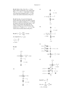
  • 1. SEDRA-ISM: “E-CH04” — 2014/11/12 — 11:02 — PAGE 1 — #1 Exercise 4–1 Ex: 4.1 Refer to Fig. 4.3(a). For vI ≥ 0, the diode conducts and presents a zero voltage drop. Thus vO = vI . For vI < 0, the diode is cut off, zero current flows through R, and vO = 0. The result is the transfer characteristic in Fig. E4.1. Ex: 4.2 See Fig. 4.3a and 4.3b. During the positive half of the sinusoid, the diode is forward biased, so it conducts resulting in vD = 0. During the negative half cycle of the input signal vI , the diode is reverse biased. The diode does not conduct, resulting in no current flowing in the circuit. So vO = 0 and vD = vI − vO = vI . This results in the waveform shown in Fig. E4.2. Ex: 4.3 ˆiD = ˆvI R = 10 V 1 k = 10 mA dc component of vO = 1 π ˆvO = 1 π ˆvI = 10 π = 3.18 V Ex: 4.4 (a) ϩ5 V V ϭ 0 V ϭ 2 mAI ϭ2.5 k⍀ 5 Ϫ 0 2.5 ϩ Ϫ (b) ϩ5 V V ϭ 5 V I ϭ 0 A2.5 k⍀ ϩ Ϫ (c) Ϫ5 V V ϭ 5 V I ϭ 0 A ϩ Ϫ 2.5 k⍀ (d) Ϫ5 V V ϭ 0 V 0 ϩ 5 2.5 I ϭ ϩ Ϫ 2.5 k⍀ϭ 2 mA (e) V ϭ 3 V 3 V 2 V 1 V 3 1 I ϭ1 k⍀ ϭ 3 mA 0 0 I (f) ϩ3 V ϩ2 V ϩ1 V I ϭ1 k⍀ ϩ5 V 0 0 I V ϭ 1 V ϭ 4 mA 5 Ϫ 1 1 ϩ Ϫ Ex: 4.5 Vavg = 10 π 50 + R = 10 π 1 mA = 10 π k ∴ R = 3.133 k
  • 2. SEDRA-ISM: “E-CH04” — 2014/11/12 — 11:02 — PAGE 2 — #2 Exercise 4–2 Ex: 4.6 Equation (4.5) V2 − V1 = 2.3 VT log I2 I1 At room temperature VT = 25 mV V2 − V1 = 2.3 × 25 × 10−3 × log 10 0.1 = 115 mV Ex: 4.7 i = IS ev/VT (1) 1 (mA) = IS e0.7/VT (2) Dividing (1) by (2), we obtain i (mA) = e(v−0.7)/VT ⇒ v = 0.7 + 0.025 ln(i) where i is in mA. Thus, for i = 0.1 mA, v = 0.7 + 0.025 ln(0.1) = 0.64 V and for i = 10 mA, v = 0.7 + 0.025 ln(10) = 0.76 V Ex: 4.8 T = 125 − 25 = 100◦ C IS = 10−14 × 1.15 T = 1.17 × 10⁻⁸ A Ex: 4.9 At 20◦ C I = 1 V 1 M = 1 μA Since the reverse leakage current doubles for every 10◦ C increase, at 40◦ C I = 4 × 1 μA = 4 μA ⇒ V = 4 μA × 1 M = 4.0 V @ 0◦ C I = 1 4 μA ⇒ V = 1 4 × 1 = 0.25 V Ex: 4.10 a. Use iteration: Diode has 0.7 V drop at 1 mA current. Assume VD = 0.7 V ID = 5 − 0.7 10 k = 0.43 mA Use Eq. (4.5) and note that V1 = 0.7 V, I1 = 1 mA ID VCC ϭ 5 V VD R ϭ 10 k⍀ ϩ Ϫ V2 − V1 = 2.3 × VT log I2 I1 V2 = V1 + 2.3 × VT log I2 I1 First iteration V2 = 0.7 + 2.3 × 25 × 10−3 log 0.43 1 = 0.679 V Second iteration I2 = 5 − 0.679 10 k = 0.432 mA V2 = 0.7 + 2.3 × 25.3 × 10−3 log 0.432 1 = 0.679 V 0.68 V we get almost the same voltage. ∴ The iteration yields ID = 0.43 mA, VD = 0.68 V b. Use constant voltage drop model: VD = 0.7 V constant voltage drop ID = 5 − 0.7 10 k = 0.43 mA Ex: 4.11 RI 10 V 2.4 V ϩ Ϫ Diodes have 0.7 V drop at 1 mA ∴ 1 mA = IS e0.7/VT (1) At a current I(mA), I = IS eVD/VT (2) Using (1) and (2), we obtain I = e(VD−0.7)/VT
  • 3. SEDRA-ISM: “E-CH04” — 2014/11/12 — 11:02 — PAGE 3 — #3 Exercise 4–3 For an output voltage of 2.4 V, the voltage drop across each diode = 2.4 3 = 0.8 V Now I, the current through each diode, is I = e(0.8−0.7)/0.025 = 54.6 mA R = 10 − 2.4 54.6 × 10−3 = 139 Ex: 4.12 (a) ϩ5 V V ϭ 0.7 V I ϭ ϭ 1.72 mA2.5 k⍀ 5 Ϫ 0.7 2.5 ϩ Ϫ (b) ϩ5 V V ϭ 5 V I ϭ 0 A 2.5 k⍀ ϩ Ϫ (c) Ϫ5 V V ϭ 5 V I ϭ 0 A ϩ Ϫ 2.5 k⍀ (d) Ϫ5 V Ϫ0.7 ϩ 5 2.5 I ϭ ϩ Ϫ 2.5 k⍀ ϭ 1.72 mA V ϭ 0.7 V (e) V ϭ 3 Ϫ 0.7 3 V 2 V 1 V 2.3 1 I ϭ I 0 0 1 k⍀ ϭ 2.3 mA ϭ 2.3 V (f) ϩ3 V 0 ϩ2 V ϩ1 V I ϭ 1 k⍀ 5 V 0 I V ϭ 1 ϩ 0.7 ϭ 1.7 V ϭ 3.3 mA 5 Ϫ 1.7 1 Ex: 4.13 rd = VT ID ID = 0.1 mA rd = 25 × 10−3 0.1 × 10−3 = 250 ID = 1 mA rd = 25 × 10−3 1 × 10−3 = 25 ID = 10 mA rd = 25 × 10−3 10 × 10−3 = 2.5 Ex: 4.14 For small signal model, iD = vD/rd (1) where rd = VT ID For exponential model, iD = IS eV/VT
  • 4. SEDRA-ISM: “E-CH04” — 2014/11/12 — 11:02 — PAGE 4 — #4 Exercise 4–4 iD2 iD1 = e(V2−V1) /VT = e vD/VT iD = iD2 − iD1 = iD1e vD /VT − iD1 = iD1 e vD/VT − 1 (2) In this problem, iD1 = ID = 1 mA. Using Eqs. (1) and (2) with VT = 25 mV, we obtain vD (mV) iD (mA) iD (mA) small exponential signal model a − 10 − 0.4 − 0.33 b − 5 − 0.2 − 0.18 c + 5 + 0.2 + 0.22 d + 10 + 0.4 + 0.49 Ex: 4.15 R IL VO ϩ15 V a. In this problem, VO iL = 20 mV 1 mA = 20 . ∴ Total small-signal resistance of the four diodes = 20 ∴ For each diode, rd = 20 4 = 5 . But rd = VT ID ⇒ 5 = 25 mV ID . ∴ ID = 5 mA and R = 15 − 3 5 mA = 2.4 k . b. For VO = 3 V, voltage drop across each diode = 3 4 = 0.75 V iD = IS eV/VT IS = iD eV/VT = 5 × 10⁻³ e0.75/0.025 = 4.7 × 10⁻¹⁶ A c. If iD = 5 − i L = 5 − 1 = 4 mA. Across each diode the voltage drop is VD = VT ln ID IS = 25 × 10−3 × ln 4 × 10⁻³ 4.7 × 10−16 = 0.7443 V Voltage drop across 4 diodes = 4 × 0.7443 = 2.977 V so change in VO = 3 − 2.977 = 23 mV. Ex: 4.16 For a zener diode VZ = VZ0 + IZ rZ 10 = VZ0 + 0.01 × 50 VZ0 = 9.5 V For IZ = 5 mA, VZ = 9.5 + 0.005 × 50 = 9.75 V For IZ = 20 mA, VZ = 9.5 + 0.02 × 50 = 10.5 V Ex: 4.17 IR 15 V 5.6 V 0 to 15 mA The minimum zener current should be 5 × IZk = 5 × 1 = 5 mA Since the load current can be as large as 15 mA, we should select R so that with IL = 15 mA, a zener current of 5 mA is available. Thus the current should be 20 mA, leading to R = 15 − 5.6 20 mA = 470 Maximum power dissipated in the diode occurs when IL = 0 is Pmax = 20 × 10−3 × 5.6 = 112 mV
  • 5. SEDRA-ISM: “E-CH04” — 2014/11/12 — 11:02 — PAGE 5 — #5 Exercise 4–5 Ex: 4.18 15 V 200 ⍀ Thus, at no load VZ 5.1 V ϩ Ϫ VZ 15 Ϫ 5.1 0.2 k⍀ I ϭ ϭ 49.5 mA 50 mA For line regulation: 200 ⍀ 7 ⍀vi vo Ϫϩ Line regulation = vo vi = 7 200 + 7 = 33.8 mV V For load regulation: 200 ⍀ VZ0 VO rZ ⌬IL VO IL = − IL(rZ 200 ) IL mA = −6.8 mV mA Ex: 4.19 ␲ vS VD 2␲ ␻t Vs ϭ 12 2 0 uu a. The diode starts conduction at vS = VD = 0.7 V vS = Vs sin ωt, here Vs = 12 √ 2 At ωt = θ, vS = Vs sin θ = VD = 0.7 V 12 √ 2 sin θ = 0.7 θ = sin−1 0.7 12 √ 2 2.4◦ Conduction starts at θ and stops at 180 − θ. ∴ Total conduction angle = 180 − 2θ = 175.2◦ b. vO,avg = 1 2π (π−θ) θ (Vs sin φ − VD) dφ = 1 2π [−Vs cos φ − VDφ]φ=π−θ φ−θ = 1 2π [Vs cos θ − Vs cos (π − θ) − VD (π − 2θ)] But cos θ 1, cos (π − θ) − 1, and π − 2θ π vO,avg = 2Vs 2π − VD 2 = Vs π − VD 2 For Vs = 12 √ 2 and VD = 0.7 V vO,avg = 12 √ 2 π − 0.7 2 = 5.05 V c. The peak diode current occurs at the peak diode voltage. ∴ ˆiD = Vs − VD R = 12 √ 2 − 0.7 100 = 163 mA PIV = +VS = 12 √ 2 17 V Ex: 4.20 ( ) ␪ ␪␲ vS Vs ϪVS Ϫ ␪␲ ϩVD output 0 input ␻t a. As shown in the diagram, the output is zero between (π − θ) to (π + θ) = 2θ
  • 6. SEDRA-ISM: “E-CH04” — 2014/11/12 — 11:02 — PAGE 6 — #6 Exercise 4–6 Here θ is the angle at which the input signal reaches VD. ∴ Vs sin θ = VD θ = sin−1 VD Vs 2θ = 2 sin−1 VD Vs b. Average value of the output signal is given by VO = 1 2π ⎡ ⎣2 × (π−θ) θ (Vs sin φ − VD) dφ ⎤ ⎦ = 1 π [−Vs cos φ − VDφ]π−θ φ=θ 2 Vs π − VD, for θ small. c. Peak current occurs when φ = π 2 . Peak current = Vs sin (π /2) − VD R = Vs − VD R If vS is 12 V(rms), then Vs = √ 2 × 12 = 12 √ 2 Peak current = 12 √ 2 − 0.7 100 163 mA Nonzero output occurs for angle = 2 (π − 2θ) The fraction of the cycle for which vO > 0 is = 2 (π − 2θ) 2π × 100 = 2 π − 2 sin−1 0.7 12 √ 2 2π × 100 97.4 % Average output voltage VO is VO = 2 Vs π − VD = 2 × 12 √ 2 π − 0.7 = 10.1 V Peak diode current ˆiD is ˆiD = Vs − VD R = 12 √ 2 − 0.7 100 = 163 mA PIV = Vs − VD + VS = 12 √ 2 − 0.7 + 12 √ 2 = 33.2 V Ex: 4.21 Vs ϪVs ϭ sin–1 ΂ ΃ 2VD output 0 2VD VS input ␪ t (a) VO,avg = 1 2π (Vs sin φ − 2VD) dφ = 2 2π [−Vs cos φ − 2VDφ]π−θ φ=θ = 1 π [Vs cos φ − Vs cos(π − θ) − 2VD(π − 2θ)] But cos θ ≈ 1, cos (π − θ) ≈ − 1 π − 2θ ≈ π. Thus ⇒ VO,avg 2Vs π − 2VD = 2 × 12 √ 2 π − 1.4 = 9.4 V (b) Peak diode current = Peak voltage R = Vs − 2VD R = 12 √ 2 − 1.4 100 = 156 mA PIV = Vs − VD = 12 √ 2 − 0.7 = 16.3 V Ex: 4.22 Full-wave peak rectifier: R C ϩ Ϫ vO vS ϩ Ϫ vS D1 D2 Vp Vr assume ideal diodes t ⌬t { T 2 The ripple voltage is the amount of voltage reduction during capacitor discharge that occurs
  • 7. SEDRA-ISM: “E-CH04” — 2014/11/12 — 11:02 — PAGE 7 — #7 Exercise 4–7 when the diodes are not conducting. The output voltage is given by vO = Vpe−t/RC Vp − Vr = Vpe− T/2 RC ← discharge is only half the period. We also assumed t T 2 . Vr = Vp 1 − e− T/2 RC e− T/2 RC 1 − T/2 RC , for CR T/2 Thus Vr Vp 1 − 1 + T/2 RC Vr = Vp 2fRC (a) Q.E.D. To find the average diode current, note that the charge supplied to C during conduction is equal to the charge lost during discharge. QSUPPLIED = QLOST iCav t = CVr SUB (a) iD,av − IL t = C Vp 2fRC = Vp 2fR = Vpπ ωR iD,av = Vpπ ω tR + IL where ω t is the conduction angle. Note that the conduction angle has the same expression as for the half-wave rectifier and is given by Eq. (4.30), ω t ∼= 2Vr Vp (b) Substituting for ω t, we get ⇒ iD,av = πVp 2Vr Vp · R + IL Since the output is approximately held at Vp, Vp R ≈ IL · Thus ⇒ iD,av ∼= πIL Vp 2Vr + IL = IL 1 + π Vp 2Vr Q.E.D. If t = 0 is at the peak, the maximum diode current occurs at the onset of conduction or at t = −ω t. During conduction, the diode current is given by iD = iC + iL iD,max = C dvS dt t=−ω t + iL assuming iL is const. iL Vp R = IL = C d dt Vp cos ωt + IL = −C sin ω t × ωVp + IL = −C sin(−ω t) × ωVp + IL For a small conduction angle sin(−ω t) ≈ − ω t. Thus ⇒ iD,max = Cω t × ωVp + IL Sub (b) to get iD,max = C 2Vr Vp ωVp + IL Substituting ω = 2πf and using (a) together with Vp/R IL results in iDmax = IL 1 + 2π Vp 2Vr Q.E.D. Ex: 4.23 ϩ ϩϪ Ϫ vS vO D2 D1 D3 D4 C R ac line voltage The output voltage, vO, can be expressed as vO = Vp − 2VD e−t/RC At the end of the discharge interval vO = Vp − 2VD − Vr The discharge occurs almost over half of the time period T/2. For time constant RC T 2
  • 8. SEDRA-ISM: “E-CH04” — 2014/11/12 — 11:02 — PAGE 8 — #8 Exercise 4–8 e−t/RC 1 − T 2 × 1 RC ∴ VP − 2VD − Vr = Vp − 2VD 1 − T 2 × 1 RC ⇒ Vr = Vp − 2VD × T 2RC Here Vp = 12 √ 2 and Vr = 1 V VD = 0.8 V T = 1 f = 1 60 s 1 = (12 √ 2 − 2 × 0.8) × 1 2 × 60 × 100 × C C = (12 √ 2 − 1.6) 2 × 60 × 100 = 1281 μF Without considering the ripple voltage, the dc output voltage = 12 √ 2 − 2 × 0.8 = 15.4 V If ripple voltage is included, the output voltage is = 12 √ 2 − 2 × 0.8 − Vr 2 = 14.9 V IL = 14.9 100 0.15 A The conduction angle ω t can be obtained using Eq. (4.30) but substituting Vp = 12 √ 2 − 2 × 0.8: ω t = 2Vr Vp = 2 × 1 12 √ 2 − 2 × 0.8 = 0.36 rad = 20.7◦ The average and peak diode currents can be calculated using Eqs. (4.34) and (4.35): iDav = IL 1 + π Vp 2Vr , where IL = 14.9 V 100 , Vp = 12 √ 2 − 2 × 0.8, and Vr = 1 V; thus iDav = 1.45 A iDmax = I 1 + 2π Vp 2Vr = 2.76 A PIV of the diodes = VS − VDO = 12 √ 2 − 0.8 = 16.2 V To provide a safety margin, select a diode capable of a peak current of 3.5 to 4A and having a PIV rating of 20 V. Ex: 4.24 Ϫ ϩ vA iD vI iϪ iϩ ϩ vD Ϫ vO 1 k⍀iR The diode has 0.7 V drop at 1 mA current. iD = IS evD/VT iD 1 mA = e(vD−0.7)/VT ⇒ vD = VT ln iD 1 mA + 0.7 V For vI = 10 mV, vO = vI = 10 mV It is an ideal op amp, so i+ = i− = 0. ∴ iD = iR = 10 mV 1 k = 10 μA vD = 25 × 10−3 ln 10 μA 1 mA + 0.7 = 0.58 V vA = vD + 10 mV = 0.58 + 0.01 = 0.59 V For vI = 1 V vO = vI = 1 V iD = vO 1 k = 1 1 k = 1 mA vD = 0.7 V VA = 0.7 V + 1 k × 1 mA = 1.7 V For vI = −1 V, the diode is cut off. ∴ vO = 0 V vA = −12 V Ex: 4.25 ϩ Ϫ vO R IL vI
  • 9. SEDRA-ISM: “E-CH04” — 2014/11/12 — 11:02 — PAGE 9 — #9 Exercise 4–9 vI > 0 ∼ diode is cut off, loop is open, and the opamp is saturated: vO = 0 V vI < 0 ∼ diode conducts and closes the negative feedback loop: vO = vI Ex: 4.26 vI vO 10 k⍀ 10 k⍀ 10 k⍀ ϩ Ϫ ϩ Ϫ Ϫ ϩ Ϫ ϩ 5 V5 V D1 D2 Both diodes are cut off for −5V ≤ vI ≤ + 5V and vO = vI For vI ≤ −5 V, diode D1 conducts and vO = −5 + 1 2 (+vI + 5) = −2.5 + vI 2 V For vI ≥ 5 V, diode D2 conducts and vO = +5 + 1 2 (vI − 5) = 2.5 + vI 2 V Ex: 4.27 Reversing the diode results in the peak output voltage being clamped at 0 V: t vO Ϫ10 V Here the dc component of vO = VO = −5 V
  • 10. SEDRA-ISM: “P-CH04-001-013” — 2014/11/12 — 15:18 — PAGE 1 — #1 Chapter 4–1 4.1 I Ϫ ϩ VD1.5 V 1 ⍀ (a) (b) I ϩ Ϫ VD1.5 V 1 ⍀ (a) The diode is reverse biased, thus I = 0 A VD = −1.5 V (b) The diode is forward biased, thus VD = 0 V I = 1.5 V 1 = 1.5 A 4.2 Refer to Fig. P4.2. (a) Diode is conducting, thus V = −3 V I = +3 − (−3) 10 k = 0.6 mA (b) Diode is reverse biased, thus I = 0 V = +3 V (c) Diode is conducting, thus V = +3 V I = +3 − (−3) 10 k = 0.6 mA (d) Diode is reverse biased, thus I = 0 V = −3 V 4.3 (a) 2 k⍀ 2 k⍀ I ϭ Cutoff Conducting D1 D2 Ϫ3 V ϩ1 V ϩ2 V V ϭ 2 V ϭ 2.5 mA 2 Ϫ(Ϫ3) (b) 2 k⍀ 2 Cutoff Conducting D1 D2 ϩ3 V ϩ1 V ϩ2 V V ϭ 1 V ϭ 1 mA 3 Ϫ(ϩ1) I ϭ 4.4 (a) 5 V 0 t vO Vp+ = 5 V Vp− = 0 V f = 1 kHz (b) Ϫ5 V 0 t vO Vp+ = 0 V Vp− = −5 V f = 1 kHz
  • 11. SEDRA-ISM: “P-CH04-001-013” — 2014/11/12 — 15:18 — PAGE 2 — #2 Chapter 4–2 (c) t0 vO vO = 0 V Neither D1 nor D2 conducts, so there is no output. (d) 5 V t vO Vp+ = 5 V, Vp− = 0 V, f = 1 kHz Both D1 and D2 conduct when vI > 0 (e) 5 V Ϫ5 V t vO Vp+ = 5 V, Vp− = −5 V, f = 1 kHz D1 conducts when vI > 0 and D2 conducts when vI < 0. Thus the output follows the input. (f) 5 V t vO Vp+ = 5 V, Vp− = 0 V, f = 1 kHz D1 is cut off when vI < 0 (g) Ϫ5 V t vO Vp+ = 0 V, Vp− = −5 V, f = 1 kHz D1 shorts to ground when vI > 0 and is cut off when vI < 0 whereby the output follows vI . (h) t vO ϭ 0 V vO = 0 V ∼ The output is always shorted to ground as D1 conducts when vI > 0 and D2 conducts when vI < 0. (i) 5 V t vO Ϫ2.5 V Vp+ = 5 V, Vp− = −2.5 V, f = 1 kHz When vI > 0, D1 is cut off and vO follows vI . When vI < 0, D1 is conducting and the circuit becomes a voltage divider where the negative peak is 1 k 1 k + 1 k × −5 V = −2.5 V (j) Ϫ2.5 V 5 V t vO Vp+ = 5 V, Vp− = −2.5 V, f = 1 kHz When vI > 0, the output follows the input as D1 is conducting. When vI < 0, D1 is cut off and the circuit becomes a voltage divider. (k) 5 V Ϫ5 V 1 V t vO Ϫ4 V Vp+ = 1 V, Vp− = −4 V, f = 1 kH3 When vI > 0, D1 is cut off and D2 is conducting. The output becomes 1 V. When vI < 0, D1 is conducting and D2 is cut off. The output becomes: vO = vI + 1 V
  • 12. SEDRA-ISM: “P-CH04-001-013” — 2014/11/12 — 15:18 — PAGE 3 — #3 Chapter 4–3 4.5 From Fig. P4.5 we see that when vI < VB; that is, vI < 3 V, D1 will be conducting the current I and iB will be zero. When vI exceeds the battery voltage (3 V), D1 cuts off and D2 conducts, thus steering I into the battery. Thus, iB will have the waveform shown in the figure. Its peak value will be 60 mA. To obtain the average value, we first determine the conduction angle of D2, (π − 2θ), where θ = sin−1 3 6 = 30◦ Thus π − 2θ = 180◦ − 60 = 120◦ The average value of iB will be iB|av = 60 × 120◦ 360◦ = 20 mA If the peak value of vI is reduced by 10%, i.e. from 6 V to 5.4 V, the peak value of iB does not change. The conduction angle of D2, however, changes since θ now becomes θ = sin−1 3 5.4 = 33.75◦ and thus π − 2θ = 112.5◦ Thus the average value of iB becomes iB|av = 60 × 112.5◦ 360◦ = 18.75 mA 4.6 A B X Y 0 0 0 0 0 1 0 1 1 0 0 1 1 1 1 1 X = AB, Y = A + B X and Y are the same for A = B X and Y are opposite if A = B 4.7 The case for the highest current in a single diode is when only one input is high: VY = 5 V VY R ≤ 0.2 mA ⇒ R ≥ 25 k 4.8 The maximum input current occurs when one input is low and the other two are high. 5 − 0 R ≤ 0.2 mA R ≥ 25 k 4.9 (a) ϩ3 V Ϫ3 V 12 k⍀ 0.33 mA 0.33 mA I ϭ 0 D2 ON D1 OFF Ϫ1 V V ϭ Ϫ1 V 6 k⍀ (a) If we assume that both D1 and D2 are conducting, then V = 0 V and the current in D2 will be [0 − (−3)]/6 = 0.5 mA. The current in the 12 k will be (3 − 0)/12 = 0.25 mA. A node equation at the common anodes node yields a negative current in D1. It follows that our assumption is wrong and D1 must be off. Now making the assumption that D1 is off and D2 is on, we obtain the results shown in Fig. (a): I = 0 V = −1 V
  • 13. SEDRA-ISM: “P-CH04-001-013” — 2014/11/12 — 15:18 — PAGE 4 — #4 Chapter 4–4 (b) ϩ3 V Ϫ3 V 6 k⍀ 3 – 0 6 0.25 mA 0 V D2 D1 ON ON ϭ 0.5 mA V ϭ 0 12 k⍀ 0 – (–3) 12 ϭ0.25 mA (b) In (b), the two resistors are interchanged. With some reasoning, we can see that the current supplied through the 6-k resistor will exceed that drawn through the 12-k resistor, leaving sufficient current to keep D1 conducting. Assuming that D1 and D2 are both conducting gives the results shown in Fig. (b): I = 0.25 mA V = 0 V 4.10 The analysis is shown on the circuit diagrams below. 4.11 R ≥ 120 √ 2 40 ≥ 4.2 k The largest reverse voltage appearing across the diode is equal to the peak input voltage: 120 √ 2 = 169.7 V These figures belong to Problem 4.10. V ϭ 2.5 V I 10 ʈ 10 ϭ 5 k⍀ 20 k⍀ (a) 10 10 ϩ 10 2.5 5 ϩ 20 5 ϫ V ϭ 0.1 ϫ 20 ϭ 2 V I ϭ ϭ 0.1 mA (b) I ϭ 0 V 2.5 V 1.5 V 5 k⍀ reverse biased 5 k⍀ V ϭ 1.5 Ϫ 2.5 ϭ Ϫ1 V Ϫ ϩ 4.12 R R ϩ RS 1 2 ϩ Ϫ vO vI vI RS D ϭ R ϩ RS vI iD ϭ ϭvI Ϫϩ D starts to conduct when vI > 0 vO vI 0 4.13 For vI > 0 V: D is on, vO = vI , iD = vI /R For vI < 0 V: D is off , vO = 0, iD = 0
  • 14. SEDRA-ISM: “P-CH04-014-030” — 2014/11/12 — 15:20 — PAGE 5 — #1 Chapter 4–5 4.14 4.15 conduction occurs R D vI vI A 12 V 0 2 ␾ ␪ ϪϪ Ϫ Ϫ Ϫ ϩ Ϫ␪ 12 V vI = A sin θ = 12 ∼ conduction through D occurs For a conduction angle (π − 2θ) that is 25% of a cycle π − 2θ 2π = 1 4 θ = π 4 A = 12/sin θ = 17 V ∴ Peak-to-peak sine wave voltage = 2A = 34 V Given the average diode current to be 1 2π 2π 0 A sin φ − 12 R dφ = 100 mA 1 2π −17 cos φ − 12φ R φ = 0.75π φ = 0.25π = 0.1 R = 8.3 Peak diode current = A − 12 R = 0.6 A Peak reverse voltage = A + 12 = 29 V For resistors specified to only one significant digit and peak-to-peak voltage to the nearest volt, choose A = 17 so the peak-to-peak sine wave voltage = 34 V and R = 8 . Conduction starts at vI = A sin θ = 12 17 sin θ = 12 θ = π 4 rad Conduction stops at π − θ. ∴ Fraction of cycle that current flows is π − 2θ 2π × 100 = 25% Average diode current = 1 2π −17 cos φ − 12φ 8 φ = 3π/4 φ = π/4 = 103 mA Peak diode current = 17 − 12 8 = 0.625 A Peak reverse voltage = A + 12 = 29 V 4.16 V RED GREEN 3 V ON OFF - D1 conducts 0 OFF OFF - No current flows –3 V OFF ON - D2 conducts 4.17 VT = kT q where k = 1.38 × 10⁻²³ J/K = 8.62 × 10⁻⁵ eV/K T = 273 + x◦ C q = 1.60 × 10⁻¹⁹ C
  • 15. SEDRA-ISM: “P-CH04-014-030” — 2014/11/12 — 15:20 — PAGE 6 — #2 Chapter 4–6 Thus VT = 8.62 × 10−5 × (273 × x◦ C), V x [◦ C] VT [mV] −55 18.8 0 23.5 +55 28.3 +125 34.3 for VT = 25 mV at 17◦ C 4.18 i = IS ev/0.025 ∴ 10,000IS = IS ev/0.025 v = 0.230 V At v = 0.7 V, i = IS e0.7/0.025 = 1.45 × 10¹² IS 4.19 I1 = IS e0.7/VT = 10−3 i2 = IS e0.5/VT i2 i1 = i2 10−3 = e 0.5 − 0.7 0.025 i2 = 0.335 μA 4.20 I = IS eVD/VT 10−3 = IS e0.7/VT (1) For VD = 0.71 V, I = IS e0.71/VT (2) Combining (1) and (2) gives I = 10−3 e(0.71 − 0.7)/0.025 = 1.49 mA For VD = 0.8 V, I = IS e0.8/VT (3) Combining (1) and (3) gives I = 10−3 × e(0.8 − 0.7)/0.025 = 54.6 mA Similarly, for VD = 0.69 V we obtain I = 10−3 × e(0.69 − 0.7)/0.025 = 0.67 mA and for VD = 0.6 V we have I = 10−3 e(0.6 − 0.7)/0.025 = 18.3 μA To increase the current by a factor of 10, VD must be increased by VD, 10 = e VD/0.025 ⇒ VD = 0.025 ln10 = 57.6 mV 4.21 IS can be found by using IS = ID · e−VD/VT . Let a decrease by a factor of 10 in ID result in a decrease of VD by V: ID = IS eVD/VT ID 10 = IS e(VD− V)/VT = IS eVD/VT · e− V/VT Taking the ratio of the above two equations, we have 10 = e V/VT ⇒ V 60 mV Thus the result in each case is a decrease in the diode voltage by 60 mV. (a) VD = 0.700 V, ID = 1 A ⇒ IS = 6.91 × 10⁻¹³ A; 10% of ID gives VD = 0.64 V (b) VD = 0.650 V, ID = 1 mA ⇒ IS = 5.11 × 10⁻¹⁵ A; 10% of ID gives VD = 0.59 V (c) VD = 0.650 V, ID = 10 μA ⇒ IS = 5.11 × 10⁻¹⁷ A; 10% of ID gives VD = 0.59 V (d) VD = 0.700 V, ID = 100 mA ⇒ IS = 6.91 × 10⁻¹⁴ A; 10% of ID gives VD = 0.64 V 4.22 IS can be found by using IS = ID · e−VD/VT . Let an increase by a factor of 10 in ID result in an increase of VD by V: ID = IS eVD/VT 10ID = IS e(VD+ V)/VT = IS eVD/VT · e V/VT Taking the ratio of the above two equations, we have 10 = e V/VT ⇒ V 60 mV Thus the result is an increase in the diode voltage by 60 mV. Similarly, at ID/10, VD is reduced by 60 mV.
  • 16. SEDRA-ISM: “P-CH04-014-030” — 2014/11/12 — 15:20 — PAGE 7 — #3 Chapter 4–7 (a) VD = 0.70 V, ID = 10 mA ⇒ IS = 6.91 × 10⁻¹⁵ A; ID × 10 gives VD = 0.76 V ID/10 gives VD = 0.64 V (b) VD = 0.70 V, ID = 1 mA ⇒ IS = 6.91 × 10⁻¹⁶ A; ID × 10 gives VD = 0.76 V ID/10 gives VD = 0.64 V (c) VD = 0.80 V, ID = 10 A ⇒ IS = 1.27 × 10⁻¹³ A; ID × 10 gives VD = 0.86 V ID/10 gives VD = 0.74 V (d) VD = 0.70 V, ID = 1 mA ⇒ IS = 6.91 × 10⁻¹⁶ A; ID × 10 gives VD = 0.76 V ID/10 gives VD = 0.64 V (e) VD = 0.6 V, ID = 10 μA ⇒ IS = 3.78 × 10⁻¹⁶ A ID × 10 gives VD = 0.66 V ID/10 gives VD = 0.54 V 4.23 The voltage across three diodes in series is 2.0 V; thus the voltage across each diode must be 0.667 V. Using ID = IS eVD/VT , the required current I is found to be 3.9 mA. If 1 mA is drawn away from the circuit, ID will be 2.9 mA, which would give VD = 0.794 V, giving an output voltage of 1.98 V. The change in output voltage is −22 mV. 4.24 Connecting an identical diode in parallel would reduce the current in each diode by a factor of 2. Writing expressions for the currents, we have ID = IS eVD/VT ID 2 = IS e(VD− V)/VT = IS eVD/VT · e− V/VT Taking the ratio of the above two equations, we have 2 = e V/VT ⇒ V = 17.3 mV Thus the result is a decrease in the diode voltage by 17.3 mV. 4.25 VD ϩ Ϫ I ID2 ID1 D1 D2 ID1 = IS1eVD/VT (1) ID2 = IS2eVD/VT (2) Summing (1) and (2) gives ID1 + ID2 = (IS1 + IS2)eVD/VT But ID1 + ID2 = I Thus I = (IS1 + IS2) eVD/VT (3) From Eq. (3) we obtain VD = VT ln I IS1 + IS2 Also, Eq. (3) can be written as I = IS1 eVD/VT 1 + IS2 IS1 (4) Now using (1) and (4) gives ID1 = I 1 + (IS2/IS1) = I IS1 IS1 + IS2 We similarly obtain ID2 = I 1 + (IS1/IS2) = I IS2 IS1 + IS2 4.26 I D2 D3 8I1 D4 4I12I1 I1 ϭ 0.1 mA I1 D1
  • 17. SEDRA-ISM: “P-CH04-014-030” — 2014/11/12 — 15:20 — PAGE 8 — #4 Chapter 4–8 The junction areas of the four diodes must be related by the same ratios as their currents, thus A4 = 2A3 = 4A2 = 8 A1 With I1 = 0.1 mA, I = 0.1 + 0.2 + 0.4 + 0.8 = 1.5 mA 4.27 We can write a node equation at the anodes: ID2 = I1 − I2 = 7 mA ID1 = I2 = 3 mA We can write the following equation for the diode voltages: V = VD2 − VD1 If D2 has saturation current IS , then D1, which is 10 times larger, has saturation current 10IS . Thus we can write ID2 = IS eVD2/VT ID1 = 10IS eVD1/VT Taking the ratio of the two equations above, we have ID2 ID1 = 7 3 = 1 10 e(VD2−VD1)/VT = 1 10 eV/VT ⇒ V = 0.025 ln 70 3 = 78.7 mV To instead achieve V = 60 mV, we need ID2 ID1 = I1 − I2 I2 = 1 10 e0.06/0.025 = 1.1 Solving the above equation with I1 still at 10 mA, we find I2 = 4.76 mA. 4.28 We can write the following node equation at the diode anodes: ID2 = 10 mA − V/R ID1 = V/R We can write the following equation for the diode voltages: V = VD2 − VD1 We can write the following diode equations: ID2 = IS eVD2/VT ID1 = IS eVD1/VT Taking the ratio of the two equations above, we have ID2 ID1 = 10 mA − V/R V/R = e(VD2−VD1)/VT = eV/VT To achieve V = 50 mV, we need ID2 ID1 = 10 mA − 0.05/R 0.05/R = e0.05/0.025 = 7.39 Solving the above equation, we have R = 42 4.29 For a diode conducting a constant current, the diode voltage decreases by approximately 2 mV per increase of 1◦ C. T = −20◦ C corresponds to a temperature decrease of 40◦ C, which results in an increase of the diode voltage by 80 mV. Thus VD = 770 mV. T = + 85◦ C corresponds to a temperature increase of 65◦ C, which results in a decrease of the diode voltage by 130 mV. Thus VD = 560 mV. 4.30 D2 D1 R1 I ϩ10 V V1 ϩ Ϫ V2 ϩ Ϫ At 20◦ C: VR1 = V2 = 520 mV R1 = 520 k I = 520 mV 520 k = 1 μA Since the reverse current doubles for every 10◦ C rise in temperature, at 40◦ C, I = 4 μA V2 ID2 480 40°C 40 mV 20°C 520 mV 4 µA 1 µA V2 = 480 + 2.3 × 1 × 25 log 4 = 514.6 mV VR1 = 4 μA × 520 k = 2.08 V At 0◦ C, I = 1 4 μA V2 = 560 − 2.3 × 1 × 25 log 4 = 525.4 mV VR1 = 1 4 × 520 = 0.13 V
  • 18. SEDRA-ISM: “P-CH04-031-053” — 2014/11/12 — 17:25 — PAGE 9 — #1 Chapter 4–9 4.31 For a diode conducting a constant current, the diode voltage decreases by approximately 2 mV per increase of 1◦ C. A decrease in VD by 100 mV corresponds to a junction temperature increase of 50◦ C. The power dissipation is given by PD = (10 A) (0.6 V) = 6 W The thermal resistance is given by T PD = 50◦ C 6 W = 8.33◦ C/W 4.32 Given two different voltage/current measurements for a diode, we can write ID1 = IS eVD1/VT ID2 = IS eVD2/VT Taking the ratio of the above two equations, we have ID1 ID2 = IS e(VD1−VD2)/VT ⇒ VD1 − VD2 = VT ln ID1 ID2 For ID = 1 mA, we have V = VT ln 1 × 10⁻³ A 10 A = −230 mV ⇒ VD = 570 mV For ID = 3 mA, we have V = VT ln 3 × 10⁻³ A 10 A = −202 mV ⇒ VD = 598 mV Assuming VD changes by –2 mV per 1◦ C increase in temperature, we have, for ±20◦ C changes: For ID = 1 mA, 530 mV ≤ VD ≤ 610 mV For ID = 3 mA, 558 mV ≤ VD ≤ 638 mV Thus the overall range of VD is between 530 mV and 638 mV. 4.33 Given two different voltage/current measurements for a diode, we have ID1 ID2 = IS e(VD1−VD2)/VT ⇒ VD1 − VD2 = VT ln ID1 ID2 For the first diode, with ID = 0.1 mA and VD = 700 mV, we have ID = 1 mA: V = VT ln 1.0 0.1 = 57.6 mV ⇒ VD = 757.6 mV ID = 3 mA: V = VT ln 3 0.1 = 85 mV ⇒ VD = 785 mV For the second diode, with ID = 1 A and VD = 700 mV, we have ID = 1.0 mA: V = VT ln 0.001 1 = −173 mV ⇒ VD = 527 mV ID = 3 mA: V = VT ln 0.003 1 = −145 mV ⇒ VD = 555 mV For both ID = 1.0 mA and ID = 3 mA, the difference between the two diode voltages is approximately 230 mV. Since, for a fixed diode current, the diode voltage changes with temperature at a constant rate (–2 mV per ◦ C temp. increase), this voltage difference will be independent of temperature! 4.34 Ϫ ϩ VDD R ϭ 1 kΩ 1 V i v IS = 10−15 A = 10−12 mA Calculate some points v = 0.6 V, i = IS ev/VT = 10−12 e0.6/0.025 0.03 mA v = 0.65 V, i 0.2 mA v = 0.7 V, i 1.45 mA Make a sketch showing these points and load line and determine the operating point. The points for the load line are obtained using ID = VDD − VD R
  • 19. SEDRA-ISM: “P-CH04-031-053” — 2014/11/12 — 17:25 — PAGE 10 — #2 Chapter 4–10 Load line 0.4 0 0.2 0.4 0.6 0.8 1.0 2.0 i (mA) 0.6 0.8 1.0 v (V) Diode characteristic From this sketch one can see that the operating point must lie between v = 0.65 V to v = 0.7 V For i = 0.3 mA, v = VT ln i IS = 0.025 × ln 3 10−12 = 0.661 V For i = 0.4 mA, v = 0.668 V Now we can refine the diagram to obtain a better estimate i (mA) Load line 0.30 0.660 0.664 0.67 0.35 0.4 v (V) From this graph we get the operating point i = 0.338 mA, v = 0.6635 V Now we compare graphical results with the exponential model. At i = 0.338 mA v = VT ln i IS = 0.025 × ln 0.338 10−12 = 0.6637 V The difference between the exponential model and graphical results is = 0.6637 − 0.6635 = 0.0002 V = 0.2 mV 4.35 R ϭ 1 k⍀ 1 V Ϫ ϩ Ϫ ϩ VDID IS = 10−15 A = 10−12 mA Use the iterative analysis procedure: 1. VD = 0.7 V, ID = 1 − 0.7 1 K = 0.3 mA 2. VD = VT ln ID IS = 0.025 ln 0.3 10−12 || = 0.6607 V ID = 1 − 0.6607 1 K = 0.3393 mA 3. VD = 0.025 ln 0.3393 10−12 = 0.6638 V ID = 1 − 0.6638 1 K = 0.3362 mA 4. VD = 0.025 ln 0.3362 10−12 = 0.6635 V ID = 1 − 0.6635 1 k = 0.3365 mA Stop here as we are getting almost same value of ID and VD 4.36 500 ⍀ 1 V Ϫ ϩ Ϫ ϩ vi a) ID = 1 − 0.7 0.5 k = 0.6 mA b) Diode has 0.7 V drop at 1 mA current. Use Eq. (4.5): v2 = v1 + 2.3VT log i2 i1 1. v = 0.7 V 1 i = 1 − 0.7 0.5 k = 0.6 mA 2. v = 0.7 + 2.3 × 0.025 log 0.6 1 = 0.6872 V 2 i = 1 − 0.6872 0.5 = 0.6255 mA
  • 20. SEDRA-ISM: “P-CH04-031-053” — 2014/11/12 — 17:25 — PAGE 11 — #3 Chapter 4–11 3. v = 0.7 + 2.3 × 0.025 log 0.6255 1 = 0.6882 V 3 i = 1 − 0.6882 0.5 k = 0.6235 mA 4. v = 0.7 + 2.3 × 0.025 log 0.6235 1 = 0.6882 V 4 i = 1 − 0.6882 0.5 k = 0.6235 mA Stop as we are getting the same result. 4.37 We first find the value of IS for the diode, given by IS = IDe−VD/VT with ID = 1 mA and VD = 0.75 V. This gives IS = 9.36 × 10⁻¹⁷ A. In order to have 3.3 V across the 4 series-connected diodes, each diode drop must be 0.825 V. Applying this voltage to the diode gives current ID = 20.1 mA. We can then find the resistor value using R = 15 V − 3.3 V 20.1 mA = 582 4.38 Constant voltage drop model: Using vD = 0.7 V, ⇒ iD1 = V − 0.7 R Using vD = 0.6 V, ⇒ iD2 = V − 0.6 R For the difference in currents to be only 1%, ⇒ iD2 = 1.01iD1 V − 0.6 = 1.01 (V − 0.7) V = 10.7 V For V = 3 V and R = 1 k : At VD = 0.7 V, iD1 = 3 − 0.7 1 = 2.3 mA At VD = 0.6 V, iD2 = 3 − 0.6 1 = 2.4 mA iD2 iD1 = 2.4 2.3 = 1.04 Thus the percentage difference is 4%. 4.39 Available diodes have 0.7 V drop at 2 mA current since 2VD = 1.4 V is close to 1.3 V, use N parallel pairs of diodes to split the 1 mA current evenly, as shown in the figure next. N 1 mA Ϫ ϩ V The voltage drop across each pair of diodes is 1.3 V. ∴ Voltage drop across each diode = 1.3 2 = 0.65 V. Using I2 = I1e(V2−V1)/VT = 2e(0.65−0.7)/0.025 = 0.2707 mA Thus current through each branch is 0.2707 mA. The 1 mA will split in = 1 0.2707 = 3.69 branches. Choose N = 4. There are 4 pairs of diodes in parallel. ∴ We need 8 diodes. Current through each pair of diodes = 1 mA 4 = 0.25 mA ∴ Voltage across each pair = 2 0.7 + 0.025 ln 0.25 2 = 1.296 V SPECIAL NOTE: There is another possible design utilizing only 6 diodes and realizing a voltage of 1.313 V. It consists of the series connection of 4 parallel diodes and 2 parallel diodes. 4.40 Refer to Example 4.2. (a) 10 k⍀ 5 k⍀ ϩ10 V 1.86Ϫ1 ϭ 0.86 mA Ϫ10 V V ϭ 0 V I ϭ ϭ 1.86 mA ϭ1 mA ⌷⌵⌷⌵ Ϫ0.7 V Ϫ0.7 ϩ 10 5 2 10 Ϫ 0 10 3 45 1
  • 21. SEDRA-ISM: “P-CH04-031-053” — 2014/11/12 — 17:25 — PAGE 12 — #4 Chapter 4–12 (b) Cutoff 5 k⍀ 10 k⍀ ID2 ϩ10 V Ϫ10 V 0.7 V V I ϭ 0 ID2 ϩ Ϫ⌷⌵ ID2 = 10 − (−10) − 0.7 15 = 1.29 mA VD = −10 + 1.29 (10) + 0.7 = 3.6 V 4.41 (a) 10 k⍀ ϩ3 V Ϫ3 V V I V = −3 + 0.7 = −2.3 V I = 3 + 2.3 10 = 0.53 mA (b) 10 k⍀ Cutoff ϩ3 V Ϫ3 V V I I = 0 A V = 3 − I (10) = 3 V (c) 10 k⍀ ϩ3 V I Ϫ3 V V V = 3 − 0.7 = 2.3 V I = 2.3 + 3 10 = 0.53 mA (d) ϩ3 V Ϫ3 V Cutoff I V I = 0 A V = −3 V 4.42 (a) 2 k⍀ Cutoff Ϫ3 V ϩ1 V ϩ2 V I V D1 D2 V = 2 − 0.7 = 1.3 V I = 1.3 − (−3) 2 = 2.15 mA
  • 22. SEDRA-ISM: “P-CH04-031-053” — 2014/11/12 — 17:25 — PAGE 13 — #5 Chapter 4–13 (b) 2 k⍀ Cutoff ϩ3 V I Vϩ1 V D1 D2 ϩ2 V V = 1 + 0.7 = 1.7 V I = 3 − 1.7 2 = 0.65 mA 4.43 6 k⍀ + 3 V ϩ ᎐ Ϫ3 V 0.7 V 12 k⍀ V I ϭ 0 ID2 ID2 D1 D2 Cutoff (a) ON 12 k⍀ ϩ 3 V ϩ 0.7 V Ϫ3 V 6 k⍀ (b) I ϭ 0.383 ᎐ 0.25 V ϭ 0 V D1 D2 ONON 6 ϭ 0.383 mA ϭ 0.133 mA 3Ϫ0.7 12 0.25 mA 0Ϫ(Ϫ3) ϭ (a) ID2 = 3 − 0.7 − (−3) 12 + 6 = 0.294 mA V = −3 + 0.294 × 6 = −1.23 V Check that D1 is off: Voltage at the anode of D1 = V + VD2 = −1.23 + 0.7 = −0.53 V which keeps D1 off. (b) See analysis on Fig. (b). I = 0.133 mA V = 0 V 4.44 I 20 k⍀ 10 ʈ 10 ϭ 5 k⍀ 0.7 V 10 10 ϩ 10 5 ϫ (a) V ϩ ᎐ ϭ 2.5 V 1.5 V Ϫ V ϩ5 k⍀ 5 k⍀ 2.5 V 0 mA (b) (a) I = 2.5 − 0.7 5 + 20 = 0.072 mA V = 0.072 × 20 = 1.44 V (b) The diode will be cut off, thus I = 0 V = 1.5 − 2.5 = −1 V 4.45 vI iD R Ϫ ϩ iD,peak = vI,peak − 0.7 R ≤ 40 mA R ≥ 120 √ 2 − 0.7 40 = 4.23 k Reverse voltage = 120 √ 2 = 169.7 V. The design is essentially the same since the supply voltage 0.7 V 4.46 Use the exponential diode model to find the percentage change in the current. iD = IS ev/VT iD2 iD1 = e(V2−V1)/VT = e v/VT For +5 mV change we obtain
  • 23. SEDRA-ISM: “P-CH04-031-053” — 2014/11/12 — 17:25 — PAGE 14 — #6 Chapter 4–14 iD2 iD1 = e5/25 = 1.221 % change = iD2 − iD1 iD1 × 100 = 1.221 − 1 1 × 100 = 22.1% For –5 mV change we obtain iD2 iD1 = e−5/25 = 0.818 % change = iD2 − iD1 iD1 × 100 = 0.818 − 1 1 × 100 = −18.1% Maximum allowable voltage signal change when the current change is limited to ±10% is found as follows: The current varies from 0.9 to 1.1 iD2 iD1 = e V/VT For 0.9, V = 25 ln (0.9) = −2.63 mV For 1.1, V = 25 ln (1.1) = +2.38 mV For ±10% current change the voltage signal change is from –2.63 mV to +2.38 mV 4.47 0.1 A Ten diode connected in parallel and fed with a total current of 0.1 A. So the current through each diode = 0.1 10 = 0.01 A Small signal resistance of each diode = VT iD = 25 mV 0.01 A = 2.5 Equivalent resistance, Req, of 10 diodes connected in parallel is given by Req = 2.5 10 = 0.25 If there is one diode conducting 0.1 A current, then the small signal resistance of this diode = 25 mV 0.1 A = 0.25 This value is the same as of 10 diodes connected in parallel. If 0.2 is the resistance for making connection, the resistance in each branch = rd + 0.2 = 2.5 + 0.2 = 2.7 For a parallel combination of 10 diodes, equivalent resistance, Req, is Req = 2.7 10 = 0.27 If there is a single diode conducting all the 0.1 A current, the connection resistance needed for the single diode will be = 0.27 − 0.25 = 0.02 . 4.48 The dc current I flows through the diode giving rise to the diode resistance rd = VT I and the small-signal equivalent circuit is represented by vovs rd ϩ Ϫ Rs vo = vs × rd rd + RS = vs VT /I VT I + RS = vs VT VT + IRS Now, vo = 10 mV × 25 mV 25 mV + 103 I I vo 1 mA 0.24 mV 0.1 mA 2.0 mV 1 μA 9.6 mV For vo = 1 2 vs = vs × 0.025 0.025 + 103 I ⇒ I = 25 μA 4.49 As shown in Problem 4.48, vo vi = VT VT + RS I = 0.025 0.025 + 104 I (1) Here RS = 10 k The current changes are limited ±10%. Using exponential model, we get iD2 iD1 = e v/VT = 0.9 to 1.1 v = 25 × 10−3 ln iD2 iD1 and here For 0.9, v = −2.63 mV For 1.1, v = 2.38 mV The variation is –2.63 mV to 2.38 mV for ±10% current variation. Thus the largest symmetrical output signal allowed is 2.38 mV in amplitude. To
  • 24. SEDRA-ISM: “P-CH04-031-053” — 2014/11/12 — 17:25 — PAGE 15 — #7 Chapter 4–15 obtain the corresponding input signal, we divide this by (vo/vi): ˆvs = 2.38 mV vo/vi (2) Now for the given values of vo/vi calculate I and ˆvS using Equations (1) and (2) vo vi I in mA ˆvs in mV 0.5 0.0025 4.76 0.1 0.0225 23.8 0.01 0.2475 238 0.001 2.4975 2380 4.50 vo vi C2 1 mA D1 D2 I C1 When both D1 and D2 are conducting, the small-signal model is vovi rd2 rd1 where we have replaced the large capacitors C1 and C2 by short circuits: vo vi = rd2 rd1 + rd2 = VT 1 m − I VT I + VT 1 m − I = I 1 m Thus vo vi = I, where I is in mA Now I = 0 μA, vo vi = 0 I = 1 μA, vo vi = 1 × 10−3 = 0.001 V/V I = 10 μA, vo vi = 10 × 10−3 = 0.01 V/V I = 100 μA, vo vi = 100 × 10−3 = 0.1 V/V I = 500 μA, vo vi = 500 × 10−3 = 0.5 V/V I = 600 μA, vo vi = 600 × 10−3 = 0.6 V/V I = 900 μA, vo vi = 900 × 10−3 = 0.9 V/V I = 990 μA, vo vi = 990 × 10−3 = 0.99 V/V I = 1 mA = 1000 μA, vo vi = 1000 × 10−3 = 1 V/V 4.51 I D1 D3 D2 vo vi D4 I R 10 k⍀ a. The current through each diode is I 2 : rd = VT I 2 = 2VT I = 0.05 I From the equivalent circuit vo vi = R R + (2rd 2rd ) = R R + rd I rd vo vi 0 μA ∞ 0 1 μA 50 k 0.167 10 μA 5 k 0.667 100 μA 500 0.952 1 mA 50 0.995 10 mA 5 0.9995
  • 25. SEDRA-ISM: “P-CH04-031-053” — 2014/11/12 — 17:25 — PAGE 16 — #8 Chapter 4–16 Equivalent Circuit rd rd rd rdvI vo R 10 k⍀Ϫϩ b. For signal current to be limited to ±10% of I (I is the biasing current), the change in diode voltage can be obtained from the equation iD I = e VD/VT = 0.9 to 1.1 vD = −2.63 mV to +2.32 mV ±2.5 mV so the signal voltage across each diode is limited to 2.5 mV when the diode current remains within 10% of the dc bias current. ∴ vo = 10 − 2.5 − 2.5 = 5 mV and i = 5 mV 10 k = 0.5 μA vo R 10 k⍀Ϫϩ ϩ2.5Ϫ mV ϩ2.5Ϫ mV ϩ2.5Ϫ mV ϩ2.5Ϫ mV 10 mV i The current through each diode = 0.5 2 μA = 0.25 μA The signal current i is 0.5 μA, and this is 10% of the dc biasing current. ∴ DC biasing current I = 0.5 × 10 = 5 μA c. Now I = 1 mA. ∴ ID = 0.5 mA Maximum current derivation 10%. ∴ id = 0.5 10 = 0.05 mA and i = 2id = 0.1 mA. ∴ Maximum vo = i × 10 k = 0.1 × 10 = 1 V From the results of (a) above, for I = 1 mA, vo/vi = 0.995; thus the maximum input signal will be ˆvi = ˆvo/0.995 = 1/0.995 = 1.005 V The same result can be obtained from the figure above where the signal across the two series diodes is 5 mV, thus ˆvi = ˆvo + 5 mV = 1 V + 5 mV = 1.005 V. See also the figure below. 4.52 I v1 D1 i1 i3 i2 i4 D3 D2 iO vO D4 R 10 k⍀ v2 v4 v3 ϩ ϩ ϩ ϩ Ϫ Ϫ Ϫ Ϫ I vI I = 1 mA Each diode exhibits 0.7 V drop at 1 mA current. Using diode exponential model we have v2 − v1 = VT ln i2 i1 and v1 = 0.7 V, i1 = 1 mA ⇒ v = 0.7 + VT ln i 1 = 700 + 25 ln(i)
  • 26. SEDRA-ISM: “P-CH04-031-053” — 2014/11/12 — 17:25 — PAGE 17 — #9 Chapter 4–17 Calculation for different values of vO: vO = 0, iO = 0, and the current I = 1 mA divide equally between the D3, D4 side and the D1, D2 side. i1 = i2 = i3 = i4 = I 2 = 0.5 mA v = 700 + 25 ln(0.5) 683 mV v1 = v2 = v3 = v4 = 683 mV From the circuit, we have vI = −v1 + v3 + vO = −683 + 683 + 0 = 0 V For vO = 1 V, iO = 1 10 k = 0.1 mA Because of symmetry of the circuit, we obtain i3 = i2 = I 2 + iO 2 = 0.5 + 0.05 = 0.55 mA and i4 = i1 = 0.45 mA v3 = v2 = 700 + 25 ln i2 1 = 685 mV v4 = v1 = 700 + 25 ln i4 1 = 680 mV vO iO i3 = i2 i4 = i1 v3 = v2 v4 = v1 vI = −v1+ (V) (mA) (mA) (mA) (mV) (mV) v3 + vO (V) 0 0 0.5 0.5 683 683 0 + 1 0.1 0.55 0.45 685 680 1.005 + 2 0.2 0.6 0.4 ∼ 687 677 2.010 + 5 0.5 0.75 0.25 ∼ 693 665 5.028 + 9 0.9 0.95 0.05 ∼ 699 ∼ 625 9.074 + 9.9 0.99 0.995 0.005 ∼ 700 568 10.09 9.99 0.999 0.9995 0.0005 ∼ 700 510 10.18 10 1 1 0 700 0 10.7 vI = −v1 + v2 + vO = −0.680 +0.685 + 1 = 1.005 V Similarly, other values are calculated as shown in the table. The largest values of vO on positive and negative side are +10 V and −10 V, respectively. This restriction is imposed by the current I = 1 mA A similar table can be generated for the negative values. It is symmetrical. For vI > +10.7, vO will be saturated at +10 V and it is because I = 1 mA. Similarly, for vI < −10.7 V, vO will be saturated at −10 V. For I = 0.5 mA, the output will saturate at 0.5 mA ×10 k = 5 V. vo (V) v1 (V) 10 5 Ϫ5 Ϫ5.68 5.68Ϫ10.7 10.7 I ϭ 1 mA I ϭ 0.5 mA 4.53 Representing the diode by the small-signal resistances, the circuit is vi VT vo ID C ϩ Ϫ Ϫϭ rd rd Ϫϩ Vo Vi = 1 sC rd + 1 sC = 1 1 + sCrd Vo Vi = 1 1 + jωCrd Phase shift = −tan−1 ωCrd 1 = −tan−1 ωC VT I For phase shift of −45◦ , we obtain −45 = −tan−1 2π × 100 × 103 × 10 × 10−9 × 0.025 I ⇒ I = 157 μA Now I varies from 157 10 μA to 157 × 10 μA Range is 15.7 μA to 1570 μA Range of phase shift is −84.3◦ to −5.71◦
  • 27. SEDRA-ISM: “P-CH04-054-069” — 2014/11/12 — 15:21 — PAGE 18 — #1 Chapter 4–18 4.54 Vϩ VO R ϩ Ϫ (a) VO V+ = rd R + rd = VT /I R + VT I = VT IR + VT For no load, I = V+ − VO R = V+ − 0.7 R . ∴ VO V+ = VT VT + (V+ − 0.7) Small-signal model ϩ Ϫ R ⌬V rd ⌬VOϪϩϩ (b) If m diodes are in series, we obtain VO V+ = mrd mrd + R = mVT mVT + IR = mVT mVT + (V+ − 0.7m) (c) For m = 1 VO V+ = VT VT + V+ − 0.7 = 1.75 mV/V For m = 4 VO V+ = mVT mVT + 15 − m × 0.7 = 8.13 mV/V 4.55 R Small-signal model ϩ Ϫ IL IL rdR ⌬VO Vϩ VO (a) From the small-signal model VO = −IL (rd R) VO IL = − (rd R) (b) At no load, ID = V+ − 0.7 R rd = VT ID VO IL = − (rd R) = − 1 1 rd + 1 R = − 1 ID V+ − 0.7 + ID VT = − VT ID × 1 VT V+ − 0.7 + 1 = − VT ID × V+ − 0.7 VT + V+ − 0.7 For VO IL ≤ 5 mV mA i.e., VT ID × V+ − 0.7 VT + V+ − 0.7 ≤ 5 mV mA 25 ID × 15 − 0.7 0.025 + 15 − 0.7 ≤ 5 mV mA ID ≥ 4.99 mA ID 5 mA R = V+ − 0.7 ID = 15 − 0.7 5 mA R = 2.86 k
  • 28. SEDRA-ISM: “P-CH04-054-069” — 2014/11/12 — 15:21 — PAGE 19 — #2 Chapter 4–19 Diode should be a 5-mA unit; that is, it conducts 5 mA at VD = 0.7 V, thus 5 × 10−3 = IS e0.7/0.025 . ⇒ IS = 3.46 × 10⁻¹⁵ A (c) For m diodes connected in series we have ID = V+ − 0.7m R and rd = VT ID So now VO IL = −(R mrd ) = − 1 1 R + 1 mrd = − 1 ID V+ − 0.7m + ID mVT = − mVT ID mVT V+ − 0.7m + 1 = − mVT ID V+ − 0.7m V+ − 0.7m + mVT 4.56 IL ID Vo I ϩ5 V RL R Diode has 0.7 V drop at 1 mA current VO = 1.5 V when RL = 1.5 k ID = IS eV/VT 1 × 10−3 = IS e0.7/0.025 ⇒ IS = 6.91 × 10⁻¹⁶ A Voltage drop across each diode = 1.5 2 = 0.75 V. ∴ ID = IS eV/VT = 6.91 × 10⁻¹⁶ × e0.75/0.025 = 7.38 mA IL = 1.5/1.5 = 1 mA I = ID + IL = 7.39 mA + 1 mA = 8.39 mA ∴ R = 5 − 1.5 8.39 mA = 417 Use a small-signal model to find voltage VO when the value of the load resistor, RL, changes: rd = VT ID = 0.025 7.39 = 3.4 When load is disconnected, all the current I flows through the diode. Thus ID = 1 mA VO = ID × 2rd = 1 × 2 × 3.4 = 6.8 mV With RL = 1 k , IL 1.5 V 1 = 1.5 mA IL = 0.5 mA ID = −0.5 mA VO = −0.5 × 2 × 3.4 = −3.4 mV With RL = 750 , IL 1.5 0.75 = 2 mA IL = 1 mA ID = −1 mA VO = −1 × 2 × 3.4 = −6.8 mV With RL = 500 , IL 1.5 0.5 = 3 mA IL = 2.0 mA ID = −2.0 mA VO = −2 × 2 × 3.4 = −13.6 mV
  • 29. SEDRA-ISM: “P-CH04-054-069” — 2014/11/12 — 15:21 — PAGE 20 — #3 Chapter 4–20 4.57 IL IL varies from 2 to 7 mA ID I ϭ 1.5 Vϩ ⌬VOvO To supply a load current of 2 to 7 mA, the current I must be greater than 7 mA. So I can be only 10 mA or 15 mA. Now let us evaluate VO for both 10-mA and 15-mA sources. For the 10-mA source: Since IL varies from 2 to 7 mA, the current ID will varry from 8 to 3 mA. Correspondingly, the voltage across each diode changes by VD where 3 8 = e VD/VT ⇒ VD = 25 ln 3 8 = −24.5 mV and the output voltage changes by VO = 2 × VD = −49 mV With I = 15 mA, the diodes current changes from 13 to 8 mA. Correspondingly, the voltage across each diode changes by VD where 8 13 = e VD/VT ⇒ VD = 25 ln 8 13 = −12.1 mV and the output voltage changes by VO = 2 × VD = −24.2 mV which is less than half that obtained with the 10-mA supply. Thus, from the point of view of reducing the change in VO as IL changes, we choose the 15-mA supply. Note, however, that the price paid is increased power dissipation. 4.58 IL ID D1 D2 I ϩ5 V ϩ ᎐ RL ϭ 150 ⍀ R ϭ 200 ⍀ VO (a) Iteration #1: VD = 0.7 V VO = 2VD = 1.4 V IL = VO RL = 1.4 0.15 = 9.33 mA I = 5 − VO R = 5 − 1.4 0.2 = 18 mA ID = I − IL = 18 − 9.33 = 8.67 mA Iteration #2: VD = 0.7 + 0.025 ln 8.67 10 = 0.696 V VO = 1.393 V IL = 9.287 mA I = 5 − 1.393 0.2 = 18.04 mA ID = 18.04 − 9.287 = 8.753 mA Iteration #3: VD = 0.7 + 0.025 ln 8.753 10 = 0.697 VO = 1.393 V IL = 9.287 I = 18.04 mA ID = 8.753 No further iterations are necessary and VO = 1.39 V (b) With no load: Iteration #1: VD = 0.7 V VO = 1.4 V
  • 30. SEDRA-ISM: “P-CH04-054-069” — 2014/11/12 — 15:21 — PAGE 21 — #4 Chapter 4–21 I = 5 − 1.4 0.2 = 18 mA ID = I = 18 mA Iteration #2: VD = 0.7 + 0.025 ln 18 10 = 0.715 V VO = 1.429 V I = 17.85 mA ID = 17.85 mA Iteration #3: VD = 0.7 + 0.025 ln 17.85 10 = 0.714 V VO = 1.43 V I = 17.86 mA ID = 17.86 mA No further iterations are warranted and VO = 1.43 V (c) VO = 1.39 − 0.1 = 1.29 V IL = 1.29 0.15 = 8.6 mA VD = 1.29 2 = 0.645 V ID = 10 × e(0.645−0.7)/0.025 = 1.11 mA I = IL + ID = 8.6 + 1.11 = 9.71 mA VSupply = VO + IR = 1.29 + 9.71 × 0.2 = 3.232 V which is a reduction of 1.768 V or −35.4%. (d) For VSupply = 5 + 1.786 = 6.786 V, Iteration #1: VD = 0.7 V VO = 1.4 V IL = 9.33 mA I = 6.768 − 1.4 0.2 = 26.84 ID = I − IL = 26.84 − 9.33 = 17.51 mA Iteration #2: VD = 0.7 + 0.025 ln 17.51 10 = 0.714 V VO = 1.428 V IL = 9.52 mA I = 26.70 mA ID = 17.18 mA Iteration #3: VD = 0.7 + 0.025 ln 17.18 10 = 0.714 V VO = 1.428 V No further iterations are needed and VO = 1.43 V (e) From the above we see that as VSupply changes from 5 V to 3.232 V (a change of −35.4%) the output voltage changes from 1.39 V to 1.29 V (a change of −7.19%). As VSupply changes from 5 V to 6.786 V (a change of +35.4%) the output voltage changes from 1.39 V to 1.43 V (a change of +2.88%). Thus the worst-case situation occurs when VSupply is reduced, and Percentage change in VO per 1% change in VSupply = 7.19 35.4 = 0.2% 4.59 VZ = VZ0 + IZT rz (a) 10 = 9.6 + 0.05 × rz ⇒ rz = 8 For IZ = 2IZT = 100 mA, VZ = 9.6 + 0.1 × 8 = 10.4 V P = 10.4 × 0.1 = 1.04 W (b) 9.1 = VZ0 + 0.01 × 30 ⇒ VZ0 = 8.8 V At IZ = 2IZT = 20 mA, VZ = 8.8 + 0.02 × 30 = 9.4 V P = 9.4 × 20 = 188 mW (c) 6.8 = 6.6 + IZT × 2 ⇒ IZT = 0.1 A At IZ = 2IZT = 0.2 A, VZ = 6.6 + 0.2 × 2 = 7 V P = 7 × 0.2 = 1.4 W (d) 18 = 17.6 + 0.005 × rz ⇒ rz = 80
  • 31. SEDRA-ISM: “P-CH04-054-069” — 2014/11/12 — 15:21 — PAGE 22 — #5 Chapter 4–22 At IZ = 2IZT = 0.01 A, VZ = 17.6 + 0.01 × 80 = 18.4 V P = 18.4 × 0.01 = 0.184 W = 184 mW (e) 7.5 = VZ0 + 0.2 × 1.5 ⇒ VZ0 = 7.2 V At IZ = 2IZT = 0.4 A, VZ = 7.2 + 0.4 × 1.5 = 7.8 V P = 7.8 × 0.4 = 3.12 W 4.60 (a) Three 6.8-V zeners provide 3 × 6.8 = 20.4 V with 3 ×10 = 30- resistance. Neglecting R, we have Load regulation = −30 mV/mA. (b) For 5.1-V zeners we use 4 diodes to provide 20.4 V with 4 ×30 = 120- resistance. Load regulation = −120 mV/mA 4.61 Small-signal model ϩ Ϫ 82 ⍀ 8 ⍀ ⌬vO ⌬vS Ϫϩ From the small-signal model we obtain vO vS = 8 8 + 82 = 8 90 Now vS = 1.0 V. ∴ vO = 8 90 vS = 8 90 × 1.0 = 88.9 mV 4.62 VZ = VZ0 + IZT rZ 9.1 = VZ0 + 0.02 × 10 ⇒ VZ0 = 8.9 V At IZ = 10 mA, VZ = 8.9 + 0.01 × 10 = 9.0 V At IZ = 50 mA, VZ = 8.9 + 0.05 × 10 = 9.4 V 4.63 IZ I ϩ10 V VO ϭ VZ (a) RL R IL I ϩ11 V VZ0 rZ (b) R VO ϭ VZ I ϩ9 V VO ϭ VZ (c) RL R IL0.5 mA
  • 32. SEDRA-ISM: “P-CH04-054-069” — 2014/11/12 — 15:21 — PAGE 23 — #6 Chapter 4–23 To obtain VO = 7.5 V, we must arrange for IZ = 10 mA (the current at which the zener is specified). Now, IL = VO RL = 7.5 1.5 = 5 mA Thus I = IZ + IL = 10 + 5 = 15 mA and R = 10 − VO I = 10 − 7.5 15 = 167 When the supply undergoes a change VS , the change in the output voltage, VO, can be determined from VO VS = (RL rz) (RL rz) + R = 1.5 0.03 (1.5 0.03) + 0.167 = 0.15 For VS = +1 V (10% high), VO = +0.15 V and VO = 7.65 V. For VS = −1 V (10% low), VO = −0.15 V and VO = 7.35 V. When the load is removed and VS = 11 V, we can use the zener model to determine VO. Refer to Fig. (b). To determine VZ0, we use VZ = VZ0 + IZT rz 7.5 = VZ0 + 0.01 × 30 ⇒ VZ0 = 7.2 V From Fig. (b) we have I = 11 − 7.2 0.167 + 0.03 = 19.3 mA Thus VO = VZ0 + Irz = 7.2 + 0.0193 × 30 = 7.78 V To determine the smallest allowable value of RL while VS = 9 V, refer to Fig. (c). Note that IZ = 0.5 mA, thus VZ = VZK VZ0 = 7.2 V I = 9 − 7.2 0.167 = 10.69 mA IL = I − IZ = 10.69 − 0.5 = 10.19 mA RL = VO IL = 7.2 10.19 = 707 VO = 7.2 V 4.64 9 V ± 1 V VO IZ R GIVEN PARAMETERS VZ = 6.8V, rz = 5 IZ = 20 mA At knee, IZK = 0.25 mA rz = 750 FIRST DESIGN: 9-V supply can easily supply current Let IZ = 20 mA, well above knee. ∴ R = 9 − 6.8 20 = 110 Line regulation = VO VS = rZ rZ + R = 5 5 + 110 = 43.5 mV V SECOND DESIGN: limited current from 9-V supply IZ = 0.25 mA VZ = VZK VZO − calculate VZ0 from VZ = VZ0 + rZ IZT 6.8 = VZ0 + 5 × 0.02 VZ0 = 6.7 V ∴ R = 8 − 6.7 0.25 = 5.2 k LINE REGULATION = VO VS = 750 750 + 5200 = 126 mV V
  • 33. SEDRA-ISM: “P-CH04-054-069” — 2014/11/12 — 15:21 — PAGE 24 — #7 Chapter 4–24 4.65 IZ I VS ϭ ϩ15 V Ϯ 10% VO ϭ VZ RL R IL VZ = VZ0 + IZT rz 9.1 = VZ0 + 0.009 × 40 ⇒ VZ0 = 8.74 V For IZ = 10 mA, VZ = 8.74 + 0.01 × 40 = 9.14 V IL = 9.14 1 k = 9.14 mA I = IZ + IL = 10 + 9.14 = 19.14 mA R = 15 − 9.14 19.4 = 306 Select R = 300 Denoting the resulting output voltage VO, we obtain I = 15 − VO 0.3 (1) IL = VO 1 (2) IZ = VO − VZ0 rz = VO − 8.74 0.04 (3) Since I = IZ + IL, we can use (1)–(3) to obtain VO: 15 − VO 0.3 = VO − 8.74 0.04 + VO ⇒ VO = 9.15 V VO = VS rz RL (rz RL) + R = ±1.5 × (0.04 1) (0.04 1) + 0.3 = ±0.17 V If IL is reduced by 50%, then IL = 1 2 × 9.15 1 = 4.6 mA I = 15 − VO 0.3 IZ = VO − 8.74 0.04 15 − VO 0.3 = VO − 8.74 0.04 + 4.6 ⇒ VO = 9.31 V which is an increase of 0.16 V. When the supply voltage is low, VS = 13.5 V and RL is at its lowest value, to maintain regulation, the zener current must be at least equal to IZK , thus IZ = 0.5 mA VZ = VZK VZ0 8.74 I = 13.5 − 8.74 0.3 = 15.87 mA IL = I − IZ = 15.87 − 0.5 = 15.37 mA RL = VZ IL = 8.74 15.37 = 589 The lowest value of output voltage = 8.74 V Line regulation = 170 mV 1.5 V = 113 mV/V Load regulation = −(rz R) = −(40 300) = −35 mV/mA Or using the results obtained in this problem: For a reduction in IL of 4.6 mA, VO = +0.16 V, thus Load regulation = − 160 4.6 = −35 mV/mA 4.66 (a) VZT = VZ0 + rzIZT 10 = VZ0 + 7 (0.025) ⇒ VZ0 = 9.825 V
  • 34. SEDRA-ISM: “P-CH04-054-069” — 2014/11/12 — 15:21 — PAGE 25 — #8 Chapter 4–25 (b) The minimum zener current of 5 mA occurs when IL = 20 mA and VS is at its minimum of 20(1 − 0.25) = 15 V. See the circuit below: 20 mA RL VS ϭ 15 V VO IZIZmin ϭ 5 mA R R ≤ 15 − VZ0 20 + 5 where we have used the minimum value of VS , the maximum value of load current, and the minimum required value of zener diode current, and we assumed that at this current VZ VZ0. Thus, R ≤ 15 − 9.825 + 7 25 ≤ 207 . ∴ use R = 207 (c) Line regulation = 7 207 + 7 = 33 mV V ±25% change in vS ≡ ± 5 V VO changes by ±5 × 33 = ±0.165 mV corresponding to ±0.165 10 × 100 = ±1.65% (d) Load regulation = − (rZ R) = −(7 207) = −6.77 or –6.77 V/A VO = −6.77 × 20 mA = −135.4 mV corresponding to − 0.1354 10 × 100 = −1.35% (e) The maximum zener current occurs at no load IL = 0 and the supply at its largest value of 20 + 1 4 (20) = 25 V. VZ = VZ0 + rZ IZ 25 V 207 ⍀ VZ IL ϭ 0 = 9.825 + 7 × 25 − VZ 207 207VZ = 207 (9.825) + 7 (25) − 7VZ ⇒ VZ = 10.32 V IZmax = 25 − 10.32 0.207 = 70.9 mA PZ = 10.32 × 70.9 = 732 mW 4.67 ϩ Ϫ vS R vO ϩ Ϫ Using the constant voltage drop model: 1 k⍀ ideal R ϩ Ϫ vOϪϩ VD ϭ 0.7 V vS (a) vO = vS + 0.7 V, For vS ≤ − 0.7 V vO = 0, for vS ≥ −0.7 V
  • 35. SEDRA-ISM: “P-CH04-054-069” — 2014/11/12 — 15:21 — PAGE 26 — #9 Chapter 4–26 slope ϭ 1 ᎐0.7 V 0 vO vS (b) 0.7 V Ϫ0.7 V Ϫ10 V ϩ 10 V t vO vS u (c) The diode conducts at an angle θ = sin−1 0.7 10 = 4◦ and stops at π − θ = 176◦ Thus the conduction angle is π − 2θ = 172◦ or 3 rad. vO,avg = −1 2π π−θ θ (10 sin φ − 0.7) dφ = −1 2π [−10 cos φ − 0.7φ]π−θ θ = −2.85 V (d) Peak current in diode is 10 − 0.7 1 = 9.3 mA (e) PIV occurs when vS is at its the peak and vO = 0. PIV= 10 V 4.68 R ϩϩ Ϫ Ϫ vS vO vD Ϫϩ D iD = IS evD/VT iD iD (1 mA) = e[vD−vD(at 1 mA)]/VT vD − vD(at 1 mA) = VT ln iD 1 mA vD = vD(at 1 mA) + VT ln vO/R 1 vO = vS − vD = vS − vD (at 1 mA) − VT ln vO R where R is in k . 4.69 R ϭ 1 k⍀ ϩϩ Ϫ Ϫ vS vOϪϩ 0.7 V Ϫ2.5 2.5 1.8 0.7 0 t t1 t2 TT 4 T 2 vS (V) First find t1 and t2 2.5 T 4 = 0.7 t1 ⇒ t1 = 0.07 T t2 = T 2 − t1 = T 2 − 0.07 T t2 = 0.43 T vO(ave.) = 1 T × area of shaded triangle = 1 T × (2.5 − 0.7) × T 4 − t1 = 1 T × 1.8 × T 1 4 − 0.07 = 0.324 V
  • 36. SEDRA-ISM: “P-CH04-070-085” — 2014/11/12 — 11:17 — PAGE 27 — #1 Chapter 4–27 4.70 1 k⍀ ideal 120 Vrms 60 Hz 0.7 V 12 : 1 ϩ Ϫ ϩ Ϫ ϩ Ϫ vS vO10 Vrms ˆvO = 10 √ 2 − 0.7 = 13.44 V Conduction begins at 10 √ 2 sin θ = 0.7 θ = sin−1 0.7 10 √ 2 = 2.84◦ = 0.0495 rad Conduction ends at π − θ. ∴ Conduction angle = π − 2θ = 3.04 rad The diode conducts for 3.04 2π × 100 = 48.4% of the cycle vO,avg = 1 2π π−θ θ (10 √ 2sinφ − 0.7) dφ = 4.15 V iD,avg = vO,avg R = 4.15 mA 4.71 1 k⍀10 Vrms 6 : 1 120 Vrms 60 Hz 10 Vrms ϩ Ϫ ϩ Ϫ D2 D1 0 Ϫ 0.7 V 10 V t␲ ␪␪ vs vo vS, vO (V) vo ˆvO = 10 √ 2 − VD = 13.44 V Conduction starts at θ = sin−1 0.7 10 √ 2 = 2.84◦ = 0.05 rad and ends at π − θ. Conduction angle = π − 2θ = 3.04 rad in each half cycle. Thus the fraction of a cycle for which one of the two diodes conduct = 2(3.04) 2π × 100 = 96.8% Note that during 96.8% of the cycle there will be conduction. However, each of the two diodes conducts for only half the time, i.e., for 48.4% of the cycle. vO,avg = 1 π π−θ θ (10 √ 2sinφ − 0.7)dφ = 8.3 V iL,avg = 8.3 1 k = 8.3 mA 4.72 1 k⍀ VD ϭ 0.7 V 120 Vrms 12 : 1 10 Vrms ϩ ϩ Ϫ Ϫ D2 D1 D3 D4 R vs Peak voltage across R = 10 √ 2 − 2VD = 10 √ 2 − 1.4 = 12.74 V 1.4 V 10 2 V t ␪ vS θ = sin−1 1.4 10 √ 2 = 5.68◦ = 0.1 rad Fraction of cycle that D1 & D2 conduct is π − 2θ 2π × 100 = 46.8% Note that D3 & D4 conduct in the other half cycle so that there is 2 (46.8) = 93.6% conduction interval. vO,avg = 2 2π π−θ θ (10 √ 2sinφ − 2VD) dφ
  • 37. SEDRA-ISM: “P-CH04-070-085” — 2014/11/12 — 11:17 — PAGE 28 — #2 Chapter 4–28 = 1 π −12 √ 2 cos φ − 1.4φ π−θ θ = 2(12 √ 2 cos θ) π − 1.4 (π − 2θ) π = 7.65 V iR,avg = vO,avg R = 7.65 1 = 7.65 mA 4.73 R ϩϩ Ϫ ϩ Ϫ ϩ Ϫ vS vS vO 120 Vrms Refer to Fig. 4.24. For VD Vs, conduction angle π, and vO,avg = 2 π Vs − VD = 2 π Vs − 0.7 (a) For vO,avg = 10 V Vs = π 2 × 10.7 = 16.8 V Turns ratio = 120 √ 2 16.8 = 10.1 to 1 (b) For vO,avg = 100 V Vs = π 2 × 100.7 = 158.2 V Turns ratio = 120 √ 2 158.2 = 1.072 to 1 4.74 Refer to Fig. 4.25 For 2VD Vs VO,avg = 2 π Vs − 2VD = 2 π Vs − 1.4 (a) For VO,avg = 10 V 10 V = 2 π · Vs − 1.4 ∴ ˆVs = 11.4 π 2 = 17.9 V Turns ratio = 120 √ 2 17.9 = 9.5 to 1 (b) For VO,avg = 100 V 100 V = 2 π · Vs − 1.4 ⇒ Vs = 101.4 π 2 = 159 V Turns ratio = 120 √ 2 159 = 1.07 to 1 4.75 120 √ 2 ± 10%: 20 √ 2 ± 10% ⇒ Turns ratio = 6:1 vS = 20 √ 2 2 ± 10% PIV= 2Vs − VD = 2 × 20 √ 2 2 × 1.1 − 0.7 = 30.4 V Using a factor of 1.5 for safety, we select a diode having a PIV rating of approximately 45 V. 4.76 The circuit is a full-wave rectifier with center tapped secondary winding. The circuit can be analyzed by looking at v+ O and v− O separately. D1 D3 ϩ Ϫ ϩ Ϫ vS vS D4 R D2 ϩ Ϫ ϩ Ϫ vS vS vO Ϫ vO, avg = 1 2π (VS sinφ − 0.7) dφ = 12 = 2Vs π − 0.7 = 12 where we have assumed Vs 0.7 V and thus the conduction angle (in each half cycle) is almost π. Vs = 12 + 0.7 2 π = 19.95 V
  • 38. SEDRA-ISM: “P-CH04-070-085” — 2014/11/12 — 11:17 — PAGE 29 — #3 Chapter 4–29 Thus voltage across secondary winding = 2VS 40 V Looking at D4, PIV= VS − V− O = VS + (VS − 0.7) = 2VS − 0.7 = 39.2 V If choosing a diode, allow a safety margin by moving a factor of 1.5, thus PIV 60 V 4.77 1 k⍀120 Vrms 12 : 1 10 Vrms ϭ VS R R C ϩ Ϫ ϩ Ϫ ϩ Ϫ vO VpϪVD Vp Vr (i) Vr ∼= Vp − VD T CR [Eq. (4.28)] 0.1 Vp − VD = Vp − VD T CR C = 1 0.1 × 60 × 103 = 166.7 μF (ii) For Vr = 0.01 Vp − VD = Vp − VD T CR C = 1667 μF (a) (i) vO, avg = Vp − VD − 1 2 VΓ = 10 √ 2 − 0.7 − 1 2 10 √ 2 − 0.7 0.1 = 10 √ 2 − 0.7 1 − 0.1 2 = 12.77 V (ii) vO, avg = 10 √ 2 − 0.7 1 − 0.01 2 = 13.37 V (b) (i) Using Eq (4.30), we have the conduction angle = ω t ∼= 2Vr/ Vp − VD = 2 × 0.1 Vp − 0.7 Vp − 0.7 = √ 0.2 = 0.447 rad ∴ Fraction of cycle for conduction = 0.447 2π × 100 = 7.1% (ii) ω t 2 × 0.01 Vp − 0.7 Vp − 0.7 = 0.141 rad Fraction of cycle = 0.141 2π × 100 = 2.24% (c) (i) Use Eq (4.31): iD,avg = IL ⎛ ⎝1 + π 2 Vp − VD Vr ⎞ ⎠ = vO,avg R 1 + π 2 Vp − VD 0.1 Vp − VD = 12.77 103 1 + π 2 0.1 = 192 mA (ii) iD,avg = 13.37 103 1 + π √ 200 = 607 mA (d) Adapting Eq. (4.32), we obtain (i) iD,peak = IL ⎛ ⎝1 + 2π 2 Vp − VD Vr ⎞ ⎠ = 12.77 103 1 + 2π 2 0.1 = 371 mA (ii) iD,peak = 13.37 103 1 + 2π 2 0.01 = 1201 mA 1.2 A 4.78 (i) Vr = 0.1 Vp − VD = Vp − VD 2fCR The factor of 2 accounts for discharge occurring only during half of the period, T/2 = 1 2f .
  • 39. SEDRA-ISM: “P-CH04-070-085” — 2014/11/12 — 11:17 — PAGE 30 — #4 Chapter 4–30 C = 1 (2fR) 0.1 = 1 2 (60) 103 × 0.1 = 83.3 μF (ii) C = 1 2 (60) × 103 × 0.01 = 833 μF (a) (i) VO = Vp − VD − 1 2 Vr = Vp − VD 1 − 0.1 2 = (13.44) 1 − 0.1 2 = 12.77 V (ii) VO = (13.44) 1 − 0.01 2 = 13.37 V (b) (i) Fraction of cycle = 2ω t 2π × 100 = 2Vr/ Vp − VD π × 100 = 1 π 2 (0.1) × 100 = 14.2% (ii) Fraction of cycle = 2 √ 2 (0.01) 2π × 100 = 4.5% (c) Use Eq. (4.34): (i) iD, avg = IL 1 + π Vp − VD 2Vr = 12.77 1 1 + π 1 2 (0.1) = 102.5 mA (ii) iD, avg = 13.37 1 1 + π 1 √ 2 (0.01) = 310 mA (d) Use Eq. (4.35): (i) ˆiD = IL 1 + 2π 1 √ 2 (0.1) = 192 mA (ii) ˆiD = IL 1 + 2π 1 √ 0.02 = 607 mA 4.79 (i) Vr = 0.1 Vp − VD × 2 = Vp − 2VD 2fCR C = Vp − 2VD Vp − 2VD 1 2 (0.1) fR = 83.3 μF (ii) C = 1 2 (0.01) fR = 833 μF (a) VO = Vp − 2VD − 1 2 Vr (i) VO = Vp − 2VD − 1 2 Vp − 2VD × 0.1 = Vp − 2VD × 0.95 = (10 √ 2 − 2 × 0.7) × 0.95 = 12.1 V (ii) VO = (10 √ 2 − 2 × 0.7) × 0.995 = 12.68 V (b) (i) Fraction of cycle = 2ω t 2π × 100 = √ 2 (0.1) π × 100 = 14.2% (ii) Fraction of cycle = √ 2 (0.01) π × 100 = 4.5% (c) (i) iD, avg = 12.1 1 1 + π 1 0.2 = 97 mA (ii) iD, avg = 12.68 1 1 + π/ √ 0.02 = 249 mA (d) (i) ˆiD = 12.1 1 1 + 2π 1 0.2 = 182 mA (ii) ˆiD = 12.68 1 1 + 2π 1 0.02 = 576 mA 4.80 200 ⍀ 120 Vrms 0.7 V vS R C ϩ Ϫ ϩ Ϫ ϩ Ϫ 60 Hz vO VO = 12 V ± 1 V (ripple) RL = 200 (a) VO = Vp − VD − 1 ⇒ Vp = 13 + 0.7 = 13.7 V Vrms = 13.7 √ 2 = 9.7 V (b) Vr = Vp − VD fCR 2 = 13.7 − 0.7 60 × C × 200 ⇒ C = 13 2 × 60 × 200 = 542 μF
  • 40. SEDRA-ISM: “P-CH04-070-085” — 2014/11/12 — 11:17 — PAGE 31 — #5 Chapter 4–31 VpϪVD Vp ϪVp PIV t (c) When the diode is cut off, the maximum reverse voltage across it will occur when vS = −Vp. At this time, vO = VO and the maximum reverse voltage will be Maximum reverse voltage = VO + Vp = 12 + 13.7 = 25.7 V Using a factor of safety of 1.5 we obtain PIV = 1.5 × 25.7 = 38.5 V (d) iDav = IL 1 + π 2(Vp − VD) Vr = VO RL 1 + π 2(Vp − VD) Vr = 12 0.2 1 + π 2(13.7 − 0.7) 2 = 739 mA (e) iDmax = IL 1 + 2π 2(Vp − VD) Vr = 12 0.2 1 + 2π 2(13.7 − 0.7) 2 = 1.42 A 4.81 0.7 V 0.7 V 120 Vrms 60 Hz RC ϩ Ϫ Vs ϩ Ϫ Vs ϩ Ϫ D1 D2 vO (a) VO = Vp − VD − 1 ⇒ Vp = VO + VD + 1 = 13 + 0.7 = 13.7 V Vrms = 13.7 √ 2 = 9.7 V This voltage appears across each half of the transformer secondary. Across the entire secondary we have 2 × 9.7 = 19.4 V (rms). PIV (b) Vr = Vp − VD 2fCR 2 = 13.7 − 0.7 2 × 60 × 200 × C ⇒ C = 12 2 × 2 × 60 × 200 = 271 μF (c) Maximum reverse voltage across D1 occurs when vS = −Vp. At this point vO = VO. Thus maximum reverse voltage = VO + Vp = 12 + 13.7 = 25.7. The same applies to D2. In specifying the PIV for the diodes, one usually uses a factor of safety of about 1.5, PIV = 1.5 × 25.7 = 38.5 V (d) iDav = IL 1 + π Vp − VD 2 Vr = 12 0.2 1 + π 13.7 − 0.7 2 × 2 = 399 mA (e) iDmax = IL 1 + 2π Vp − VD 2 Vr = 12 0.2 1 + 2π 13.7 − 0.7 2 × 2 = 739 mA 4.82 120 Vrms ϩ ϩ Ϫ ϩϪ Ϫ vS vO D2 D1 D3 D4 R C 60 Hz (a) VO = Vp − 2VD − 1 ⇒ Vp = VO +2VD +1 = 12+2×0.7+1 = 14.4 V
  • 41. SEDRA-ISM: “P-CH04-070-085” — 2014/11/12 — 11:17 — PAGE 32 — #6 Chapter 4–32 Vrms = 14.4 √ 2 = 10.2 V (b) Vr = Vp − 2 VD 2fCR ⇒ C = 14.4 − 1.4 2 × 2 × 60 × 200 = 271 μF (c) The maximum reverse voltage across D1 occurs when Vs = −Vp = −14.4 V. At this time D3 is conducting, thus Maximum reverse voltage = −Vp + VD3 = −14.4 + 0.7 = −13.7 V The same applies to the other three diodes. In specifying the PIV rating for the diode we use a factor of safety of 1.5 to obtain PIV = 1.5 × 13.7 = 20.5 V (d) iDav = IL 1 + π Vp − 2 VD 2 Vr = 12 0.2 1 + π 14.4 − 1.4 2 × 2 = 400 mA (e) iDmax = IL 1 + 2π Vp − 2 VD 2 Vr = 12 0.2 1 + 2π 14.4 − 0.7 2 × 2 = 740 mA 4.83 (a) C R Ϫ ϩ Ϫ ϩ 100 F 100 ⍀ vI vO vI Vr vO Ϫ12 V 12 V 11.3 V t vI Ϫ Ϫ (b) T 1 ms Vr Vr 12 V 11.3 11.3 Ϫ ϭ 10.2 V ϭ 1.13 V 0 ⌬t } T 4 (c) During the diode’s off interval (which is almost equal to T) the capacitor discharges and its voltage is given by vO(t) = 11.3 e−t/CR where C = 100 μF and R = 100 , thus CR = 100 × 10−6 × 100 = 0.01 s At the end of the discharge interval, t T and vO = 11.3 e−T/CR Since T = 0.001 s is much smaller than CR, vO 11.3 1 − T CR The ripple voltage Vr can be found as Vr = 11.3 − 11.3 1 − T CR = 11.3T CR = 11.3 × 0.001 0.01 = 1.13 V The average dc output voltage is vO = 11.3 − Vr 2 = 11.3 − 1.13 2 = 10.74 V To obtain the interval during which the diode conducts, t, refer to Fig. (c). 12 T/4 = Vr t ⇒ t = Vr × (T/4) 12 = 1.13 × 1 12 × 4 = 23.5 μs Now, using the fact that the charge gained by the capacitor when the diode is conducting is equal to the charge lost by the capacitor during its discharge interval, we can write iCav × t = C Vr ⇒ iCav = C Vr t = 100 × 10−6 × 1.13 23.5 × 10−6 = 4.8 A iDav = iCav + iLav where iLav is the average current through R during the short interval t. This is approximately 11.3 R = 11.3 100 = 0.113 A. Thus
  • 42. SEDRA-ISM: “P-CH04-070-085” — 2014/11/12 — 11:17 — PAGE 33 — #7 Chapter 4–33 iDav = 4.8 + 0.113 = 4.913 A Finally, to obtain the peak diode current, we use iDmax = iCmax + iLmax = C dvI dt + 11.3 R = C × 12 T/4 + 11.3 R = 100 × 10−6 × 12 × 4 1 × 10⁻³ + 11.3 100 = 4.8 + 0.113 = 4.913 A which is equal to the average value. This is a result of the linear vI which gives rise to a constant capacitor current during the diode conduction interval. Thus iCmax = iCav = 4.8 A. Also, the maximum value of iL is approximately equal to its average value during the short interval t. 4.84 Refer to Fig. P4.76 and let a capacitor C be connected across each of the load resistors R. The two supplies v+ O and v− O are identical. Each is a full-wave rectifier similar to that of the tapped-transformer circuit. For each supply, VO = 12 V Vr = 1 V (peak to peak) Thus vO = 12 ± 0.5 V It follows that the peak value of vS must be 12.5 + 0.7 = 13.2 V and the total rms voltage across the secondary will be = 2 × 13.2 √ 2 = 18.7 V (rms) Transformer turns ratio = 120 18.7 = 6.43:1 To deliver 100-mA dc current to each load, R = 12 0.1 = 120 Now, the value of C can be found from Vr = Vp − 0.7 2fCR 1 = 12.5 2 × 60 × C × 120 ⇒ C = 868 μF To specify the diodes, we determine iDav and iDmax, iDav = IL(1 + π (Vp − 0.7)/2 Vr ) = 0.1(1 + π 12.5/2 ) = 785 mA iDmax = IL(1 + 2π (Vp − 0.7)/2 Vr ) = 0.1(1 + 2π 12.5/2 ) = 1.671 A To determine the required PIV rating of each diode, we determine the maximum reverse voltage that appears across one of the diodes, say D1. This occurs when vS is at its maximum negative value −Vp. Since the cathode of D1 will be at +12.5 V, the maximum reverse voltage across D1 will be 12.5 + 13.2 = 25.7 V. Using a factor of safety of 1.5, then each of the four diodes must have PIV = 1.5 × 25.7 = 38.6 V 4.85 Refer to Fig. P4.85. When vI is positive, vA goes positive, turning on the diode and closing the negative feedback loop around the op amp. The result is that v− = vI , vO = 2v− = 2vI , and vA = vO + 0.7. Thus (a) vI = +1 V, v− = +1 V, vO = +2 V, and vA = +2.7 V. (b) vI = +3 V, v− = +3 V, vO = +6 V, and vA = +6.7 V. When vI goes negative, vA follows, the diode turns off, and the feedback loop is opened. The op amp saturates with vA = −13 V, v− = 0 V and vO = 0 V. Thus (c) vI = −1 V, v− = 0 V, vO = 0 V, and vA = −13 V. (d) vI = −3 V, v− = 0 V, vO = 0 V, and vA = −13 V. Finally, if vI is a symmetrical square wave of 1-kHz frequency, 5-V amplitude, and zero average, the output will be zero during the negative half cycles of the input and will equal twice the input during the positive half cycles. See figure. vO vI ϩ10 V ϩ5 V Ϫ5 V 1 ms t 0 Thus, vO is a square wave with 0-V and +10-V levels, i.e. 5-V average and, of course, the same frequency (1 kHz) as the input.
  • 43. SEDRA-ISM: “P-CH04-086-097” — 2014/11/12 — 16:26 — PAGE 34 — #1 Chapter 4–34 4.86 vI > 0: D1 conducts and D2 cutoff vI < 0: D1 cutoff, D2 conducts ∼ vO vI = −1 slope ϭ Ϫ1 vO vI (a) vI = +1 V vO = 0 V vA = −0.7 V Keeps D2 off so no current flows through R ⇒ v− = 0 V Virtual ground as feedback loop is closed through D1 (b) vI = +3 V vO = 0 V vA = −0.7 V v− = 0 V (c) vI = −1 V vO = +1 V vA = 1.7 V v− = 0 V ∼ Virtual ground as negative feedback loop is closed through D2 and R. (d) vI = −3 V ⇒ vO = +3 V vA = +3.7 V v− = 0 V 4.87 (a) See figure (a) on next page. For vI ≤ 3.5 V, i = 0 and vO = vI . At vI = 3.5 V, the diode begins to conduct. At vO = 3.7 V, the diode is conducting i = 1 mA and thus vI = vO + i × 1 k = 4.7 V For vI > 4.7 V the diode current increases but the diode voltage remains constant at 0.7 V, thus vO flattens and vO vs. vI becomes a horizontal line. In practice, the diode voltage increases slowly and the line will have a small nonzero slope. (b) See figure (b) on next page. Here vO = vI for vI ≥ 2.5 V. At vI = 2.5 V, vO = 2.5 V and the diode begins to conduct. The diode will be conducting 1 mA and exhibiting a drop of 0.7 at vO = 2.3 V. The corresponding value of vI vI = vO − iR = 2.3 − 1 × 1 = +1.3 V As vI decreases below 1.3 V, the diode current increases, but the diode voltage remains constant at 0.7 V. Thus vO flattens at about 2.3 V. (c) See figure (c) on next page. For vI ≤ −2.5 V, the diode is off, and vO = vI . At vI = −2.5 V the diode begins to conduct and its current reaches 1 mA at vI = −1.3 V (corresponding to vO = −2.3 V). As vI further increases, the diode current increases but its voltage remains constant at 0.7 V. Thus vO flattens, as shown. (d) See figure (d) on next page. 4.88 vI vo R = 0.5 k⍀ D2 (a) D1 ϩ3 V Ϫ3 V i From Fig. (a) we see that for −3.5 V ≤ vI ≤ +3.5 V, diodes D1 and D2 will be cut off and i = 0. Thus, vO = vI . For vI ≥ +3.5 V, diode D1 begins to conduct and its voltage reaches 0.7 V (and thus vO = +3.7 V) at i = 1 mA. The corresponding value of vI is vI = vO − iR vI = 3.7 + 1 × 0.5 = +4.2 V For vI ≥ 4.2 V, the voltage of diode D1 remains 0.7 V and vO saturates at +3.7 V. A similar description applies for vI ≤ −3.5 V. Here D2 conducts at vI = −3.5 V and its voltage becomes 0.7 V, and hence vO = −3.7 V, at i = 1 mA (in the direction into vI ) at vI = −4.2 V. For vI ≤ −4.2 V, vO = −3.7 V.
  • 44. SEDRA-ISM: “P-CH04-086-097” — 2014/11/12 — 16:26 — PAGE 35 — #2 Chapter 4–35 These figures belong to Problem 4.87. 3.5 3.5 3.7 4.7 slope ϭ 1 (a) vO (V) vI (V)vI vO D R ϭ 1 k⍀ ϩ3 V i 2.5 2.3 1.3 2.5 (b) slope ϭ 1 vO (V) vI (V) vI vO D R ϭ 1 k⍀ ϩ3 V i (c) slope ϭ 1 vO (V) vI (V) vI vO D R ϭ 1 k⍀ Ϫ3 V i Ϫ2.5 Ϫ2.5 Ϫ2.3 Ϫ1.3 (d) slope ϭ 1 vO (V) vI (V)vI vO D R ϭ 1 k⍀ Ϫ3 V Ϫ4.7 Ϫ3.5 Ϫ3.5 Ϫ3.7 i
  • 45. SEDRA-ISM: “P-CH04-086-097” — 2014/11/12 — 16:26 — PAGE 36 — #3 Chapter 4–36 This figure belongs to Problem 4.88, part b. ϩ3.7 ϩ3.50 Ϫ3.5 Ϫ3.5 (Not to scale) slope ϭ ϩ1 Ϫ3.7 ϩ4.2 Ϫ4.2 ϩ3.5 vO (V) vI (V) D1 OFF D2 ON D1 and D2 OFF (b) D1 ON D2 OFF Figure (b) shows a sketch of the transfer characteristic of this double limiter. 4.89 See figure. vI vO ϩ3 V D1 D2 (a) R ϭ 0.5 k⍀ vI (V) vO (V) ϩ3.7 ϩ3.5 ϩ2.5 (Not to scale) (b) slope ϭ ϩ1 ϩ2.3 ϩ1.8 D1 ON D2 OFF D1 & D2 OFF D1 OFF D2 ON ϩ2.5 ϩ3.5 ϩ4.2 4.90 D4 D1 D2 D3 1 k⍀ Z (a) vI vO The limiter thresholds and the output saturation levels are found as 2 × 0.7 + 6.8 = 8.2 V. The transfer characteristic is given in Fig. (b). See figure on next page. 4.91 vI vO D2 1 k⍀ D1
  • 46. SEDRA-ISM: “P-CH04-086-097” — 2014/11/12 — 16:26 — PAGE 37 — #4 Chapter 4–37 This figure belong to Problem 4.90, part b. Z Z All diodes and zener are OFF Diodes have 0.7 V drop at 1 mA current ∴ For diode D1 iD 1 mA = e(vO−0.7)/VT iD = 1 × 10⁻³ e(vO−0.7)/VT vO = 0.7 + VT ln iD 1 mA vI = vO + iD × 1 k Using these equations, calculate vI for the different values of vO. For D2, vI = vO − iD × 1 k vO (V) vI (V) 1Ϫ1Ϫ2 2 0.8 to 55.4 Ϫ0.8 It is a soft limiter with a gain K 1 and L+ 0.7 V, L− −0.7 V 4.92 (a) ϩ vO ϩ Ϫ Ϫ 10 k⍀ vI
  • 47. SEDRA-ISM: “P-CH04-086-097” — 2014/11/12 — 16:26 — PAGE 38 — #5 Chapter 4–38 (b) ϩ vOvI ϩ Ϫ Ϫ 10 k⍀ (c) ϩ vOvI ϩ Ϫ Ϫ 10 k⍀ 4.93 vI ϩ Ϫ Ϫ1.5 V 1.5 V vO ϩ Ϫ R 1 k⍀ In the nonlimiting region vO vI = 1000 1000 + R ≥ 0.94 R ≤ 63.8 4.94 VA I VB VC D3 5 k⍀ 1 k⍀ D1 I1 D4D2 I2 Figure 1 When VA > 0, D1 and D2 are cut off and D3 and D4 conduct a current I2. Since the diodes are 0.1-mA devices, the current I2 is related to the diode voltage VD as follows: I2 = 0.1 × e(VD − 0.7)/0.025 , mA (1) The voltage VC is given by VC = I2 × 1 k = I2, V (2) where I2 is in mA, and the voltage VB is given by VB = 2VD + VC (3) and the voltage VA is given by VA = VB + I × 5k VA = VB + 5I2 (4) Equations (1), (2), (3), and (4) can be used to find VB and VC versus VA. We start with a value for VD, use (1) to determine I2, use (2) to determine VC, use (3) to determine VB, and finally use (4) to determine VA. The results are given in Table 1. Table 1 VD3, VD4 I2 (mA) VC (V) VB = VC VA (V) (V) +VD3+ VD4 0.4 0 0 0.8 0.8 0.5 0.00003 0 1.0 1.0 0.6 0.002 0.002 1.202 1.212 0.7 0.1 0.1 1.5 2.0 0.73 0.332 0.332 1.792 3.452 0.735 0.406 0.406 1.876 3.91 0.74 0.495 0.495 1.975 4.45 0.745 0.605 0.605 2.095 5.12 For VA < 0, D3 and D4 are cutoff, I2 = 0, VC = 0, and D1 and D2 are conducting a current I1, I1 = 0.1 e(VD−0.7)/0.025 , mA (5) The voltage VB is given by VB = −2VD (6) and the voltage VA is VA = VB − 5I1 (7) Equations (5)–(7) can be used to obtain VB versus VA for negative values of VA. The results are given in Table 2. Table 2 VD1, VD2 I1 VB (V) VA (V) (mA) (V) 0.4 0 – 0.8 – 0.8 0.5 0 –1.0 –1.0 0.6 0.002 –1.2 –1.21 0.7 0.1 –1.4 –1.9 0.73 0.332 –1.46 –3.12 0.74 0.495 –1.48 –3.955 0.75 0.739 –1.5 –5.20
  • 48. SEDRA-ISM: “P-CH04-086-097” — 2014/11/12 — 16:26 — PAGE 39 — #6 Chapter 4–39 Figure 2 shows plots for VB and VC versus VA using the data in Tables 1 and 2. Finally, Figure 3 shows the waveforms obtained at B and C when a 5-V peak, 100-Hz sinusoid is applied at A. 2 1 Ϫ1 Ϫ1 10 2 3 4 5 VA (V) VC VB VB, VC (V) VC Ϫ2Ϫ3Ϫ4Ϫ5 Ϫ2 Figure 2 5 4 3 2 1 Ϫ1 t VB VA VA, VB, VC (V) VB VC Ϫ2 Ϫ3 Ϫ4 Ϫ5 Figure 3 4.95 Refer to the circuit in Fig. P4.95. For vI > 0, D2 and D3 are cut off, and the circuit reduces to that in Fig. 1. vI vO 1 k⍀ 3 k⍀ ϩ1 V D1i1 i1 Figure 1 Now, for vI < 1.5 V, diode D1 will be off, i1 0, and vO = vI As vI exceeds 1.5 V, diode D1 will turn on and vD1 = 0.7 + 0.025 ln i1 1 (1) vO = 1 + vD1 + i1 × 1 = 1 + vD1 + i1 (2) vI = vO + 3i1 (3) where i1 is in mA and vD1, vO and vI are in volts. Using these relationships we obtain: i1 (mA) vD1 (V) vO (V) vI (V) 0.01 0.584 1.594 1.625 0.1 0.642 1.742 2.042 0.2 0.660 1.860 2.460 0.5 0.682 2.182 3.682 1.0 0.700 2.700 5.700 1.5 0.710 3.210 7.710 1.8 0.715 3.515 8.915 2.0 0.717 3.717 9.717 For vI < 0, D1 will be cut off and the circuit reduces to that in Fig. 2. vI vO 1 k⍀ 3 k⍀ D2 D3 i2 i3 i4 i2 Ϫ2 V Figure 2 Here, for vI < −2.5, D2 will be cut off, i2 0 and D3 also will be cut off, and vO = vI As vI reduces below about −2.5 V, D2 begins to conduct and eventually D3 also conducts. The details of this segment of the vO − vI characteristic can be obtained using the following relationships: vD3 = 0.7 + 0.025 ln i3 1 i4 = vD3 1 k = vD3 i2 = i3 + i4 vD2 = 0.7 + 0.025 ln i2 1 vO = −2 − vD3 − vD2 vI = vO − 3i2
  • 49. SEDRA-ISM: “P-CH04-086-097” — 2014/11/12 — 16:26 — PAGE 40 — #7 Chapter 4–40 This figure belongs to Problem 4.95, part c. 10987654321 4 3 2 1 slope ϭ 1 All diodes are cutoff slope 1 4 D1 has an almost constant voltage and the 1 k⍀ and the 3 k⍀ form a voltage divider D2 and D3 are conducting, limiting vO Ϫ2Ϫ1.4 ϭ Ϫ3.4 V vt (V) vO (V) Ϫ1 Ϫ2 Ϫ3 Ϫ3.6 Ϫ1Ϫ2Ϫ3Ϫ4Ϫ5Ϫ6Ϫ7Ϫ8Ϫ9Ϫ10 slope 0.013 0 Figure 3 In all these equations, currents are in mA and voltages are in volts. The numerical results obtained are as follows: i3 vD3, i4 i2 vD2 vO vI 0 0.01 0.01 0.585 −2.60 −2.63 0 0.05 0.05 0.625 −2.68 −2.85 0 0.1 0.1 0.642 −2.74 −3.04 0 0.2 0.2 0.660 −2.86 −3.46 0 0.3 0.3 0.670 −2.97 −3.87 0 0.4 0.4 0.677 −3.08 −4.28 0 0.5 0.5 0.683 −3.18 −4.68 0.01 0.585 0.595 0.687 −3.28 −5.07 0.1 0.642 0.742 0.693 −3.35 −5.56 0.2 0.660 0.860 0.696 −3.36 −5.94 0.5 0.682 1.182 0.704 −3.38 −6.93 1.0 0.700 1.700 0.713 −3.41 −8.51 1.5 0.710 2.210 0.720 −3.43 −10.06 The complete transfer characteristic vO versus vI can be plotted using the data in the tables above. The result is displayed in Fig. 3. Slopes: For vI near +10 V the slope is approximately determined by the voltage divider composed of the 1 k and the 3 k , Slope = 1 3 + 1 = 0.25 V/V For vI near −10 V, the slope is approximately given by Slope − rd2 + rd3 rd2 + rd3 + 3 k From the table above, i3 1.5 mA ⇒ rd3 = 25 1.5 = 16.7 i2 2.21 mA ⇒ rd2 = 25 2.21 = 11.3 Thus Slope = 11.3 + 16.7 11.3 + 16.7 + 3000 = 0.009 V/V which is reasonably close to the value found from the graph.
  • 50. SEDRA-ISM: “P-CH04-086-097” — 2014/11/12 — 16:26 — PAGE 41 — #8 Chapter 4–41 4.96 5 2 0 t t vI C ϩ Ϫ DvI ϩ Ϫ vO Ϫ5 2 0 vO From the figure we see that vOav = −5 √ 2 = −7.07 V 4.97 (a) ϩ10 V Ϫ10 V (b) ϩ20 V 0 V (c) 0 V Ϫ20 V (d) 0 V Ϫ20 V (e) ϩ10 V Ϫ10 V (f) Here there are two different time constants involved. To calculate the output levels, we shall consider the discharge and charge wave forms. During T1, vO = V1e−t/RC At = T1 = T, vO = V1 = V1e−T/RC t V´1 V´2 V1 V2 0 T1 T2 where for T CR V1 V1(1 − T/CR) = V1(1 − α) where α 1 During the interval T2, we have |vO| = |V2| e−t/(CR/2) At the end of T2, t = T, and vO = |V2| where |V2| = |V2| e−T/(CR/2) |V2| 1 − T RC/2 = |V2| (1 − 2α) Now V1 + |V2| = 20 ⇒ V1 + |V2| − αV1 = 20 (1) and V2 + V1 = 20 ⇒ V1 + |V2| − 2α |V2| = 20 (2) From (1) and (2) we find that V1 = 2|V2| Then using (1) and neglecting αV1 yields 3 |V2| = 20 ⇒ |V2| = 6.67 V V1 = 13.33 V The result is ϩ13.33 V Ϫ6.67 V (g) ϩ18 V Ϫ2 V (h) Using a method similar to that employed for case (f) above, we obtain ϩ13.33 V Ϫ6.67 V