SlideShare a Scribd company logo
1 of 26
Download to read offline
Estimation of Signals and Systems
Prof. S. Mukhopadhyay
Department of Electrical Engineering
Indian Institute of Technology, Kharagpur
Lecture - 02
Probability Theory
So, first of all we have to look at the basic concept of experiment. After all probability is
basically an an an assignment of value to certain outcomes of experiments. So first of all we
would like to see what is an experiment.
(Refer Slide Time: 00:01:16 min)
We need a generalized description saying that an experiment is nothing but an activity that
generates outputs. For example, if you toss a coin that is an activity. So you you get either head
or tail that is an output right, so this experiment has two outcomes. Similarly, if you toss a die
you will you will get six outputs. If you measure a temperature in a room you may get infinity of
outputs. So in each case you are carrying out are carrying out an activity and that activity is
resulting in something which we call an outcome of the experiment right in this case the value of
1
the temperature and there may be a there maybe a number of outcomes of an experiment that
number maybe finite, it maybe countably infinite or it may be uncountably infinite there is a
there is a distinction between countably infinity and uncountable infinity. For example, the the
number of integers are countably infinite. It is it is an infinite set but you can still count them
while the number of reals are uncountably infinite because if you take any two reals between
those two reals you you will again get an infinite number of reals so so therefore it is a different
it has to be a higher order of infinity right.
So in our case we are we are now taking a rather generalized view of probability than what we
probably learnt in school so we are we have to we have to encompass is we are mainly going to
be dealing with real variables so we have to deal with experiments which throw an infinity
possibly an uncountable infinity of outcomes right.
So so example could be coin tossing or die throwing whatever. Now a single performance of an
experiment is generally called a trial. So you can perform any number of trials of that
experiment; you measure the temperature on seven days you have performed seven trials right
that is it that is a trial.
(Refer Slide Time: 3:43)
2
Now now we come to an event. An event is actually a slightly more complex entity than an
outcome right. It is it is actually a generalized entity. For example, if you throw a die right, there
are how many outcomes possible distinct possible outcomes? 6 right but at the same time you
can of these six you can define another outcome or event saying that... in this case suppose you
define that that the that the face that comes up is going to be even.
See if you define it that way then this event which says that if you throw a die the outcome is that
the face that comes up is going to be even is 2, 4 and 6. So it now it is now an event which
consists of a set of outcomes okay. So in general an an outcome may not be the lowest level
things that can happen it can also be subsets of possible outcomes or events. So basically events
are sets of outcomes and sometimes sometimes we say that outcomes are outcomes are
elementary events, we can also say that elementary events, they are the set of distinct things that
can happen right. So these are this is terminology.
(Refer Slide Time: 5:20)
So now having understood the basic concept of an experiment let us see the definitions of
probability.
3
(Refer Slide Time: 00:05:40 min)
We learnt a definition which we in in school okay which says that if you perform n trials of an
experiment and if you are interested in in an event A right and if out of source n trials there are n
number of cases where A occurs then probability of A is defined as limit of n tending to infinity
nA by n that is the relative frequency of occurrence of an event in a... generally we say in a large
number of trials right. So if you toss a coin we say that if you have a fair coin then the
probability of a of a of a of a head occurring is 0.5.
Now does it mean that if you if you toss a coin twice you will get once head and once tail? No.
So it is expected that that if you go on tossing the coin in a in a in a fair manner then for very
large n this n head by total number of tosses will approach 0.5 this is an this is an idea right. So
so this is what is known as the so-called the relative frequency definition of convention. This is
called the relative frequency nA by n.
4
(Refer Slide Time: 7:12)
Now one good thing about this this definition is that it it it it gives a sense of probability that is
actually you know how many times something that we are looking for is occurring, that is a that
gives our our our equity physical sense of probability that is a good thing. But at the same time,
you know, I mean, Mathematicians are very very abstract and logical people who do not care too
much for I mean physical cases so they would say that: no no, what is this? First of all what is
the use of this definition? Because if you are if you are talking of physics can you really verify
this limit (Refer Slide Time: 7:47), you cannot because then you have to do it infinite number of
trials and then without performing an infinite number of trials how do you know even that this
limit even exists; you do not know. So anyway you are using a hypothesis that that if you
perform an infinite number of trials it will this this it means this ratio is quantity nA by n will
approach a limit this is your hypothesis you cannot verify it. So based on that hypothesis you are
you are defining this probability.
So they would say that no no why all this... let us not assign any let us not find out that is how
this how we are assigning these numbers P. But let us say that if we assign these if we assign
what is I mean if we define a function probability by which we assign some numbers to some
events then what should be the properties that these numbers would be. Then then whether you
assign these numbers based on your belief or whether you assign the numbers actually by doing a
5
large number of experiments that is even. But if you want to if you want to assign a a a sense of
probability then waste a logical deduction system on that then these definition should should
obey certain what are known as axioms.
So any assignment how you have done that assignment whether you knew it or whether you
heard it or or whether you found it in your experience that is immaterial. But if you define those
numbers then they must be defined following some rules. And any number, any assignments be
which obeys those rules is a is a is a valid probability assignment okay without knowing too
much about how this arrive at it because they are not interested in that.
In fact, if you read modern books on probability it will widely argue that this is the this is the
more elegant and better way of defining probability rather than on relative frequency okay.
(Refer Slide Time: 00:09:50 min)
So here comes an axiomatic definition. It is called axiomatic because it is a definition which
which will which has to satisfy certain axioms okay. So so before defining that people generally
define what is known as the probability space. Do not get intimidated by terms. They are they are
they are really simple quantities, only mathematicians are you know very vigorous so they would
like to give terms to everything and would leave leave leave leave nothing unstated and things
6
like that so some of them will be complicated but it makes sense intuitively. So, first of all they
will define a set called S which is the set of all possible outcomes. So if you if you toss a coin
this this S is going to be 1, 2, 3, 4, 5, 6; 1comma, so for tossing a coin this S this set is going to
be 1 2 3 not coin 5 and 6 this is your set S okay and events are all subsets of S including the null
set that is if you take... so what you what you mean by all subsets of S, you get something like B
null set or then you have all 1, 2 and so on then you have all 1, 2 2, 3 or 1, 3 and all and then you
have 1, 2, 3 so all subsets of S including S all them are possible events right. S is generally called
a certain event because what is what is the meaning of an event? When you say 1, 2 what is the
event the event is that either a 1 or a 2 occurs. If if a 1 or 2 occurs then we say that the events this
particular event has occurred.
So obviously S is called the certain event because S contains all outcomes so it must occur. And
phi is called the impossible event because if you toss a die one of them will come so the empty
set cannot come. Therefore it is a it is an impossible event. Even but that... okay by by by by
terminology it is impossible and these are the elementary events okay.
So now, what is a probability?
Probability is simply defined as a mapping. So what is... it is a mapping from 2 to the power S 2
to the power S is again a notation it means the it is nothing it means nothing but all subsets of S it
is the set of all subsets of S, it is called the power set of S. So it is a mapping from the set of all
subsets of S 2 things 1 and 0, what does it mean? That means if you take any subset of S,
suppose I say that a a a number y equal to f x is a mapping from reals to reals what does it mean?
It means that if you choose a real case through the mapping you can get another real y right. So
in this case the set this is the this is the domain of the function (Refer Slide Time: 13:09) that
means if you choose any subset of S then that subset you can assign a value, it must lie between
the on the real line, it is the closed interval 0 and 1 so it has to be assigned a value between 0 and
1 such that you cannot assign it in any way you like such that for all events in A this assignment
should be must be greater than equal to 0 because it is assigned 0 and 1 so it satisfies you if you
consider it as a mapping between 0 and 1.
7
(Refer Slide Time: 13:46)
So the so the probability of an of an event cannot be negative, it must be greater than or equal to
0. Secondly, the you must assign it in a such a manner that the that the probability of S must be
one, that must be that must be followed; you cannot make any other assignment for the event S.
And if you have two events such that their their intersection is null that is they are exclusive
events; for example, one event is 1 or 2 occurs, another event is 3 or 4 of S these are exclusive
events. If if they are exclusive events then then the probability of A union B must be the sum of
probability of A plus probability of B. You must assign numbers to the sets in such a manner.
These three axioms must be satisfied and any assignment any assignment of a function which
satisfies these three is a is a valid probability assignment. Then after after satisfying these three
how you exactly assign numbers to the sets is actually your business. This you can do it on on on
various things right.
So... and well this is (........14:59) extendible for a countable infinity of sets. That is if you have
mutually exclusive sets A 1, A 2,.......... up to n countably if A 1 A 2 dot dot dot countable
exclusive sets then probability of A 1 union A 2 union dot dot dot is probability of A 1 plus
probability of A 2 and so on. So this result which I have taken for two sets for simplicity can be
extended for a countable union of sets but not for an uncountable... these are very there are there
are these are some very subtle mathematical details which which I will skip which I will not even
8
mention because they will require some understanding of especially real analysis; I mean you
have to know what are what are open sets, what are closed sets, what is their convergent, what is
what is uncountable units and countable units so they are they are actually very I mean very
technical matter so and they hardly ever matter so so so some of those things I will if you are
really interested you should read a vigorous book on probability. So this is just for mentioning
because after all we are we are interested in probability spaces which have an infinite number of
outcomes so we have to always keep track of this.
(Refer Slide Time: 00:16:20 min)
Now, incidentally the conventional definition of probability based on based on relative frequency
satisfies the axioms. For example, nA by n is greater than 0 because nA is greater than or equal
to zero and n is greater than 0. So so therefore A by n must be greater than... must be greater than
or equal to 0 right nA is greater than or equal to 0 and n is greater than 0. So therefore the the
relative frequency definition satisfies the first axiom. Obviously for obviously if for the for for
the total set S nS equal to n because anytime you try S is going to be satisfied so therefore S by n
equal to 1 so the second second axiom is also satisfied.
Similarly, you will find that that that if the events are exclusive then n of A union B is nothing
but nA plus nB because there is no common, A and B cannot occur together. So therefore nA nA
9
union B by n is simply equal to nA by n plus nB by n. So this is probability of A, probability of
B. So the so the relative frequency definition is just one of such probability assignments. There
could a there could an infinite number of other ways of assigning probabilities to events. But
the... where the relative frequency definition which we studied in school happens to satisfy the
axioms; right. So it is a generalization actually okay.
Similarly, we have now we we sometimes will come to this theme that two events if they are
equal obviously probability of A will be equal to probability of B because it is a function right.
But probability of A equal to probability of B it never implies that A is equal to B; obviously
probability of 1 and 2 or probability of 3 and 4 are same doesn’t meant that the set 1 and 2 is
equal to the set 3 and 4 no question. But you can have a set you can have a you can have two sets
which are equal only in the sense of probability. So you can say that they are equal with
probability 1 right, what does it mean?
It means that the the probability of say we we we have learnt about Venn diagrams. So this is A
and this is B right? So what is A union B? A union B is... what is A union B? Minus A
intersection B it is this part, right? So, if the... so so this is another event because it is a set. So if
the probability of this is 0 then the two events are supposed to be equal with probability 1 means
what? It means that the the event set may occur that is the set A and the set B are are actually
different, I mean as they have been defined they are different but these events cannot occur
because it because of the probability of this hash part is 0 which means that these events cannot
occur, only this part can occur (Refer Slide Time: 20:07). See if these events cannot occur as far
as probability is concerned you say A and B are equal. Are you following?
What I am saying is that see the A and B obviously are different sets as they as... they are not
same, so how they are different they are actually different in this part because these are the
elements which occur in A but do not occur in B. Similarly these are the elements which occur in
B but do not occur in A. Now if the probability of these events are are 0 it means that these these
elements where the set nB actually differ from each other they do not occur, they are probably 0.
So only only this part occurs which is common to A and B. So, as far as the probabilistic
10
condition is concerned A and B sets are equal. So it is equal with probability 1, it is equaling the
sets of probable, they are not equal as such right.
(Refer Slide Time: 00:21:19)
So now now the thing is that if you come to infinite sets then we will find that you can... we
have seen that how can you define a probability, you can define... for example, if you have set A
is equal to 1, 2, 3 then you can define PA is equal to P 1 plus P 2 because they are they are
mutually exclusive events plus P 3 right; so in this way you can take you can assign probability
to elementary events, you can simply add them up to get the probability of the event right. But
that but the point is that when can you do it, can you do it all cases?
11
(Refer Slide Time: 22:24)
For example, if if your probability space is the real line then can you do it?
I mean it turns out that these are some again some some mathematical details, it turns out that the
assignment of probability actually cannot be done to all subsets of points in the real line, this is
why Mathematicians are great that that is they have they have they have been able to find out
that there are some real combination of points you can take on the real line on which you cannot
define probability so so that is why they will they will try to try to (circum.......22:56) this
problem and and they will define... they will not define probability of elementary events, okay.
That is why when you have when you have a real line you do not define probability of a point it
is not defined, what is only defined is probability of intervals. Now intervals are always sets of
points right. So so how do you define probability for the when my when my probability space is
real line let us say. You can you can easily extend it to multiple dimensional space, real line is
one dimensional space okay, so how do you do that; you first define a function called alpha x for
any value of x such that it is greater than 0 and integral of minus infinity to infinity alpha is dx is
1.
12
(Refer Slide Time: 23:47)
That is if you integrate the function alpha over the real line from minus infinity to plus infinity it
will be 1 and then once you have defined this function then you define probability in this fashion.
You say that the probability of x is less than or equal to x i. The probability that a value that if if
I if I measure the temperature of this room the the probability that it will be less than 25 degree
centigrade is okay. So we can on the real line we can only make such statements, we cannot
make a statement that what is the probability that the that the temperature of this room is going to
be 25.000000 this statement actually mathematically does not make sense. So you can say what
makes sense is what is the probability that this that the temperature is going to be between 25 and
25.001 that makes sense. But what is the probability that the temperature is going to be 25.00 is
not a well-posed thing. So so what they say so so you define probability like this that define
probability x less than or equal to x i is minus infinity to x i of alpha x to x i this is how it is
defined, this is how the probability is defined.
So so now... and and if you define what is the probability that x is less than or equal to x 2 and
greater than or equal to x 1 that is in this case this is x 1 this is x 2 (Refer Slide Time: 25:23) so
what is the probability that if you perform an experiment or a trial the outcome of x is going to
be a value in this range that is integral of x 1 to x 2 alpha x dx you you did get the function of
alpha x of alpha x 1 to x 2 obviously because when x is less than or equal to x i it means x is
13
greater than or equal to minus infinity less than or equal to x i. So when you have... so you you
can actually cast this in this form right. So so you define probability in terms of integral and
therefore this function is called a probability density function. So the so the functions that you
see for example, the normal distribution they are all probability density functions.
(Refer Slide Time: 26:19)
If you want to have a probability of a normal variable you will have to integrate the normal
distribution then you will get the probability that are that are normal normal in distributed
variable is going to be related to that alright. And you can also define other kinds of internals.
For example, you can take an you can take an union of such internals. If you want to define that
what is the probability that x is greater than 2 so you take what is the probability that x is less
than or equal to 2, so 1 minus that will be the probability that x will be greater than 2.
So you can define all kinds of subsets which are which maybe which maybe joint, which may
separate all kinds of things using this definition and you may also like to verify that whether it
satisfies the axiom. Any definition of probability that you make must satisfy those axioms.
[Conversation between student and professor: 27:18 – 27:19] Sir, why are we taking the intervals
of from minus infinity to 0?
14
That is because... actually suppose yes, suppose we we take the case of measurement of the
temperature why should we consider minus infinity, I mean after all especially for temperature
there is there is there is nothing called minus infinity it is minus 273. Something so it is it is it is
even physically it is not minus infinity. So in such a case you can always assume, see this is a
generalized definition you can always assume that alpha x is equal to 0 for all x less than minus
273. so you start your alpha function, if you want to... even if you want to take a finite range you
need not, practically speaking you need not but if you want to deal with a finite range simply
make the function alpha zero beyond that range that is how, you understand what I am saying. So
so...
[Conversation between student and professor: 28:15 – 28:19] Why cannot you do... we take
minus infinity to plus infinity sir?
No, minus infinity plus infinity is is 1 that means, see we are... what are we trying to say, if you
take minus infinity to plus infinity that means you are saying that what is the probability that x is
less than or equal to plus infinity. Suppose you put plus infinity here what does it mean it means
that what is the probability that it is less than or equal to plus infinity. So since since x is a real
variable it is it is always going to be less than or equal to plus infinity so its probability is 1, that
is how we have defined it so that if this is satisfied we have we have chosen the alpha function
such that this happens right. So the so the integral under the under the normal curve must
(inaug.......29:01) to 1 from minus infinity to plus infinity right.
15
(Refer Slide Time: 00:28:52 min)
So now we come to the case of I mean a very interesting case of conditional probability okay;
that is the whole idea is that we when we when we assign when we evaluate probabilities of
variables they may they may differ if we if we somehow have prior information about other
things in its environment, right? So this notation says that: A is an event and M is another event
of my probabilities case. Now what is the probability of A given that M has occurred?
So you are told... so what is the probability of range on a given day at... you will say maybe you
said 0.3 something that is you will find large number of n’s you will say you see the number of
(...................00:30:16).
16
(Refer Slide Time: 29:13)
Now if I tell you that what is number of what is probability of rain given that it is a month of July
once you are given that is the month of July the probability of rain on even day has to change
right that is conditional probability. so the probability of an event A conditioned on another event
M right and because because whenever we evaluate probabilities of events we should exploit all
all information that we have already about other events and then we will be able to obtain the
best the the best judgment about this probability, right.
So the conditional probability of probability of A given M is defined as probability of A
intersection M and probability divided by probability of M; why? Why is this definition because
after all what is the probability of say let us take our example. So probability of it being the
month of July and it rains in (( )) (00:31:37). Suppose M is the probability that this is the month
of July and of course I do not know whether we should say what is the probability that is the
month of July. But anyway let us take this example, this is that suppose there are I have I did not
write that example; suppose we have a two child family, you consider two child families okay.
So what is the probability that both the children are daughters. 1/4th, 1/4th, right. So obviously
because what does my sample say, it is SS sorry, okay I will write BB GG BG and GB these are
the events that can occur.
17
Now of this what is A?
A is B.
Now from this how can you say that this is one fourth?
1 by 4 yes he is saying one fourth why why you are saying one fourth? Have we yet mainly
mainly probability assignment from the set of samples from the set of events to the real line we
have not yet made. He is... so, when he says 1/4th he is actually making an making an
assumption, he is making an assumption that the that the probability of of a boy or a girl being
born is actually the same as they are independent events, he is making that assumption; under
that assumption only this probability is that is these four events are all equally likely that he is
assuming that is why he is saying that this it is 1/4th right. So, fine, I mean we often make that
assumption that they are equally like. So if if it is equally likely then then it is 1/4th.
(Refer Slide Time: 34:52)
Now what is the probability that you will get both daughters given that you already have a
daughter; given that the first child is a daughter what is the probability that you will get two
daughters?
18
Now let us see, so probability of A given the... Now what is the probability that you have that the
first child is a daughter, what is that set?
It is GG and G, B this is the event that the first child is a daughter. What is the probability of this
event? Half. So now we can say that what is the probability of A given C? It is probability of...
no we are talking about... [Conversation between student and professor 35:14 – 35:17]
(Refer Slide Time: 35:41)
Boy. We are talking about GG, sorry if we I write if if we have this... no we are talking about GG
right, so what is the probability of what is the probability of A given C, so it is what, it is 1/4th
divided by ½, equal to ½. So the probability of getting two daughters given that you are you
already have one daughter is is half as we said right. So it is interesting to see that now you see
that now you come back to our... so so this is the sense of conditional probabilities right, we are
trying to utilize other information that is occurring.
19
(Refer Slide Time: 00:36:12 min)
So now for example now you you have you have immediately have certain results that if M is a
subset of A then probability of A A given M is 1 can you can you see that? If M is a subset of A
then probability of A given M is 1 because if M has happened then then already one of A has
occurred. So once you have told that M has happened the place A itself has been satisfied so so
there is no no uncertainty about it. On the other hand, if A is a subset of M then M has happened
does not mean that A has happened, there can be some event, there is also this possibility that
something real has occurred but that is not A. So in that case probability of A given M is
probability of A by probability of M, why is it why it is probability of A and probability of M
because it is supposed to be this so why it is so why it is probability of A.
[Conversation between student and professor 37:26]
20
(Refer Slide Time: 37:28)
Because of subset, because of subset. If A is a subset of M then A intersection M is A so
probability of A by probability of M. Note that it is greater than equal to probability of A
because probability of M must be less than or equal to 1. So you see that by incorporation of this
additional additional information that that M has occurred, the probability of A that you are now
now computing has increased, right? So if you already know that some part of it has occurred
then the probability of the overall event A occurring increases, right. And you of course you can
always verify that conditional probability mapping this probability mapping also satisfies the
axioms again because why; again probability of A given M is is obviously greater than or equal
to 0, right.
First of all note that this is defined if probability of M is not equal to 0. If probability M is equal
to 0 this probability of A is undefined. So you cannot talk about probability of A given M when
probability of M is 0 because it makes no sense right. So so therefore obviously probability of A
by M greater than or equal to 0 and probability of S upon M is 1, why because all subsets
because M will be less than (( )) (00:39:05) subset of S for, I mean whatever if M is so it is 1 so
that is satisfied and probability of A union B given M is probability of A given M plus
probability of B given M.
21
(Refer Slide Time: 39:21)
Because probability of A union B given M let us just work out... is equal to what is equal to
probability of A union B intersection M divided by probability of M is equal to what is equal to
probability of A intersection M union B intersection M by probability of M.
Now since A and B are mutually exclusive events so therefore A intersection M and B
intersection M are also exclusive events. So therefore probability of A intersection M union B
intersection M is probability of A intersection M plus probability of B intersection M by
probability of M. So it will be equal to probability of A intersection M by probability of M plus
probability of B intersection M by probability of M which is this.
So you see that this conditional probability mapping is is itself a probability, it satisfies the
axiom. Whenever you make a make a new way of defining probability it must map the axioms
right so that is that.
Now we have what we call there are two very interesting theorems: one theorem is called the
total probability theorem. So total probability theorem says that probability of... if you have an
event B and if you have a partitioning of S, what does it mean by partitioning of S? Means that
you have sets A 1 up to say A n such that A 1 intersection rather A i intersection A j is null
22
whenever i is not equal to j and union of A i is equal to S overall i, what does it mean? That if
each sets are are disjoint so A i intersection A j is the null set there is there is there is no common
element between these sets and if you take all the sets together it will make the set S. If you take
union of the sets you will get this S so such a thing is called a partition.
(Refer Slide Time: 40:44)
So if you have a B any event B and the partitioning of the set A then you can write that
probability of B is equal to probability of B given A 1 into probability A 1 plus probability of B
given A 2 probability of A 2 plus in the finite case you can write probability of B given A n is
the probability of A n this is called the total probability theorem. It is rather simple to prove
because what is this after all, this is probability of B intersection A 1; similarly, plus probability
of B intersection A 2 right?
23
(Refer Slide Time: 41:59)
Now since these are disjoint so you can write it is probability of B intersection union A i because
these are disjoint we want A 2. So whenever they are disjoint you can take union here because
this plus becomes union of the set is equal to P of B intersection S because union A i is S is equal
to probability of B because B intersection S is nothing but B. So so this is the total probability
theorem and based on that and we will end here today because you have another class we have
the celebrated Bayes theorem which says that probability of A given B is nothing but probability
B given A into into probability of A divided by probability of B.
So we can also write it as probability of B given A into probability of A plus and if you if you
have instead of A if you have for example if you have n number of A’s then probability of A i
given B can be written as probability of B given A i into probability of A i
24
(Refer Slide Time: 43:56)
[Conversation between Student and Professor – Not audible ((00:44:54 min))] Probability of A
given... what time is the class? 11:30 is our class okay so okay we will do that, this is this the
Bayes theorem for two variables. So so see that I am I am I am in this theorem I am able to
calculate probability of A given B in terms of probability of B given A, this is rather useful I
mean you are taking one to the other side. This theorem is widely used in various context of
probability. So we will stop here today.
25
(Refer Slide Time: 45:33)
So we basically reviewed some some elementary concepts of probability and we continue with
the basic framework in which probability is discussed for infinite and finite probability spaces.
Thank you.
26

More Related Content

What's hot (9)

Lec5
Lec5Lec5
Lec5
 
Lec10
Lec10Lec10
Lec10
 
Lec59
Lec59Lec59
Lec59
 
Lec3
Lec3Lec3
Lec3
 
Lec40
Lec40Lec40
Lec40
 
Lec48
Lec48Lec48
Lec48
 
Analysis Destiny
Analysis DestinyAnalysis Destiny
Analysis Destiny
 
Lec9
Lec9Lec9
Lec9
 
Lec54
Lec54Lec54
Lec54
 

Similar to Lec2

data handling class 8
data handling class 8data handling class 8
data handling class 8HimakshiKava
 
Math class 8 data handling
Math class 8 data handling Math class 8 data handling
Math class 8 data handling HimakshiKava
 
1Week 3 Section 1.4 Predicates and Quantifiers As.docx
 1Week 3 Section 1.4 Predicates and Quantifiers  As.docx 1Week 3 Section 1.4 Predicates and Quantifiers  As.docx
1Week 3 Section 1.4 Predicates and Quantifiers As.docxjoyjonna282
 
Programming methodology lecture16
Programming methodology lecture16Programming methodology lecture16
Programming methodology lecture16NYversity
 
Confidence interval put values in green cells; output or answers in
Confidence interval put values in green cells; output or answers inConfidence interval put values in green cells; output or answers in
Confidence interval put values in green cells; output or answers inARIV4
 
maths module social science.pdf
maths module social science.pdfmaths module social science.pdf
maths module social science.pdfShwaBeli
 
Element distinctness lower bounds
Element distinctness lower boundsElement distinctness lower bounds
Element distinctness lower boundsRajendran
 
4 Mistakes in Reasoning The World of Fallaciesboy at chalkboar.docx
4 Mistakes in Reasoning The World of Fallaciesboy at chalkboar.docx4 Mistakes in Reasoning The World of Fallaciesboy at chalkboar.docx
4 Mistakes in Reasoning The World of Fallaciesboy at chalkboar.docxgilbertkpeters11344
 
vinayjoshi-131204045346-phpapp02.pdf
vinayjoshi-131204045346-phpapp02.pdfvinayjoshi-131204045346-phpapp02.pdf
vinayjoshi-131204045346-phpapp02.pdfsanjayjha933861
 
Basic statistics by_david_solomon_hadi_-_split_and_reviewed
Basic statistics by_david_solomon_hadi_-_split_and_reviewedBasic statistics by_david_solomon_hadi_-_split_and_reviewed
Basic statistics by_david_solomon_hadi_-_split_and_reviewedbob panic
 

Similar to Lec2 (20)

lec7.pdf
lec7.pdflec7.pdf
lec7.pdf
 
data handling class 8
data handling class 8data handling class 8
data handling class 8
 
Math class 8 data handling
Math class 8 data handling Math class 8 data handling
Math class 8 data handling
 
4AMT122-PART 1-SLIDES.pptx
4AMT122-PART 1-SLIDES.pptx4AMT122-PART 1-SLIDES.pptx
4AMT122-PART 1-SLIDES.pptx
 
Lec23
Lec23Lec23
Lec23
 
Lec8
Lec8Lec8
Lec8
 
1Week 3 Section 1.4 Predicates and Quantifiers As.docx
 1Week 3 Section 1.4 Predicates and Quantifiers  As.docx 1Week 3 Section 1.4 Predicates and Quantifiers  As.docx
1Week 3 Section 1.4 Predicates and Quantifiers As.docx
 
lec21.pdf
lec21.pdflec21.pdf
lec21.pdf
 
Lec28
Lec28Lec28
Lec28
 
Programming methodology lecture16
Programming methodology lecture16Programming methodology lecture16
Programming methodology lecture16
 
Confidence interval put values in green cells; output or answers in
Confidence interval put values in green cells; output or answers inConfidence interval put values in green cells; output or answers in
Confidence interval put values in green cells; output or answers in
 
Analysis.pptx
Analysis.pptxAnalysis.pptx
Analysis.pptx
 
True but Unprovable
True but UnprovableTrue but Unprovable
True but Unprovable
 
chap2p.pdf
chap2p.pdfchap2p.pdf
chap2p.pdf
 
maths module social science.pdf
maths module social science.pdfmaths module social science.pdf
maths module social science.pdf
 
Element distinctness lower bounds
Element distinctness lower boundsElement distinctness lower bounds
Element distinctness lower bounds
 
4 Mistakes in Reasoning The World of Fallaciesboy at chalkboar.docx
4 Mistakes in Reasoning The World of Fallaciesboy at chalkboar.docx4 Mistakes in Reasoning The World of Fallaciesboy at chalkboar.docx
4 Mistakes in Reasoning The World of Fallaciesboy at chalkboar.docx
 
Lec24
Lec24Lec24
Lec24
 
vinayjoshi-131204045346-phpapp02.pdf
vinayjoshi-131204045346-phpapp02.pdfvinayjoshi-131204045346-phpapp02.pdf
vinayjoshi-131204045346-phpapp02.pdf
 
Basic statistics by_david_solomon_hadi_-_split_and_reviewed
Basic statistics by_david_solomon_hadi_-_split_and_reviewedBasic statistics by_david_solomon_hadi_-_split_and_reviewed
Basic statistics by_david_solomon_hadi_-_split_and_reviewed
 

Recently uploaded

Architect Hassan Khalil Portfolio for 2024
Architect Hassan Khalil Portfolio for 2024Architect Hassan Khalil Portfolio for 2024
Architect Hassan Khalil Portfolio for 2024hassan khalil
 
Introduction to Microprocesso programming and interfacing.pptx
Introduction to Microprocesso programming and interfacing.pptxIntroduction to Microprocesso programming and interfacing.pptx
Introduction to Microprocesso programming and interfacing.pptxvipinkmenon1
 
chaitra-1.pptx fake news detection using machine learning
chaitra-1.pptx  fake news detection using machine learningchaitra-1.pptx  fake news detection using machine learning
chaitra-1.pptx fake news detection using machine learningmisbanausheenparvam
 
Concrete Mix Design - IS 10262-2019 - .pptx
Concrete Mix Design - IS 10262-2019 - .pptxConcrete Mix Design - IS 10262-2019 - .pptx
Concrete Mix Design - IS 10262-2019 - .pptxKartikeyaDwivedi3
 
VICTOR MAESTRE RAMIREZ - Planetary Defender on NASA's Double Asteroid Redirec...
VICTOR MAESTRE RAMIREZ - Planetary Defender on NASA's Double Asteroid Redirec...VICTOR MAESTRE RAMIREZ - Planetary Defender on NASA's Double Asteroid Redirec...
VICTOR MAESTRE RAMIREZ - Planetary Defender on NASA's Double Asteroid Redirec...VICTOR MAESTRE RAMIREZ
 
GDSC ASEB Gen AI study jams presentation
GDSC ASEB Gen AI study jams presentationGDSC ASEB Gen AI study jams presentation
GDSC ASEB Gen AI study jams presentationGDSCAESB
 
HARMONY IN THE NATURE AND EXISTENCE - Unit-IV
HARMONY IN THE NATURE AND EXISTENCE - Unit-IVHARMONY IN THE NATURE AND EXISTENCE - Unit-IV
HARMONY IN THE NATURE AND EXISTENCE - Unit-IVRajaP95
 
main PPT.pptx of girls hostel security using rfid
main PPT.pptx of girls hostel security using rfidmain PPT.pptx of girls hostel security using rfid
main PPT.pptx of girls hostel security using rfidNikhilNagaraju
 
VIP Call Girls Service Hitech City Hyderabad Call +91-8250192130
VIP Call Girls Service Hitech City Hyderabad Call +91-8250192130VIP Call Girls Service Hitech City Hyderabad Call +91-8250192130
VIP Call Girls Service Hitech City Hyderabad Call +91-8250192130Suhani Kapoor
 
Call Girls Delhi {Jodhpur} 9711199012 high profile service
Call Girls Delhi {Jodhpur} 9711199012 high profile serviceCall Girls Delhi {Jodhpur} 9711199012 high profile service
Call Girls Delhi {Jodhpur} 9711199012 high profile servicerehmti665
 
CCS355 Neural Network & Deep Learning Unit II Notes with Question bank .pdf
CCS355 Neural Network & Deep Learning Unit II Notes with Question bank .pdfCCS355 Neural Network & Deep Learning Unit II Notes with Question bank .pdf
CCS355 Neural Network & Deep Learning Unit II Notes with Question bank .pdfAsst.prof M.Gokilavani
 
complete construction, environmental and economics information of biomass com...
complete construction, environmental and economics information of biomass com...complete construction, environmental and economics information of biomass com...
complete construction, environmental and economics information of biomass com...asadnawaz62
 
Churning of Butter, Factors affecting .
Churning of Butter, Factors affecting  .Churning of Butter, Factors affecting  .
Churning of Butter, Factors affecting .Satyam Kumar
 
Microscopic Analysis of Ceramic Materials.pptx
Microscopic Analysis of Ceramic Materials.pptxMicroscopic Analysis of Ceramic Materials.pptx
Microscopic Analysis of Ceramic Materials.pptxpurnimasatapathy1234
 
Gurgaon ✡️9711147426✨Call In girls Gurgaon Sector 51 escort service
Gurgaon ✡️9711147426✨Call In girls Gurgaon Sector 51 escort serviceGurgaon ✡️9711147426✨Call In girls Gurgaon Sector 51 escort service
Gurgaon ✡️9711147426✨Call In girls Gurgaon Sector 51 escort servicejennyeacort
 

Recently uploaded (20)

Architect Hassan Khalil Portfolio for 2024
Architect Hassan Khalil Portfolio for 2024Architect Hassan Khalil Portfolio for 2024
Architect Hassan Khalil Portfolio for 2024
 
Introduction to Microprocesso programming and interfacing.pptx
Introduction to Microprocesso programming and interfacing.pptxIntroduction to Microprocesso programming and interfacing.pptx
Introduction to Microprocesso programming and interfacing.pptx
 
chaitra-1.pptx fake news detection using machine learning
chaitra-1.pptx  fake news detection using machine learningchaitra-1.pptx  fake news detection using machine learning
chaitra-1.pptx fake news detection using machine learning
 
Concrete Mix Design - IS 10262-2019 - .pptx
Concrete Mix Design - IS 10262-2019 - .pptxConcrete Mix Design - IS 10262-2019 - .pptx
Concrete Mix Design - IS 10262-2019 - .pptx
 
VICTOR MAESTRE RAMIREZ - Planetary Defender on NASA's Double Asteroid Redirec...
VICTOR MAESTRE RAMIREZ - Planetary Defender on NASA's Double Asteroid Redirec...VICTOR MAESTRE RAMIREZ - Planetary Defender on NASA's Double Asteroid Redirec...
VICTOR MAESTRE RAMIREZ - Planetary Defender on NASA's Double Asteroid Redirec...
 
★ CALL US 9953330565 ( HOT Young Call Girls In Badarpur delhi NCR
★ CALL US 9953330565 ( HOT Young Call Girls In Badarpur delhi NCR★ CALL US 9953330565 ( HOT Young Call Girls In Badarpur delhi NCR
★ CALL US 9953330565 ( HOT Young Call Girls In Badarpur delhi NCR
 
GDSC ASEB Gen AI study jams presentation
GDSC ASEB Gen AI study jams presentationGDSC ASEB Gen AI study jams presentation
GDSC ASEB Gen AI study jams presentation
 
POWER SYSTEMS-1 Complete notes examples
POWER SYSTEMS-1 Complete notes  examplesPOWER SYSTEMS-1 Complete notes  examples
POWER SYSTEMS-1 Complete notes examples
 
HARMONY IN THE NATURE AND EXISTENCE - Unit-IV
HARMONY IN THE NATURE AND EXISTENCE - Unit-IVHARMONY IN THE NATURE AND EXISTENCE - Unit-IV
HARMONY IN THE NATURE AND EXISTENCE - Unit-IV
 
main PPT.pptx of girls hostel security using rfid
main PPT.pptx of girls hostel security using rfidmain PPT.pptx of girls hostel security using rfid
main PPT.pptx of girls hostel security using rfid
 
🔝9953056974🔝!!-YOUNG call girls in Rajendra Nagar Escort rvice Shot 2000 nigh...
🔝9953056974🔝!!-YOUNG call girls in Rajendra Nagar Escort rvice Shot 2000 nigh...🔝9953056974🔝!!-YOUNG call girls in Rajendra Nagar Escort rvice Shot 2000 nigh...
🔝9953056974🔝!!-YOUNG call girls in Rajendra Nagar Escort rvice Shot 2000 nigh...
 
VIP Call Girls Service Hitech City Hyderabad Call +91-8250192130
VIP Call Girls Service Hitech City Hyderabad Call +91-8250192130VIP Call Girls Service Hitech City Hyderabad Call +91-8250192130
VIP Call Girls Service Hitech City Hyderabad Call +91-8250192130
 
Call Girls Delhi {Jodhpur} 9711199012 high profile service
Call Girls Delhi {Jodhpur} 9711199012 high profile serviceCall Girls Delhi {Jodhpur} 9711199012 high profile service
Call Girls Delhi {Jodhpur} 9711199012 high profile service
 
CCS355 Neural Network & Deep Learning Unit II Notes with Question bank .pdf
CCS355 Neural Network & Deep Learning Unit II Notes with Question bank .pdfCCS355 Neural Network & Deep Learning Unit II Notes with Question bank .pdf
CCS355 Neural Network & Deep Learning Unit II Notes with Question bank .pdf
 
complete construction, environmental and economics information of biomass com...
complete construction, environmental and economics information of biomass com...complete construction, environmental and economics information of biomass com...
complete construction, environmental and economics information of biomass com...
 
young call girls in Rajiv Chowk🔝 9953056974 🔝 Delhi escort Service
young call girls in Rajiv Chowk🔝 9953056974 🔝 Delhi escort Serviceyoung call girls in Rajiv Chowk🔝 9953056974 🔝 Delhi escort Service
young call girls in Rajiv Chowk🔝 9953056974 🔝 Delhi escort Service
 
Churning of Butter, Factors affecting .
Churning of Butter, Factors affecting  .Churning of Butter, Factors affecting  .
Churning of Butter, Factors affecting .
 
Microscopic Analysis of Ceramic Materials.pptx
Microscopic Analysis of Ceramic Materials.pptxMicroscopic Analysis of Ceramic Materials.pptx
Microscopic Analysis of Ceramic Materials.pptx
 
Call Us -/9953056974- Call Girls In Vikaspuri-/- Delhi NCR
Call Us -/9953056974- Call Girls In Vikaspuri-/- Delhi NCRCall Us -/9953056974- Call Girls In Vikaspuri-/- Delhi NCR
Call Us -/9953056974- Call Girls In Vikaspuri-/- Delhi NCR
 
Gurgaon ✡️9711147426✨Call In girls Gurgaon Sector 51 escort service
Gurgaon ✡️9711147426✨Call In girls Gurgaon Sector 51 escort serviceGurgaon ✡️9711147426✨Call In girls Gurgaon Sector 51 escort service
Gurgaon ✡️9711147426✨Call In girls Gurgaon Sector 51 escort service
 

Lec2

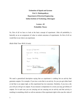
  • 1. Estimation of Signals and Systems Prof. S. Mukhopadhyay Department of Electrical Engineering Indian Institute of Technology, Kharagpur Lecture - 02 Probability Theory So, first of all we have to look at the basic concept of experiment. After all probability is basically an an an assignment of value to certain outcomes of experiments. So first of all we would like to see what is an experiment. (Refer Slide Time: 00:01:16 min) We need a generalized description saying that an experiment is nothing but an activity that generates outputs. For example, if you toss a coin that is an activity. So you you get either head or tail that is an output right, so this experiment has two outcomes. Similarly, if you toss a die you will you will get six outputs. If you measure a temperature in a room you may get infinity of outputs. So in each case you are carrying out are carrying out an activity and that activity is resulting in something which we call an outcome of the experiment right in this case the value of 1
  • 2. the temperature and there may be a there maybe a number of outcomes of an experiment that number maybe finite, it maybe countably infinite or it may be uncountably infinite there is a there is a distinction between countably infinity and uncountable infinity. For example, the the number of integers are countably infinite. It is it is an infinite set but you can still count them while the number of reals are uncountably infinite because if you take any two reals between those two reals you you will again get an infinite number of reals so so therefore it is a different it has to be a higher order of infinity right. So in our case we are we are now taking a rather generalized view of probability than what we probably learnt in school so we are we have to we have to encompass is we are mainly going to be dealing with real variables so we have to deal with experiments which throw an infinity possibly an uncountable infinity of outcomes right. So so example could be coin tossing or die throwing whatever. Now a single performance of an experiment is generally called a trial. So you can perform any number of trials of that experiment; you measure the temperature on seven days you have performed seven trials right that is it that is a trial. (Refer Slide Time: 3:43) 2
  • 3. Now now we come to an event. An event is actually a slightly more complex entity than an outcome right. It is it is actually a generalized entity. For example, if you throw a die right, there are how many outcomes possible distinct possible outcomes? 6 right but at the same time you can of these six you can define another outcome or event saying that... in this case suppose you define that that the that the face that comes up is going to be even. See if you define it that way then this event which says that if you throw a die the outcome is that the face that comes up is going to be even is 2, 4 and 6. So it now it is now an event which consists of a set of outcomes okay. So in general an an outcome may not be the lowest level things that can happen it can also be subsets of possible outcomes or events. So basically events are sets of outcomes and sometimes sometimes we say that outcomes are outcomes are elementary events, we can also say that elementary events, they are the set of distinct things that can happen right. So these are this is terminology. (Refer Slide Time: 5:20) So now having understood the basic concept of an experiment let us see the definitions of probability. 3
  • 4. (Refer Slide Time: 00:05:40 min) We learnt a definition which we in in school okay which says that if you perform n trials of an experiment and if you are interested in in an event A right and if out of source n trials there are n number of cases where A occurs then probability of A is defined as limit of n tending to infinity nA by n that is the relative frequency of occurrence of an event in a... generally we say in a large number of trials right. So if you toss a coin we say that if you have a fair coin then the probability of a of a of a of a head occurring is 0.5. Now does it mean that if you if you toss a coin twice you will get once head and once tail? No. So it is expected that that if you go on tossing the coin in a in a in a fair manner then for very large n this n head by total number of tosses will approach 0.5 this is an this is an idea right. So so this is what is known as the so-called the relative frequency definition of convention. This is called the relative frequency nA by n. 4
  • 5. (Refer Slide Time: 7:12) Now one good thing about this this definition is that it it it it gives a sense of probability that is actually you know how many times something that we are looking for is occurring, that is a that gives our our our equity physical sense of probability that is a good thing. But at the same time, you know, I mean, Mathematicians are very very abstract and logical people who do not care too much for I mean physical cases so they would say that: no no, what is this? First of all what is the use of this definition? Because if you are if you are talking of physics can you really verify this limit (Refer Slide Time: 7:47), you cannot because then you have to do it infinite number of trials and then without performing an infinite number of trials how do you know even that this limit even exists; you do not know. So anyway you are using a hypothesis that that if you perform an infinite number of trials it will this this it means this ratio is quantity nA by n will approach a limit this is your hypothesis you cannot verify it. So based on that hypothesis you are you are defining this probability. So they would say that no no why all this... let us not assign any let us not find out that is how this how we are assigning these numbers P. But let us say that if we assign these if we assign what is I mean if we define a function probability by which we assign some numbers to some events then what should be the properties that these numbers would be. Then then whether you assign these numbers based on your belief or whether you assign the numbers actually by doing a 5
  • 6. large number of experiments that is even. But if you want to if you want to assign a a a sense of probability then waste a logical deduction system on that then these definition should should obey certain what are known as axioms. So any assignment how you have done that assignment whether you knew it or whether you heard it or or whether you found it in your experience that is immaterial. But if you define those numbers then they must be defined following some rules. And any number, any assignments be which obeys those rules is a is a is a valid probability assignment okay without knowing too much about how this arrive at it because they are not interested in that. In fact, if you read modern books on probability it will widely argue that this is the this is the more elegant and better way of defining probability rather than on relative frequency okay. (Refer Slide Time: 00:09:50 min) So here comes an axiomatic definition. It is called axiomatic because it is a definition which which will which has to satisfy certain axioms okay. So so before defining that people generally define what is known as the probability space. Do not get intimidated by terms. They are they are they are really simple quantities, only mathematicians are you know very vigorous so they would like to give terms to everything and would leave leave leave leave nothing unstated and things 6
  • 7. like that so some of them will be complicated but it makes sense intuitively. So, first of all they will define a set called S which is the set of all possible outcomes. So if you if you toss a coin this this S is going to be 1, 2, 3, 4, 5, 6; 1comma, so for tossing a coin this S this set is going to be 1 2 3 not coin 5 and 6 this is your set S okay and events are all subsets of S including the null set that is if you take... so what you what you mean by all subsets of S, you get something like B null set or then you have all 1, 2 and so on then you have all 1, 2 2, 3 or 1, 3 and all and then you have 1, 2, 3 so all subsets of S including S all them are possible events right. S is generally called a certain event because what is what is the meaning of an event? When you say 1, 2 what is the event the event is that either a 1 or a 2 occurs. If if a 1 or 2 occurs then we say that the events this particular event has occurred. So obviously S is called the certain event because S contains all outcomes so it must occur. And phi is called the impossible event because if you toss a die one of them will come so the empty set cannot come. Therefore it is a it is an impossible event. Even but that... okay by by by by terminology it is impossible and these are the elementary events okay. So now, what is a probability? Probability is simply defined as a mapping. So what is... it is a mapping from 2 to the power S 2 to the power S is again a notation it means the it is nothing it means nothing but all subsets of S it is the set of all subsets of S, it is called the power set of S. So it is a mapping from the set of all subsets of S 2 things 1 and 0, what does it mean? That means if you take any subset of S, suppose I say that a a a number y equal to f x is a mapping from reals to reals what does it mean? It means that if you choose a real case through the mapping you can get another real y right. So in this case the set this is the this is the domain of the function (Refer Slide Time: 13:09) that means if you choose any subset of S then that subset you can assign a value, it must lie between the on the real line, it is the closed interval 0 and 1 so it has to be assigned a value between 0 and 1 such that you cannot assign it in any way you like such that for all events in A this assignment should be must be greater than equal to 0 because it is assigned 0 and 1 so it satisfies you if you consider it as a mapping between 0 and 1. 7
  • 8. (Refer Slide Time: 13:46) So the so the probability of an of an event cannot be negative, it must be greater than or equal to 0. Secondly, the you must assign it in a such a manner that the that the probability of S must be one, that must be that must be followed; you cannot make any other assignment for the event S. And if you have two events such that their their intersection is null that is they are exclusive events; for example, one event is 1 or 2 occurs, another event is 3 or 4 of S these are exclusive events. If if they are exclusive events then then the probability of A union B must be the sum of probability of A plus probability of B. You must assign numbers to the sets in such a manner. These three axioms must be satisfied and any assignment any assignment of a function which satisfies these three is a is a valid probability assignment. Then after after satisfying these three how you exactly assign numbers to the sets is actually your business. This you can do it on on on various things right. So... and well this is (........14:59) extendible for a countable infinity of sets. That is if you have mutually exclusive sets A 1, A 2,.......... up to n countably if A 1 A 2 dot dot dot countable exclusive sets then probability of A 1 union A 2 union dot dot dot is probability of A 1 plus probability of A 2 and so on. So this result which I have taken for two sets for simplicity can be extended for a countable union of sets but not for an uncountable... these are very there are there are these are some very subtle mathematical details which which I will skip which I will not even 8
  • 9. mention because they will require some understanding of especially real analysis; I mean you have to know what are what are open sets, what are closed sets, what is their convergent, what is what is uncountable units and countable units so they are they are actually very I mean very technical matter so and they hardly ever matter so so so some of those things I will if you are really interested you should read a vigorous book on probability. So this is just for mentioning because after all we are we are interested in probability spaces which have an infinite number of outcomes so we have to always keep track of this. (Refer Slide Time: 00:16:20 min) Now, incidentally the conventional definition of probability based on based on relative frequency satisfies the axioms. For example, nA by n is greater than 0 because nA is greater than or equal to zero and n is greater than 0. So so therefore A by n must be greater than... must be greater than or equal to 0 right nA is greater than or equal to 0 and n is greater than 0. So therefore the the relative frequency definition satisfies the first axiom. Obviously for obviously if for the for for the total set S nS equal to n because anytime you try S is going to be satisfied so therefore S by n equal to 1 so the second second axiom is also satisfied. Similarly, you will find that that that if the events are exclusive then n of A union B is nothing but nA plus nB because there is no common, A and B cannot occur together. So therefore nA nA 9
  • 10. union B by n is simply equal to nA by n plus nB by n. So this is probability of A, probability of B. So the so the relative frequency definition is just one of such probability assignments. There could a there could an infinite number of other ways of assigning probabilities to events. But the... where the relative frequency definition which we studied in school happens to satisfy the axioms; right. So it is a generalization actually okay. Similarly, we have now we we sometimes will come to this theme that two events if they are equal obviously probability of A will be equal to probability of B because it is a function right. But probability of A equal to probability of B it never implies that A is equal to B; obviously probability of 1 and 2 or probability of 3 and 4 are same doesn’t meant that the set 1 and 2 is equal to the set 3 and 4 no question. But you can have a set you can have a you can have two sets which are equal only in the sense of probability. So you can say that they are equal with probability 1 right, what does it mean? It means that the the probability of say we we we have learnt about Venn diagrams. So this is A and this is B right? So what is A union B? A union B is... what is A union B? Minus A intersection B it is this part, right? So, if the... so so this is another event because it is a set. So if the probability of this is 0 then the two events are supposed to be equal with probability 1 means what? It means that the the event set may occur that is the set A and the set B are are actually different, I mean as they have been defined they are different but these events cannot occur because it because of the probability of this hash part is 0 which means that these events cannot occur, only this part can occur (Refer Slide Time: 20:07). See if these events cannot occur as far as probability is concerned you say A and B are equal. Are you following? What I am saying is that see the A and B obviously are different sets as they as... they are not same, so how they are different they are actually different in this part because these are the elements which occur in A but do not occur in B. Similarly these are the elements which occur in B but do not occur in A. Now if the probability of these events are are 0 it means that these these elements where the set nB actually differ from each other they do not occur, they are probably 0. So only only this part occurs which is common to A and B. So, as far as the probabilistic 10
  • 11. condition is concerned A and B sets are equal. So it is equal with probability 1, it is equaling the sets of probable, they are not equal as such right. (Refer Slide Time: 00:21:19) So now now the thing is that if you come to infinite sets then we will find that you can... we have seen that how can you define a probability, you can define... for example, if you have set A is equal to 1, 2, 3 then you can define PA is equal to P 1 plus P 2 because they are they are mutually exclusive events plus P 3 right; so in this way you can take you can assign probability to elementary events, you can simply add them up to get the probability of the event right. But that but the point is that when can you do it, can you do it all cases? 11
  • 12. (Refer Slide Time: 22:24) For example, if if your probability space is the real line then can you do it? I mean it turns out that these are some again some some mathematical details, it turns out that the assignment of probability actually cannot be done to all subsets of points in the real line, this is why Mathematicians are great that that is they have they have they have been able to find out that there are some real combination of points you can take on the real line on which you cannot define probability so so that is why they will they will try to try to (circum.......22:56) this problem and and they will define... they will not define probability of elementary events, okay. That is why when you have when you have a real line you do not define probability of a point it is not defined, what is only defined is probability of intervals. Now intervals are always sets of points right. So so how do you define probability for the when my when my probability space is real line let us say. You can you can easily extend it to multiple dimensional space, real line is one dimensional space okay, so how do you do that; you first define a function called alpha x for any value of x such that it is greater than 0 and integral of minus infinity to infinity alpha is dx is 1. 12
  • 13. (Refer Slide Time: 23:47) That is if you integrate the function alpha over the real line from minus infinity to plus infinity it will be 1 and then once you have defined this function then you define probability in this fashion. You say that the probability of x is less than or equal to x i. The probability that a value that if if I if I measure the temperature of this room the the probability that it will be less than 25 degree centigrade is okay. So we can on the real line we can only make such statements, we cannot make a statement that what is the probability that the that the temperature of this room is going to be 25.000000 this statement actually mathematically does not make sense. So you can say what makes sense is what is the probability that this that the temperature is going to be between 25 and 25.001 that makes sense. But what is the probability that the temperature is going to be 25.00 is not a well-posed thing. So so what they say so so you define probability like this that define probability x less than or equal to x i is minus infinity to x i of alpha x to x i this is how it is defined, this is how the probability is defined. So so now... and and if you define what is the probability that x is less than or equal to x 2 and greater than or equal to x 1 that is in this case this is x 1 this is x 2 (Refer Slide Time: 25:23) so what is the probability that if you perform an experiment or a trial the outcome of x is going to be a value in this range that is integral of x 1 to x 2 alpha x dx you you did get the function of alpha x of alpha x 1 to x 2 obviously because when x is less than or equal to x i it means x is 13
  • 14. greater than or equal to minus infinity less than or equal to x i. So when you have... so you you can actually cast this in this form right. So so you define probability in terms of integral and therefore this function is called a probability density function. So the so the functions that you see for example, the normal distribution they are all probability density functions. (Refer Slide Time: 26:19) If you want to have a probability of a normal variable you will have to integrate the normal distribution then you will get the probability that are that are normal normal in distributed variable is going to be related to that alright. And you can also define other kinds of internals. For example, you can take an you can take an union of such internals. If you want to define that what is the probability that x is greater than 2 so you take what is the probability that x is less than or equal to 2, so 1 minus that will be the probability that x will be greater than 2. So you can define all kinds of subsets which are which maybe which maybe joint, which may separate all kinds of things using this definition and you may also like to verify that whether it satisfies the axiom. Any definition of probability that you make must satisfy those axioms. [Conversation between student and professor: 27:18 – 27:19] Sir, why are we taking the intervals of from minus infinity to 0? 14
  • 15. That is because... actually suppose yes, suppose we we take the case of measurement of the temperature why should we consider minus infinity, I mean after all especially for temperature there is there is there is nothing called minus infinity it is minus 273. Something so it is it is it is even physically it is not minus infinity. So in such a case you can always assume, see this is a generalized definition you can always assume that alpha x is equal to 0 for all x less than minus 273. so you start your alpha function, if you want to... even if you want to take a finite range you need not, practically speaking you need not but if you want to deal with a finite range simply make the function alpha zero beyond that range that is how, you understand what I am saying. So so... [Conversation between student and professor: 28:15 – 28:19] Why cannot you do... we take minus infinity to plus infinity sir? No, minus infinity plus infinity is is 1 that means, see we are... what are we trying to say, if you take minus infinity to plus infinity that means you are saying that what is the probability that x is less than or equal to plus infinity. Suppose you put plus infinity here what does it mean it means that what is the probability that it is less than or equal to plus infinity. So since since x is a real variable it is it is always going to be less than or equal to plus infinity so its probability is 1, that is how we have defined it so that if this is satisfied we have we have chosen the alpha function such that this happens right. So the so the integral under the under the normal curve must (inaug.......29:01) to 1 from minus infinity to plus infinity right. 15
  • 16. (Refer Slide Time: 00:28:52 min) So now we come to the case of I mean a very interesting case of conditional probability okay; that is the whole idea is that we when we when we assign when we evaluate probabilities of variables they may they may differ if we if we somehow have prior information about other things in its environment, right? So this notation says that: A is an event and M is another event of my probabilities case. Now what is the probability of A given that M has occurred? So you are told... so what is the probability of range on a given day at... you will say maybe you said 0.3 something that is you will find large number of n’s you will say you see the number of (...................00:30:16). 16
  • 17. (Refer Slide Time: 29:13) Now if I tell you that what is number of what is probability of rain given that it is a month of July once you are given that is the month of July the probability of rain on even day has to change right that is conditional probability. so the probability of an event A conditioned on another event M right and because because whenever we evaluate probabilities of events we should exploit all all information that we have already about other events and then we will be able to obtain the best the the best judgment about this probability, right. So the conditional probability of probability of A given M is defined as probability of A intersection M and probability divided by probability of M; why? Why is this definition because after all what is the probability of say let us take our example. So probability of it being the month of July and it rains in (( )) (00:31:37). Suppose M is the probability that this is the month of July and of course I do not know whether we should say what is the probability that is the month of July. But anyway let us take this example, this is that suppose there are I have I did not write that example; suppose we have a two child family, you consider two child families okay. So what is the probability that both the children are daughters. 1/4th, 1/4th, right. So obviously because what does my sample say, it is SS sorry, okay I will write BB GG BG and GB these are the events that can occur. 17
  • 18. Now of this what is A? A is B. Now from this how can you say that this is one fourth? 1 by 4 yes he is saying one fourth why why you are saying one fourth? Have we yet mainly mainly probability assignment from the set of samples from the set of events to the real line we have not yet made. He is... so, when he says 1/4th he is actually making an making an assumption, he is making an assumption that the that the probability of of a boy or a girl being born is actually the same as they are independent events, he is making that assumption; under that assumption only this probability is that is these four events are all equally likely that he is assuming that is why he is saying that this it is 1/4th right. So, fine, I mean we often make that assumption that they are equally like. So if if it is equally likely then then it is 1/4th. (Refer Slide Time: 34:52) Now what is the probability that you will get both daughters given that you already have a daughter; given that the first child is a daughter what is the probability that you will get two daughters? 18
  • 19. Now let us see, so probability of A given the... Now what is the probability that you have that the first child is a daughter, what is that set? It is GG and G, B this is the event that the first child is a daughter. What is the probability of this event? Half. So now we can say that what is the probability of A given C? It is probability of... no we are talking about... [Conversation between student and professor 35:14 – 35:17] (Refer Slide Time: 35:41) Boy. We are talking about GG, sorry if we I write if if we have this... no we are talking about GG right, so what is the probability of what is the probability of A given C, so it is what, it is 1/4th divided by ½, equal to ½. So the probability of getting two daughters given that you are you already have one daughter is is half as we said right. So it is interesting to see that now you see that now you come back to our... so so this is the sense of conditional probabilities right, we are trying to utilize other information that is occurring. 19
  • 20. (Refer Slide Time: 00:36:12 min) So now for example now you you have you have immediately have certain results that if M is a subset of A then probability of A A given M is 1 can you can you see that? If M is a subset of A then probability of A given M is 1 because if M has happened then then already one of A has occurred. So once you have told that M has happened the place A itself has been satisfied so so there is no no uncertainty about it. On the other hand, if A is a subset of M then M has happened does not mean that A has happened, there can be some event, there is also this possibility that something real has occurred but that is not A. So in that case probability of A given M is probability of A by probability of M, why is it why it is probability of A and probability of M because it is supposed to be this so why it is so why it is probability of A. [Conversation between student and professor 37:26] 20
  • 21. (Refer Slide Time: 37:28) Because of subset, because of subset. If A is a subset of M then A intersection M is A so probability of A by probability of M. Note that it is greater than equal to probability of A because probability of M must be less than or equal to 1. So you see that by incorporation of this additional additional information that that M has occurred, the probability of A that you are now now computing has increased, right? So if you already know that some part of it has occurred then the probability of the overall event A occurring increases, right. And you of course you can always verify that conditional probability mapping this probability mapping also satisfies the axioms again because why; again probability of A given M is is obviously greater than or equal to 0, right. First of all note that this is defined if probability of M is not equal to 0. If probability M is equal to 0 this probability of A is undefined. So you cannot talk about probability of A given M when probability of M is 0 because it makes no sense right. So so therefore obviously probability of A by M greater than or equal to 0 and probability of S upon M is 1, why because all subsets because M will be less than (( )) (00:39:05) subset of S for, I mean whatever if M is so it is 1 so that is satisfied and probability of A union B given M is probability of A given M plus probability of B given M. 21
  • 22. (Refer Slide Time: 39:21) Because probability of A union B given M let us just work out... is equal to what is equal to probability of A union B intersection M divided by probability of M is equal to what is equal to probability of A intersection M union B intersection M by probability of M. Now since A and B are mutually exclusive events so therefore A intersection M and B intersection M are also exclusive events. So therefore probability of A intersection M union B intersection M is probability of A intersection M plus probability of B intersection M by probability of M. So it will be equal to probability of A intersection M by probability of M plus probability of B intersection M by probability of M which is this. So you see that this conditional probability mapping is is itself a probability, it satisfies the axiom. Whenever you make a make a new way of defining probability it must map the axioms right so that is that. Now we have what we call there are two very interesting theorems: one theorem is called the total probability theorem. So total probability theorem says that probability of... if you have an event B and if you have a partitioning of S, what does it mean by partitioning of S? Means that you have sets A 1 up to say A n such that A 1 intersection rather A i intersection A j is null 22
  • 23. whenever i is not equal to j and union of A i is equal to S overall i, what does it mean? That if each sets are are disjoint so A i intersection A j is the null set there is there is there is no common element between these sets and if you take all the sets together it will make the set S. If you take union of the sets you will get this S so such a thing is called a partition. (Refer Slide Time: 40:44) So if you have a B any event B and the partitioning of the set A then you can write that probability of B is equal to probability of B given A 1 into probability A 1 plus probability of B given A 2 probability of A 2 plus in the finite case you can write probability of B given A n is the probability of A n this is called the total probability theorem. It is rather simple to prove because what is this after all, this is probability of B intersection A 1; similarly, plus probability of B intersection A 2 right? 23
  • 24. (Refer Slide Time: 41:59) Now since these are disjoint so you can write it is probability of B intersection union A i because these are disjoint we want A 2. So whenever they are disjoint you can take union here because this plus becomes union of the set is equal to P of B intersection S because union A i is S is equal to probability of B because B intersection S is nothing but B. So so this is the total probability theorem and based on that and we will end here today because you have another class we have the celebrated Bayes theorem which says that probability of A given B is nothing but probability B given A into into probability of A divided by probability of B. So we can also write it as probability of B given A into probability of A plus and if you if you have instead of A if you have for example if you have n number of A’s then probability of A i given B can be written as probability of B given A i into probability of A i 24
  • 25. (Refer Slide Time: 43:56) [Conversation between Student and Professor – Not audible ((00:44:54 min))] Probability of A given... what time is the class? 11:30 is our class okay so okay we will do that, this is this the Bayes theorem for two variables. So so see that I am I am I am in this theorem I am able to calculate probability of A given B in terms of probability of B given A, this is rather useful I mean you are taking one to the other side. This theorem is widely used in various context of probability. So we will stop here today. 25
  • 26. (Refer Slide Time: 45:33) So we basically reviewed some some elementary concepts of probability and we continue with the basic framework in which probability is discussed for infinite and finite probability spaces. Thank you. 26