to perform 3 tasks that will generate 3 data sets, which are as follows: (a) Dataset 1: Student data; (b) Dataset 2: Car data; and (c) Dataset 3: Employee's details. Explore and simulate the built-in functions of a spreadsheet app for data cleaning.

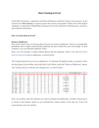
1. Data Cleaning in Excel
Excel Data Cleaning is a significant skill that all Business and Data Analysts must possess. In the
current era of data analytics, everyone expects the accuracy and quality of data to be of the highest
standards. A major part of Excel Data Cleaning involves the elimination of blank spaces, incorrect,
and outdated information.
How to Clean Data in Excel?
Remove Duplicates
One of the easiest ways of cleaning data in Excel is to remove duplicates. There is a considerable
probability that it might unintentionally duplicate the data without the user's knowledge. In such
scenarios, you can eliminate duplicate values.
Here, you will consider a simple student dataset that has duplicate values. You will use Excel's
built-in function to remove duplicates, as shown below.
The original dataset has two rows as duplicates. To eliminate the duplicate data, you need to select
the data option in the toolbar, and in the Data Tools ribbon, select the "Remove Duplicates" option.
This will provide you with the new dialogue box, as shown below.
Here, you need to select the columns you want to compare for duplication. Another critical step is
to check in the headers' option as you included the column names in the data set. Excel will
automatically scan it by default.

2. Next, you must compare all columns, so go ahead and check all the columns as shown below.
Select Ok, and Excel performs the operations required and provides you with the data set after
filtering out the duplicate data, as shown below.

3. In the next part of Excel Data Cleaning, you will understand data parsing from text to column.
Data Parsing from Text to Column
Sometimes, there is a possibility that one cell might have multiple data elements separated by a
data delimiter like a comma. For example, consider that there is one column that stores address
information.
The address column stores the street, district, state, and nation. Commas separate all the data
elements. You must now divide the street, district, state, and nation from the address columns into
separate columns.
Excel's inbuilt functionality called "text to column" can achieve this. Now, try an example for the
same.
Here, you have the car manufacturer and the car model name separated by space as the data
delimiter. The tabular data is shown below.

4. Select the data, click on the data option in the toolbar and then select "Text to Column", as shown
below.
A new window will pop up on the screen, as shown below. Select the delimiter option and click
on "next". In the next window, you will see another dialogue box.

5. In the new page dialogue box, you will see an option to select the type of delimiter your data has.
In this case, you need to select the "space" as a delimiter, as shown below.

6. In the last dialogue box, select the column data format as "General", and the next step should be
to click on the finish, as shown in the following image.
The final resultant data will be available, as shown below.

7. Followed by Data parsing, you will learn how to delete all formatting.
Delete All Formatting
Another good way of cleaning data in excel is to ensure even formatting or, in some cases, even
removing the formatting. The formatting can be as simple as coloring your cells and aligning the
text in the cells. It can be a logical condition applied to your cells using Excel's conditional
formatting option from the home tab.
However, in situations where you wish to remove the formatting, you can do it in the following
ways. First, try to eliminate the regular formatting. In the previous example, you took the case of
car manufacturers and car models data tables with heading cells colored in blue, and the text was
center aligned.
Now, use the clear option to remove the formats. Select the tabular data as shown below. Select
the "home" option and go to the "editing" group in the ribbon. The "clear" option is available in
the group, as shown below.

8. Select the "clear" option and click on the "clear formats" option. This will clear all the formats
applied on the table.
The final data table will appear as shown below.

9. Now, you must learn how to eliminate conditional formatting for cleaning data in Excel. This
time, consider a different sheet. You must use the student's details sheet, which includes
conditional formatting in Excel.
To eliminate conditional formatting in Excel, select the column or table with conditional
formatting as shown below.
Then navigate to "Home", and select conditional formatting.
Then in the dialogue box, select the clear rules option. Here, you can either choose to eliminate
rules only in the selected cells or eliminate rules from the entire column.

10. After you eliminate all conditions, the resultant table would look as follows.
You can always use a shortcut method to eliminate the conditional formatting in Excel. It is by
pressing the sequential combination of the following keys as follows.
ATL + E + A + F

11. Next, you will learn about Spell Check.
Spell Check
The feature of checking the spelling is available in MS Excel as well. To check the spellings of
the words used in the spreadsheet, you can use the following method. Select the data cell, column,
or sheet where you want to perform the spell check.
Now, go to the review option as shown below.
Microsoft Excel will automatically show the correct spelling in the dialogue box, as shown
below. You can replace the words as per the requirement as shown below.

12. The final reviewed data table will like the one below.
In the next segment, you will learn about changing the text case.
Change Case - Lower/Upper/Proper
You can manipulate the data in the Excel worksheet in terms of character cases as per the
requirements. To apply case changes, you can follow the following steps.
Select the table or columns that need the case to be changed, as shown below.

13. Select the cell next to the column and apply the formula as per the requirement, as shown below.
=UPPER(cell address) - for Upper case conversion
=LOWER(cell address) - for Lower case conversion
=PROPER(cell address) - for Sentence case conversion
Now, you can drag the cell to the last row, as shown below.

14. The final data table will appear as shown below.
Now that you learned spell check, in the upcoming section of Excel Data Cleaning, you will
learn how to Highlight Errors in an Excel spreadsheet.
Highlight Errors
Highlighting errors in an Excel spreadsheet is helpful to find or sort out the erroneous data with
ease. You can do error Highlighting with the help of conditional formatting in Excel. Here, you
must consider the student data set as an example.

15. Imagine that you are interviewing all the students. There are eligibility criteria. You can shortlist
the students if they have 60% aggregate marks. Now, apply conditional formatting and sort out
the students who are eligible and not eligible.
First, select the aggregate/percentage column as shown below.
Select "Home", and in the Styles group, select conditional formatting, as shown below.
In the conditional formatting option, select the highlight option, and in the next drop-down,
select the less than an option as shown below.

16. In the settings window, you will find a slot to provide the aggregate as "60" percent and press ok.
Excel will now select and highlight cells with an aggregate of less than 60 percent. In the next
part of Excel Data Cleaning, you will understand the trim function.

17. TRIM Function
The TRIM function is used to eliminate excess spaces and tab spaces in the Excel worksheet
cells. The excessive blank spaces and tab spaces make the data hard to understand. Using the
"TRIM" function can eliminate these excessive blank spaces.
Select the data cells with excessive blank spaces and tab spaces. Now, select a new cell adjacent
to the first cell.
Apply the TRIM() function and drag the cell as shown below.
It shows the final data after the elimination of the excess space as follows.
Next, you will look at the Find and Replace function.
Find and Replace
Find and Replace will help you fetch and replace data in the entire worksheet to help in
organizing and cleaning data in Excel. Consider the employee data example.

18. Here, try to fetch an employee with the name Joe and try to rename or replace his name with John,
after changing his first name.
The "find and replace" option is present in the home ribbon in the editing group, as shown below.

19. Click on the option, and a new window will open, where you can enter the data to be fetched and
enter the text you need to replace, as shown below.
Click on "replace all", and it will replace the text. The final dataset will be as shown below.