unit wise handouts for control systems

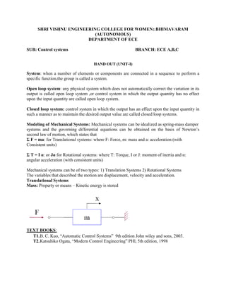
1. SHRI VISHNU ENGINEERING COLLEGE FOR WOMEN::BHIMAVARAM
(AUTONOMOUS)
DEPARTMENT OF ECE
SUB: Control systems BRANCH: ECE A,B,C
HAND OUT (UNIT-I)
System: when a number of elements or components are connected in a sequence to perform a
specific function,the group is called a system.
Open loop system: any physical system which does not automatically correct the variation in its
output is called open loop system ,or control system in which the output quantity has no effect
upon the input quantity are called open loop system.
Closed loop system: control system in which the output has an effect upon the input quantity in
such a manner as to maintain the desired output value are called closed loop systems.
Modeling of Mechanical Systems: Mechanical systems can be idealized as spring-mass damper
systems and the governing differential equations can be obtained on the basis of Newton’s
second law of motion, which states that
Σ F = ma: for Translational systems: where F: Force, m: mass and a: acceleration (with
Consistent units)
Σ T = I α: or Jα for Rotational systems: where T: Torque, I or J: moment of inertia and α:
angular acceleration (with consistent units)
Mechanical systems can be of two types: 1) Translation Systems 2) Rotational Systems
The variables that described the motion are displacement, velocity and acceleration.
Translational Systems
Mass: Property or means – Kinetic energy is stored
TEXT BOOKS:
T1.B. C. Kuo, “Automatic Control Systems” 9th edition John wiley and sons, 2003.
T2.Katsuhiko Ogata, “Modern Control Engineering” PHl, 5th edition, 1998

2. UNIT II-TRANSFER FUNCTION REPRESENTATION
Transfer Functions:
It is defined as the ratio of the Laplace transform of output (response) to the Laplace transform of
input (excitation) assuming all the initial conditions to be zero.
Procedure for reduction of Block Diagram
Step. 1 : Reduce the Cascade Blocks
Step. 2 : Reduce the parallel Blocks
Step. 3 : Reduce the internal Feed back loops
Step. 4 : It is advisable to shift take off points towards right and summing points towards left.
Step. 5 : Repeat steps 1 to step 4 until the simple form is obtained
Step. 6 : Find transfer function of the over all system using the formula C(S) / R (S)
SIGNAL FLOW GRAPHS:
A signal flow graph is a diagram that represents a set of simultaneous linear algebraic equations.
Guidelines to Construct the Signal Flow Graphs:
1) Arrange the input to output nodes from left to right.
2) Connect the nodes by appropriate branches.
3) If the desired output node has outgoing branches, add a dummy node and a unity
gain branch.
4) Rearrange the nodes and/or loops in the graph to achieve pictorial clarity.

3. UNIT-III TIME RESPONSE ANALYSIS
Changes in the reference input will cause unavoidable errors during transient periods, and also
cause steady state errors.
Classification of Control Systems:
Control systems may be classified according to their ability to follow step inputs, ramp
inputs, parabolic inputs etc.
A system is called Type 0, Type 1, Type 2 …. If N = 0, 1, 2, … respectively.
Steady State Errors:
Three types of static error constants are
1) Static position error constant Kp due to unit step input.
2) Static velocity error constant Kv due to unit ramp input.
3) Static acceleration error constant Ka due to unit parabolic input which indicate the figures of
merit of control systems
Since the error constants are defined with respect to forward path transfer function G(s), the
method is applicable to a unity feedback system only.
Principle of superposition can be used if combination of the three basic inputs are present.
TEXT BOOKS:
T1.B. C. Kuo, “Automatic Control Systems” 9th edition John wiley and sons, 2003.
T2.Katsuhiko Ogata, “Modern Control Engineering” PHl, 5th edition, 1998

4. UNIT – IV STABILITY ANALYSIS IN S-DOMAIN
Stability: all roots must be negative real numbers or complex numbers with -ve real parts.”
The following statements on stability are quite useful.
i) If all the roots of the characteristic equation have –ve real parts the system is STABLE.
(ii) If any root of the characteristic equation has a +ve real part or if there is a repeated root on
-axis, the system is unstable
(iii) If condition (i) is satisfied except for the presence of one or more non repeated roots on the
-axis the system is limitedly STABLE
Routh’s Creterion:
E.J. Routh (1877) developed a method for determining whether or not an equation has roots with
+ ve real parts with out actually solving for the roots.
A necessary condition for the system to be STABLE is that the real parts of the roots of the
characteristic equation have -ve real parts. This insures that the impulse response will decay
exponentially with time.
If the system has some roots with real parts equal to zero, but none with +ve real parts the system
is said to be MARGINALLY STABLE.
It determines the poles of a characteristic equation with respect to the left and the right half of the
S-plane with out solving the equation.
TEXT BOOKS:
T1.B. C. Kuo, “Automatic Control Systems” 9th edition John wiley and sons, 2003.
T2.Katsuhiko Ogata, “Modern Control Engineering” PHl, 5th edition, 1998

5. UNIT-V STABILITY ANALYSIS IN FREQUENCY DOMAIN
Frequency response: Frequency response of a control system refers to the steady state
response of a system subject to sinusoidal input of fixed (constant) amplitude but frequency
varying over a specific range,usually from 0 to ∞.
Frequency response can be obtained as
The linear system is subjected to a sinusoidal input. I(t) = a Sin t and the corresponding output
is O(t) = b Sin (t +)
The following
quantities are very important in frequency response analysis.
M () = b/a = ratio of amplitudes = Magnitude ratio or Magnification factor or gain.
() = = phase shift or phase angle
These factors when plotted in polar co-ordinates give polar plot, or when plotted in rectangular
co-ordinates give rectangular plot which depict the frequency response characteristics of a
system over entire frequency range in a single plot.

6. STABILITY ANALYSIS IN FREQUENCY DOMAIN :
Graphical Methods to Represent Frequency Response Data
Two graphical techniques are used to represent the frequency response data. They are: 1) Polar
plots 2) Rectangular plots.
The frequency response data namely magnitude ratio M() and phase angle () when
represented in polar co-ordinates polar plots are obtained. The plot is plotted in complex plane. It
is also called Nyquist
plot.
Rectangular Plot:
The frequency response data namely magnitude ratio M() and phase angle () can also be
presented in rectangular co-ordinates and then the plots are referred as Bode plots.
TEXT BOOKS:
T1.B. C. Kuo, “Automatic Control Systems” 9th edition John wiley and sons, 2003.
T2.Katsuhiko Ogata, “Modern Control Engineering” PHl, 5th edition, 1998

7. UNIT – VI STATE SPACE REPRESENTATION
State space technique is one of the modern approaches in the design and analysis of control
system.
state variable model :an order of differential describing a physical system can be reduced to a
set of first order differential equation and is represented in vector matrix rotation known as state
variable model.
This approach has the following advantages.
 It can be applied to linear and non-linear, time-invariant and time varying, single input
single output system and multivariable systems.
 Since it is a time domain approach, state variable model lends itself more really to
computer solution and analyses.
 State variable approach enables the designer to include initial condition.
State Variables: The state variables of a dynamic system are the smallest set of variables which
determine the state of the dynamic system.
State Space The n-dimensional space whose coordinate axes consist of the x1 axis, x2 axis, …..
xn axis is called a state space. Any state can be represented by a point in the state space.
Controllability: The concept of controllability refers to the ability of a controller to arbitrarily
alter the functionality of the system plant.
Observability: The term observability describes whether the internal state variables of the
system can be externally measured.
TEXT BOOKS:
T1.B. C. Kuo, “Automatic Control Systems” 9th edition John wiley and sons, 2003.
T2.Katsuhiko Ogata, “Modern Control Engineering” PHl, 5th edition, 1998