Abstract: The aim of the study is to reduce the size required for storage along with decreasing the bitrate and the bandwidth for the process of sending and receiving the image. It also aims to decrease the time required for the process as much as possible. This study proposes a novel system for efficient lossy volumetric medical image compression using Stationary Wavelet Transform and Linde-Buzo-Gray for Vector Quantization. The system makes use of a combination of Linde-Buzo-Gray vector quantization technique for lossy compression along with Arithmetic coding and Huffman coding for lossless compression. The system proposed uses Stationary Wavelet Transform and then compares the results obtained to Discrete Wavelet Transform, Lifting Wavelet Transform and Discrete Cosine Transform at three decomposition levels. The system also compares the results obtained using transforms with only Arithmetic Coding and Huffman Coding for Lossless Compression.The results show that the system proposed outperforms the others.

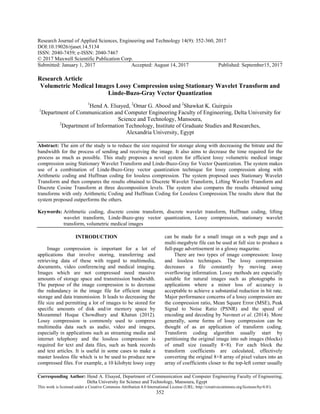
1. Research Journal of Applied Sciences, Engineering and Technology 14(9): 352-360, 2017
DOI:10.19026/rjaset.14.5134
ISSN: 2040-7459; e-ISSN: 2040-7467
© 2017 Maxwell Scientific Publication Corp.
Submitted: January 1, 2017 Accepted: August 14, 2017 Published: September15, 2017
Corresponding Author: Hend A. Elsayed, Department of Communication and Computer Engineering Faculty of Engineering,
Delta University for Science and Technology, Mansoura, Egypt
This work is licensed under a Creative Commons Attribution 4.0 International License (URL: http://creativecommons.org/licenses/by/4.0/).
352
Research Article
Volumetric Medical Images Lossy Compression using Stationary Wavelet Transform and
Linde-Buzo-Gray Vector Quantization
1
Hend A. Elsayed, 2
Omar G. Abood and 2
Shawkat K. Guirguis
1
Department of Communication and Computer Engineering Faculty of Engineering, Delta University for
Science and Technology, Mansoura,
2
Department of Information Technology, Institute of Graduate Studies and Researches,
Alexandria University, Egypt
Abstract: The aim of the study is to reduce the size required for storage along with decreasing the bitrate and the
bandwidth for the process of sending and receiving the image. It also aims to decrease the time required for the
process as much as possible. This study proposes a novel system for efficient lossy volumetric medical image
compression using Stationary Wavelet Transform and Linde-Buzo-Gray for Vector Quantization. The system makes
use of a combination of Linde-Buzo-Gray vector quantization technique for lossy compression along with
Arithmetic coding and Huffman coding for lossless compression. The system proposed uses Stationary Wavelet
Transform and then compares the results obtained to Discrete Wavelet Transform, Lifting Wavelet Transform and
Discrete Cosine Transform at three decomposition levels. The system also compares the results obtained using
transforms with only Arithmetic Coding and Huffman Coding for Lossless Compression.The results show that the
system proposed outperforms the others.
Keywords: Arithmetic coding, discrete cosine transform, discrete wavelet transform, Huffman coding, lifting
wavelet transform, Linde-Buzo-gray vector quantization, Lossy compression, stationary wavelet
transform, volumetric medical images
INTRODUCTION
Image compression is important for a lot of
applications that involve storing, transferring and
retrieving data of these with regard to multimedia,
documents, video conferencing and medical imaging.
Images which are not compressed need massive
amounts of storage space and transmission bandwidth.
The purpose of the image compression is to decrease
the redundancy in the image file for efficient image
storage and data transmission. It leads to decreasing the
file size and permitting a lot of images to be stored for
specific amounts of disk and/or memory space by
Mozammel Hoque Chowdhury and Khatun (2012).
Lossy compression is commonly used to compress
multimedia data such as audio, video and images,
especially in applications such as streaming media and
internet telephony and the lossless compression is
required for text and data files, such as bank records
and text articles. It is useful in some cases to make a
master lossless file which is to be used to produce new
compressed files. For example, a 10 kilobyte lossy copy
can be made for a small image on a web page and a
multi-megabyte file can be used at full size to produce a
full-page advertisement in a glossy magazine.
There are two types of image compression: lossy
and lossless techniques. The lossy compression
decreases a file constantly by moving away
overflowing information. Lossy methods are especially
suitable for natural images such as photographs in
applications where a minor loss of accuracy is
acceptable to achieve a substantial reduction in bit rate.
Major performance concerns of a lossy compression are
the compression ratio, Mean Square Error (MSE), Peak
Signal to Noise Ratio (PSNR) and the speed of
encoding and decoding by Navneet et al. (2014). More
generally, some forms of lossy compression can be
thought of as an application of transform coding.
Transform coding algorithm usually start by
partitioning the original image into sub images (blocks)
of small size (usually 8×8). For each block the
transform coefficients are calculated, effectively
converting the original 8×8 array of pixel values into an
array of coefficients closer to the top-left corner usually

2. Adv. J. Food Sci. Technol., 14(9): 352-360, 2017
353
contains most of the information needed to quantize and
encode the image with little perceptual distortion.
The resulting coefficients are then quantized and
the output of the quantized issued by a symbol
encoding technique to produce the output bit stream
representing the encoded image by Samra (2012). The
transformation coefficients are calculated using
different discrete transforms such as discrete cosine
transform, discrete wavelet transform, discrete lifting
wavelet transform by Kaur and Lalit (2012) and
stationary wavelet transforms by Nema et al. (2012).
The vector quantization is a classical quantization
technique for signal processing and image compression,
which allows the modeling of probability density
functions by the distribution of prototype vectors. The
main use of Vector Quantization (VQ) is for data
compression by Mukesh et al. (2013) and Vlajic and
Card (2001). It works by dividing a large set of values
(vectors) into groups having approximately the same
number of points closest to them. Each group is
represented by its centroid value, as in the Linde-Buzo-
Gray algorithm by Amin and Amrutbhai (2014). The
density matching property for vector quantization is
powerful, especially in the case for identifying the
density of large and high dimensioned data. Since data
points are represented by their index to the closest
centroid, commonly occurring data have less error and
rare data have higher error. Hence VQ is suitable for
lossy data compression. It can also be used for lossy
data correction and density estimation. The
methodology of vector quantization is based on the
competitive learning paradigm; hence it is closely
related to the self-organizing map model. Vector
Quantization (VQ) is used for lossy data compression,
lossy data correction and density estimation by Amin
and Amrutbhai (2014). The extremely fast growth of
data that needs to be stored and transferred has given
rise to the demands of better transmission and storage
techniques. Lossless data compressions categorized into
two types are: models & code and dictionary models.
Various lossless data compression algorithms have been
proposed and used. Huffman Coding, Arithmetic
Coding, Shannon Fano Algorithm, Run Length
Encoding Algorithm are some of the techniques in use
by Maan (2013) and by Kumar et al. (2015). In the case
of multimedia data, the perceptual coding transforms
the raw data to a domainthat more accurately reflects
the information content.
In this study, a novel scheme for lossy compression
of the volumetric medical images is suggested based on
Stationary Wavelet Transform and a combination of the
Linde-Buzo-Gray Vector Quantization that results low
computational complexity with no sacrifice in image
quality and Arithmetic coding and Huffman coding for
lossless compression. The execution of the suggested
algorithm has been compared with some other common
transforms such as Lifting Wavelet Transform by Al-
Rababah and Al-Marghirani (2016), Discrete Wavelet
Transform by Gopi and Rama Shri (2013) and Hadi
(2014) and Discrete Cosine Transform for lossy
compression and by Hadi (2014) and Prabhu et al.
(2013) and Stationary Wavelet Transform for lossless
compression by Anusuya et al. (2014).
MATERIALS AND METHODS
This study was conducted on 2016 and in the
Department of Information Technology, Institute of
Graduate Studies and Researches, Alexandria
University, Egypt.
Stationary wavelet transform: The Stationary
Wavelet Transform (SWT) is a recent type of wavelet
transform family that is similar to the Discrete Wavelet
Transform (DWT). It is designed to overcome the lack
of translation-invariance in the Discrete Wavelet
Transform by suppressing the process of down-
sampling and up-sampling in the DWT. This means that
SWT is translation-invariant and is designed by
upsampling only the filter coefficients by a factor of 2(j-
1)
in the jth
level of the algorithm. SWT follows an
inherently redundant scheme as each of its output levels
contains the same number of samples as the input. For a
decomposition of N levels there is a redundancy of N in
the wavelet coefficients. The two dimension WT
decomposition scheme is illustrated in Fig. 1 by Nema
et al. (2012). These sub-band images would have the
same size as that of the original image because no
down-sampling is performed during the wavelet
transform process.
Linde-Buzo-gray vector quantization: Vector
Quantization (VQ) is a lossy data compression method
based on the principle of block coding. The Vector
Quantization technique is made to develop a dictionary
of fixed-size vectors, called code vectors. A vector is
usually a block of pixel values. A given image is
separated into non-overlapping blocks called image
vectors. Then each is determined in the dictionary. The
dictionary index is used as the encoder of the original
image vector. VQ is the most powerful quantization
technique used for the image compression. The image
Vector Quantization includes four stages: vector
formation, training group selection, codebook
generation and quantization by Mittal and Lamba
(2013) and Amin and Amrutbhai (2014).
Generalized Lloyd Algorithm (GLA) is also called
the Linde-Buzo-Gray (LBG) Algorithm. It used a
mapping function to partition training vectors in N
clusters. The mapping function is defined as Rk → CB.
Let X = (x1, x2, …xk) is a training vector and d (X, Y)
be the Euclidean Distance between any two vectors.
The iteration of GLA for a codebook generation is
given as follows:

3. Adv. J. Food Sci. Technol., 14(9): 352-360, 2017
354
Fig. 1: Stationary wavelet transform of an image
Step 1: Randomly generate an initial codebook CB0.
Step 2: I = 0.
Step 3: Perform the following process for each
training vector.
Compute the Euclidean distances between the
training vector and the code words in CBi. The
Euclidean distance is defined as in Eq. (1):
∑ =
−=
k
t tt cxCXd 0
2
)(),( (1)
Search the nearest code word among CBi.
Step 4: Partition the codebook into N cells.
Step 5: Compute the centroid of each cell to get the
new codebook CBi+1.
Step 6: Compute the ratio deformation for CBi+1. If it
is changed by a small enough amount since the
last iteration, the codebook may converge and
the procedure stops. Otherwise, I = I + 1 and
go to Step 3.
LBG algorithm has the local optimization problem
and the utility of each code word in the codebook is
low. The local optimization problem means that the
codebook guarantees local minimum deformation, but
not global minimum deformation by Mittal and Lamba
(2013) and Amin and Amrutbhai (2014).
LBG Algorithmic steps:
Step 1: Divide the input image into non overlapping
blocks and transform each block into vectors.
Step 2: Randomly generate an initial codebook CB0
Step 3: Initialize I = 0.
Step 4: Perform the following process for each
training vector.
• Compute the Euclidean distance between all
the training vectors belonging to this cluster
and the code words in CBI by Eq. (1).
• Compute the centroid (code vector) for the
clusters got in the above step.
Step 5: Increment I by one and repeat the step 4 for
each code vector.
Step 6: Repeat the Step 3 to Step 5 till codebook of the
desired size is got.
The proposed lossy compression approach applied
SWT and LBG Vector Quantization techniques in order
to compress input images through four phases; namely
preprocessing, image transformation, Zigzag scan and
lossy/lossless compression. Figure 2 shows the main
steps of the system proposed. It shows how a matrix
arrangement gives the best compression ratio and least

4. Adv. J. Food Sci. Technol., 14(9): 352-360, 2017
355
Fig. 2: Flowchart of the proposed system
loss of the characteristics of the image through a
wavelet transform with lossy compression techniques.
The steps for the proposed system are as follows:
• Preprocessing: The preprocessing phase takes
images as input, so that the proposed approach
resizes images of different sizes to the size of 8×8
pixels then converts from RGB to grayscale.
• Image transformation: The image transformation
phase receives the resized grayscale image and
produces a transformed image. This phase uses
four types of the transforms which are: DCT,
DWT, LWT and SWT at three decomposition
levels.
• Zigzag scan: The Zigzag scan phase takes the
transformed image from a 2D matrix input and
reproduces it in a 1D matrix, so that the frequency
(horizontal + vertical) increases in this order and
the coefficient variance decreases in this order.
• Lossy Compression by Linde-Buzo-Gray Vector
Quantization
• Lossy compression technique provides higher
compression ratio than lossless compression.
Lossless compression: Lossless image compression
schemes exploit redundancies without incurring any
loss of data. Lossless image compression is therefore
exactly reversible. The lossless compression schemes
are the Arithmetic Coding and Huffman Coding by
Kumar et al. (2015).
Finally, measure the Compression Ratio (CR)
which is the ratio of size of the compressed database
system with the original size of the uncompressed
database systems. CR also known as "compression
power" is a computer-science term used to quantify the
reduction in data-representation size produced by a data
compression algorithm. Compression ratio is defined as
follows by Mozammel Hoque Chowdhury and Khatun
(2012) as in Eq. (2):
(2)
And measure also the Peak Signal-to-Noise Ratio
(PSNR) that is defined as the following formula by
Mozammel Hoque Chowdhury and Khatun (2012) as in
Eq. (3):
PSNR = 10log10 (2552/MSE) dB (3)
RESULTS AND DISCUSSION
This study introduced a novel lossy compression
on the 8-bit volumetric medical image data set using a
combination of LBG vector quantization and lossless
coding such as Arithmetic Coding and Huffman Coding
using stationary wavelet transform at three
decomposition levels and with the wavelet filter that is
the db1 filter. Then these results are compared with
other types of transforms which are DCT and DWT and

5. Adv. J. Food Sci. Technol., 14(9): 352-360, 2017
356
LWT. The performance metrics used are the
Compression Ratio (CR), Peak Signal-to-Noise Ratio
(PSNR) and the time needs to do the compression that
is called the running time. The description of the data
sets used in our experiments is shown by Gaudeau and
Moureaux (2009).
A volumetric medical image is a three-dimensional
(3D) image dataset which can be considered as a
sequence of two-dimensional (2D) images (or slices). A
direct way to perform compression on it is straight
forwardly apply a two-dimensional compression
algorithm to each slice independently. This section
shows the performance of the four discrete transforms
which are the DCT, DWT, LWT and SWT and at the
three decomposition levels with the wavelet filter that is
the db1 filter.
The performance also shows the use of lossless
compression using Arithmetic Coding and Huffman
Coding with the lossy using Vector Quantization by
LBG and without. The performance for the four
transforms is shown in Table 1 to 5.
Where the results in Table 1 show the compression
ratio, the peak signal-to-noise ratio and the running
time for the proposed system using SWT with a
combination of the LBG Vector Quantization and the
lossless coding techniques such as Arithmetic Coding
and Huffman Coding. The results in this table show that
the performance of the running time and the
compression ratio using Arithmetic Coding better than
using Huffman Coding at the same peak signal-to-noise
ratio for the three decomposition levels.
The results in Table 2 show that the compression
ratio, the peak signal-to-noise ratio and the running
time using SWT by Anusuya et al. (2014) without the
LBG Vector Quantization and using the lossless coding
techniques such as Arithmetic Coding and Huffman
Coding. The results in this table show that the
performance of the running time and the compression
ratio using Arithmetic Coding better than using
Huffman Coding at the same peak signal-to-noise ratio
for the three decomposition levels.
From Table 1 and 2 the results show the
compression ratio with the combination in the proposed
system in Table 1 better than without combination of
LBG and lossless coding in Table 2.
The results in Table 3 show also the compression
ratio, the peak signal-to-noise ratio and the running
time using DWT by Gopi and Rama Shri (2013) and by
Hadi (2014) with a combination of the LBG Vector
Quantization and the lossless coding techniques such as
Arithmetic Coding and Huffman Coding and without
the combination. The results in this table show that the
performance of the compression ratio using a
combination of the LBG Vector Quantization and the
lossless coding techniques better than without the
combination at the three decomposition levels and the
results in Table 1 is better than these results.
The results in Table 4 show also the compression
ratio, the peak signal-to-noise ratio and the running
time using LWT by Al-Rababah and Al-Marghirani
Table 1: Stationary wavelet transform, vector quantization (lbg), arithmetic and huffman coding
SWT
SWT Zigzag LBG and Arithmetic
---------------------------------------------------------------
SWT Zigzag LBG and Huffman
---------------------------------------------------------------
Image Level C.Ratio PSNR Time (Sec) C.Ratio PSNR Time (Sec)
Carotid 1 5.0818 17.1566 0.018 4.3481 17.1566 0.0467
2 5.0818 17.1566 0.0099 4.3481 17.1566 0.0039
3 5.0818 17.1566 0.034 4.3481 17.1566 0.0556
Liver_t1 1 5.8995 17.328 0.1635 4.8416 17.328 0.0879
2 5.8995 17.328 0.0212 4.8416 17.328 0.0788
3 5.8995 17.328 0.1565 4.8416 17.328 0.0777
Liver_t2e1 1 5.0073 15.9569 0.011 4.785 15.9569 0.0489
2 5.0073 15.9569 0.0121 4.785 15.9569 0.1009
3 5.0073 15.9569 0.055 4.785 15.9569 0.0343
Pad_chest 1 4.9708 19.1208 0.011 4.8301 19.1208 0.0578
2 4.9708 19.1208 0.0331 4.8301 19.1208 0.0344
3 4.9708 19.1208 0.031 4.8301 19.1208 0.0601
Aperts 1 4.9349 17.619 0.0111 4.2226 17.619 0.0517
2 4.9349 17.619 0.0556 4.2226 17.619 0.0565
3 4.9349 17.619 0.3901 4.2226 17.619 0.0989
Sag_head 1 4.8878 17.5288 0.0103 4.7517 17.5288 0.0439
2 4.8878 17.5288 0.0243 4.7517 17.5288 0.0634
3 4.8878 17.5288 0.0104 4.7517 17.5288 0.0359
Skull 1 5.0693 16.7471 0.0141 4.853 16.7471 0.047
2 5.0693 16.7471 0.0051 4.853 16.7471 0.0444
3 5.0693 16.7471 0.0043 4.853 16.7471 0.07
Wrist 1 5.2783 17.2772 0.0098 3.7996 17.2772 0.0543
2 5.2783 17.2772 0.0099 3.7996 17.2772 0.0466
3 5.2783 17.2772 0.01 3.7996 17.2772 0.066
Average 1 5.1412 17.3418 0.0311 4.5539 17.3418 0.0547
2 5.1412 17.3418 0.0214 4.5539 17.3418 0.0536
3 5.1412 17.3418 0.0864 4.5539 17.3418 0.0623

6. Adv. J. Food Sci. Technol., 14(9): 352-360, 2017
357
Table 2: Stationary wavelet transform, arithmetic and huffman coding
SWT
SWT Zigzag Arithmetic
-------------------------------------------------------
SWT Zigzag Huffman
-------------------------------------------------------
Image Level C.Ratio Time(Sec) C.Ratio Time(Sec)
Carotid 1 3.69 0.0681 2.4734 0.88
2 3.69 0.0491 2.4734 0.8879
3 3.69 0.0881 2.4734 0.69
Liver_t1 1 4.171 0.0713 2.629 0.0469
2 4.171 0.0689 2.629 0.665
3 4.171 0.0663 2.629 0.0565
Liver_t2e1 1 3.519 0.8817 2.519 0.8673
2 3.519 0.0817 2.519 0.6672
3 3.519 0.0317 2.519 0.734
Pad_chest 1 4.5612 0.029 2.2806 0.8721
2 4.5612 0.229 2.2806 0.7421
3 4.5612 0.0891 2.2806 0.933
Aperts 1 3.9922 0.0493 2.2579 0.9088
2 3.9922 0.0674 2.2579 0.9923
3 3.9922 0.0786 2.2579 0.881
Sag_head 1 3.828 0.0316 2.278 0.8996
2 3.828 0.0666 2.278 0.3346
3 3.828 0.0113 2.278 0.824
Skull 1 4.1541 0.0892 2.6771 0.8789
2 4.1541 0.0267 2.6771 0.9984
3 4.1541 0.0969 2.6771 0.8843
Wrist 1 4.1124 0.03 2.0983 0.8678
2 4.1124 0.37 2.0983 0.8666
3 4.1124 0.0119 2.0983 0.2008
Average 1 4.0034 0.1562 2.4016 0.77767
2 4.0034 0.1199 2.4016 0.7692
3 4.0034 0.0592 2.4016 0.6504
Table 3: Discrete wavelet transform, vector quantization (lbg), arithmetic and huffman coding
DWT
DWT Zigzag Arithmetic
-----------------------------------------------
DWT Zigzag LBG & Arithmetic
-------------------------------------------------------------------------
Image Level C.Ratio Time (Sec) C.Ratio PSNR Time (Sec)
Carotid 1 1.0513 0.068 1.2641 18.4991 0.0676
2 1.1716 0.0509 1.2832 18.3813 0.0125
3 1.1403 0.1351 1.2929 18.3848 0.0098
Liver_t1 1 1.2161 0.6479 1.6195 18.2978 0.0153
2 1.199 0.0462 1.3368 18.3244 0.0218
3 1.3161 0.0638 1.7161 18.3443 0.0178
Liver_t2e1 1 1.1082 0.0987 1.3161 18.0236 0.0093
2 1.2278 0.2769 2.415 17.9054 0.0339
3 1.2397 0.0374 1.3473 18.1348 0.0128
Pad_chest 1 1.2047 0.0459 2.2654 26.8882 0.0115
2 1.2278 0.0339 2.6654 26.8882 0.0121
3 1.2579 0.0389 2.1244 27.3571 0.0179
Aperts 1 1.047 0.0363 1.8754 18.5491 0.0105
2 1.2132 0.0395 1.9962 18.7252 0.0181
3 1.0711 0.043 1.9176 18.6427 0.0095
Sag_head 1 1.0801 0.0339 2.415 22.2526 0.0089
2 1.1851 0.0396 2.1157 22.4535 0.0086
3 1.2018 0.0454 2.1422 22.3508 0.0113
Skull 1 1.2278 0.0562 1.3689 17.9054 0.015
2 1.2736 0.0491 1.3229 17.9649 0.016
3 1.3195 0.0561 1.3509 18.0213 0.0101
Wrist 1 1.0756 0.2769 2.0645 27.2766 0.0121
2 1.2549 0.0601 2.0398 27.8388 0.0094
3 1.1252 0.0381 1.9393 27.7193 0.0139
Average 1 1.12635 0.15797 1.7736 20.9615 0.0187
2 1.219125 0.07452 1.8968 21.0602 0.01655
3 1.20895 0.05722 1.7288 21.1193 0.01288
DWT
DWT Zigzag Huffman
-----------------------------------------------
DWT Zigzag LBG & Huffman
-------------------------------------------------------------------------
Image Level C.Ratio Time (Sec) C.Ratio PSNR Time (Sec)
Carotid 1 1.0192 0.1765 1.0847 18.4991 0.0477
2 1.0241 0.0743 1.96 18.3813 0.0435
3 1.0904 0.071 1.047 18.3848 0.0589
Liver_t1 1 1.087 0.1771 1.1082 18.2978 0.0488
2 1.1034 0.0765 1.1179 18.3244 0.0465
3 1.0377 0.0995 1.1327 18.3443 0.0696

7. Adv. J. Food Sci. Technol., 14(9): 352-360, 2017
358
Table 3: Continue
DWT
DWT Zigzag Huffman
----------------------------------------
DWT Zigzag LBG & Huffman
------------------------------------------------------------------------
Image Level C.Ratio Time (Sec) C.Ratio PSNR Time (Sec)
Liver_t2e1 1 1.0642 0.0632 1.094 18.0236 0.0709
2 1.0663 0.064 1.8476 17.9054 0.0815
3 1.0225 0.0759 1.087 18.1348 0.0486
Pad_chest 1 1.0663 0.0671 1.9078 26.8882 0.0446
2 1.0663 0.064 1.8648 26.8882 0.0436
3 1.0619 0.0647 1.9078 27.3571 0.063
Aperts 1 1.0476 0.0676 1.5014 18.5491 0.0653
2 1.0819 0.0731 1.5678 18.7252 0.0506
3 1.0332 0.0739 1.8378 18.6427 0.0572
Sag_head 1 1.0634 0.0973 1.8476 22.2526 0.0579
2 1.0858 0.0619 1.9078 22.4535 0.0476
3 1.7901 0.0694 1.9898 22.3508 0.0598
Skull 1 1.0824 0.064 1.1277 17.9054 0.0436
2 1.0406 0.0688 1.1403 17.9649 0.05
3 1.0096 0.0909 1.1403 18.0213 0.0486
Wrist 1 1.0216 0.0815 1.8648 27.2766 0.0457
2 1.105 0.0821 1.9078 27.8388 0.0443
3 1.742 0.0857 1.8888 27.7193 0.0577
Average 1 1.0564 0.09928 1.4420 20.9615 0.0530
2 1.0716 0.07058 1.6642 21.06021 0.0509
3 1.2234 0.0788 1.5039 21.11938 0.0579
Table 4: Lifting wavelet transform, vector quantization (lbg), arithmetic and huffman coding
LWT
LWT Zigzag Arithmetic
-----------------------------------------------
LWT Zigzag LBG & Arithmetic
------------------------------------------------------------------------
Image Level C.Ratio Time (Sec) C.Ratio PSNR Time (Sec)
Carotid 1 1.3636 0.1433 1.6842 15.1588 0.0116
2 1.1636 0.1076 1.641 14.1798 0.0107
3 1.1428 0.1301 1.641 16.4423 0.0104
Liver_t1 1 1.3743 0.4263 1.641 17.5346 0.0141
2 1.2636 0.0486 1.6842 14.1617 0.0118
3 1.1228 0.0448 1.6623 19.5076 0.0074
Liver_t2e1 1 1.4327 0.0313 1.6955 16.0485 0.0069
2 1.1962 0.078 1.641 14.2502 0.007
3 1.1931 0.0601 1.4564 19.5367 0.0104
Pad_chest 1 1.3428 0.0292 1.9833 15.8712 0.011
2 1.1327 0.0338 1.7066 16.3622 0.0071
3 1.2075 0.0414 1.7066 17.6318 0.0103
Aperts 1 1.1636 0.0298 1.7066 15.3466 0.0107
2 1.1962 0.0492 1.641 13.3961 0.014
3 1.3195 0.0343 1.6202 17.3437 0.0124
Sag_head 1 1.4428 0.0636 1.7777 15.9653 0.0072
2 1.1327 0.1024 1.7297 17.3593 0.0077
3 1.1444 0.1645 1.641 20.5763 0.0077
Skull 1 1.1428 0.052 1.641 17.9075 0.0105
2 1.28 0.0766 1.6623 13.3142 0.0102
3 1.1228 0.0938 1.6842 19.4484 0.008
Wrist 1 1.2075 0.0276 1.6842 15.7742 0.0071
2 1.2075 0.0529 1.7066 16.2986 0.0104
3 1.2075 0.0276 1.6842 15.7742 0.0071
Average 1 1.3087 0.1003 1.7266 16.2008 0.0098
2 1.1965 0.0686 1.6765 14.9152 0.0098
3 1.1784 0.0782 1.6315 18.4662 0.0095
LWT
LWT Zigzag Huffman
-----------------------------------------------
LWT Zigzag LBG & Huffman
------------------------------------------------------------------------
Image Level C.Rati Time (Sec) C.Ratio PSNR Time (Sec)
Carotid 1 1.2929 0.0482 1.3934 15.1588 0.0155
2 1.1451 0.0718 1.4712 14.1798 0.0157
3 1.1228 0.0399 1.4222 16.4423 0.0165
Liver_t1 1 1.1763 0.0445 1.4065 17.5346 0.0216
2 1.1851 0.0449 1.4456 14.1617 0.0149
3 1.1531 0.0455 1.4222 19.5076 0.0177
Liver_t2e1 1 1.3333 0.0696 1.4545 16.0485 0.0143
2 1.1246 0.0601 1.4712 14.2502 0.0159
3 1.1743 0.109 1.3763 19.5367 0.0161
Pad_chest 1 1.2549 0.1238 1.3763 15.8712 0.0263
2 1.1021 0.0779 1.4545 16.3622 0.0258
3 1.0756 0.0419 1.4545 17.6318 0.0177

8. Adv. J. Food Sci. Technol., 14(9): 352-360, 2017
359
Table 4: Continue
LWT
LWT Zigzag Huffman
-----------------------------------------------
LWT Zigzag LBG & Huffman
-----------------------------------------------------------------------
Image Level C.Rati Time (Sec) C.Ratio PSNR Time (Sec)
Aperts 1 1.3195 0.07 1.4545 15.3466 0.0261
2 1.0756 0.0672 1.4712 13.3961 0.0142
3 1.0406 0.0509 1.4712 17.3437 0.0201
Sag_head 1 1.3913 0.0344 1.5555 15.9653 0.0261
2 1.1851 0.038 1.4382 17.3593 0.0186
3 1.1228 0.043 1.4712 20.5763 0.0266
Skull 1 1.1113 0.037 1.5382 17.9075 0.0222
2 1.1333 0.0749 1.4222 13.3142 0.0146
3 1.1851 0.066 1.4484 19.4484 0.0175
Wrist 1 1.1195 0.0436 1.5566 15.7742 0.0182
2 1.1531 0.0697 1.4545 16.2986 0.0196
3 1.1195 0.0436 1.5566 15.7742 0.0182
Average 1 1.2498 0.0588 1.4669 16.2008 0.0212
2 1.138 0.0630 1.4535 14.9152 0.0174
3 1.1271 0.0542 1.4594 18.4662 0.0188
Table 5: Discrete cosine transform, vector quantization (lbg), arithmetic and huffman coding
DCT
DCT Zigzag Arithmatic
------------------------------------------------------
DCT & LBG Zigzag Arithmatic
-----------------------------------------------------------------------------------
Image C. Ratio Time (Sec) C. Ratio PSNR Time (Sec)
Carotid 1.0711 0.1167 1.28 18.7433 0.0212
Liver_t1 1.1962 1.1862 1.5375 18.3015 0.0208
Liver_t2e1 1.2132 0.03 1.3333 18.8851 0.0135
Pad_chest 1.3368 0.0484 2.3703 30.3357 0.0105
Aperts 1.2278 0.0325 1.8962 19.6048 0.0139
Sag_head 1.1203 0.0285 2.0078 21.6627 0.0142
Skull 1.1743 0.0434 1.467 21.1481 0.0144
Wrist 1.2864 0.0345 2.4265 27.2516 0.0089
Average 1.2032625 0.190025 1.789825 21.9916 0.014675
DCT
DCT Zigzag Huffman
------------------------------------------------------
DCT & LBG Zigzag Huffman
-----------------------------------------------------------------------------------
Image C. Ratio Time(Sec) C. Ratio PSNR Time (Sec)
Carotid 1.0427 0.0712 1.06 18.7433 0.0445
Liver_t1 1.099 0.0845 1.2513 18.3015 0.0484
Liver_t2e1 1.0046 0.0753 1.113 18.8851 0.048
Pad_chest 1.0039 0.0773 1.8533 30.3357 0.0437
Aperts 1.0275 0.1019 1.3078 19.6048 0.0469
Sag_head 1.0178 0.1008 1.8767 21.6627 0.0424
Skull 1.0743 0.0591 1.6578 21.1481 0.0447
Wrist 1.059 0.0576 1.8533 27.2516 0.0718
Average 1.0411 0.0784625 1.49665 21.9916 0.0488
(2016) with a combination of the LBG Vector
Quantization and the lossless coding techniques such as
Arithmetic Coding and Huffman Coding and without
the combination. The results in this table show that the
performance of the compression ratio using a
combination of the LBG Vector Quantization and the
lossless coding techniques better than without the
combination at the three decomposition levels and the
results in Table 1 is also better than these results.
The results in Table 5 show also the compression
ratio, the peak signal-to-noise ratio and the running
time using DCT by Hadi (2014) and Prabhu et al.
(2013) with a combination of the LBG Vector
Quantization and the lossless coding techniques such as
Arithmetic Coding and Huffman Coding and without
the combination. The results in this table show that the
performance of the compression ratio using a
combination of the LBG Vector Quantization and the
lossless coding techniques better than without the
combination and the results in table Iis also better than
these results.
The results in Table 3 using LWT outperform the
results in Table 3 using DWT and the results in Table 3
using DWT outperform the results in Table 5 using
DCT. Then the results in Table 1 outperform the results
in Table 2 to 5 using DCT.
So, the proposed system outperforms the other
previous methods in Table 2 to 5.
CONCLUSION
This study proposes a system that works on
medical images compression by using a combination of
lossy compression through LBG Vector Quantization
and lossless compression through Arithmetic Coding. It
also used Huffman Coding for comparison and different

9. Adv. J. Food Sci. Technol., 14(9): 352-360, 2017
360
transforms which are DCT and three types of wavelet
transforms which are SWT, DWT and LWT at three
levels.
The results show that the performance depends on
the type of the transform, whether LBG was used or
not, the number of decomposition levels and the type of
the lossless coding whether it was Huffman Coding or
Arithmetic Coding.
The lossy compression approach used SWT and a
combination of the LBG Vector Quantization and the
lossless coding outperforms the other wavelet
transforms such as the DWT and the LWT and the other
transform which is DCT. The arithmetic coding gives
the best compression ratio with less time possible.
REFERENCES
Al-Rababah, M. and A. Al-Marghirani, 2016.
Implementation of novel medical image
compression using artificial intelligence. Int. J.
Adv. Comput. Sci. Appl., 7(5): 328-332.
https://thesai.org/Downloads/Volume7No5/Paper_
44-
Implementation_of_Novel_Medical_Image_Compr
ession_Using_Artificial_Intelligence.pdf
Amin, B. and P. Amrutbhai, 2014. Vector quantization
based lossy image compression using wavelets: A
review. Int. J. Innov. Res. Sci. Eng. Technol., 3(3):
10517-10523. https://www.rroij.com/open-
access/vector-quantization-based-lossy-
imagecompression-using-wavelets--a-review.pdf
Anusuya, V., V. Srinivasa Raghavan and G. Kavitha,
2014. Lossless compression on MRI images using
SWT. J. Digit. Imaging, 27(5): 594-600.
https://www.ncbi.nlm.nih.gov/pmc/articles/PMC41
71424/
Gaudeau, Y. and J.M. Moureaux, 2009. Lossy
compression of volumetric medical images with
3D dead zone lattice vector quantization. Ann.
Telecommun., 64(5-6): 359-367.
https://link.springer.com/article/10.1007/s12243-
008-0079-5
Gopi, K. and T. Rama Shri, 2013. Medical image
compression using wavelets. IOSR J. VLSI Signal
Process., 2(4): 1-6. //www.iosrjournals.org/iosr-
jvlsi/papers/vol2-issue4/A0240106.pdf?id=2036
Hadi, G.M., 2014. Medical image compression using
DCT and DWT techniques. Adv. Image Video
Process., 2(6): 25-35.
http://scholarpublishing.org/index.php/AIVP/articl
e/view/771
Kaur, P. and G. Lalit, 2012. Comparative analysis of
DCT, DWT and LWT for image compression. Int.
J. Innov. Technol. Explor. Eng., 1(3): 2278-3075.
http://www.oalib.com/paper/2172362#.WaToID6G
PIU
Kumar, G., E.S.S. Brar, R. Kumar and A. Kumar, 2015.
A review: DWT-DCT technique and arithmetic-
huffman coding based image compression. Int. J.
Eng. Manuf., 3: 20-33.
https://www.researchgate.net/publication/2825713
72_A_Review_DWT-
DCT_Technique_and_Arithmetic-
Huffman_Coding_based_Image_Compression
Maan, A.J., 2013. Analysis and comparison of
algorithms for lossless data compression. Int. J.
Inform. Comput. Technol., 3(3): 139-
146.https://www.ripublication.com/irph/ijict_spl/07
_ijictv3n3spl.pdf
Mittal, M. and R. Lamba, 2013. Image compression
using vector quantization algorithms: A review.
Int. J. Adv. Res. Comput. Sci. Softw. Eng., 3(6):
354-358.
https://pdfs.semanticscholar.org/24d2/db6db81f100
0b74246d22641e83390fb1065.pdf
Mozammel Hoque Chowdhury, M. and A. Khatun,
2012. Image compression using discrete wavelet
transform. Int. J. Comput. Sci. Issues, 9(4)1: 327-
330. https://www.ijcsi.org/papers/IJCSI-9-4-1-327-
330.pdf
Navneet, Guide and A.P.E. Mandeep Kaur, 2014.
Review: Analysis and comparison of various
techniques of image compression for enhancing the
image quality. J. Basic Appl. Eng. Res., 1(7): 5-8.
http://www.krishisanskriti.org/vol_image/02Jul201
50507114.pdf
Nema, M., L. Gupta and N.R. Trivedi, 2012. Video
compression using SPIHT and SWT wavelet. Int. J.
Electron. Commun. Eng., 5(1): 1-8.
http://www.ripublication.com/irph/ijece/01_11581-
%20IJECE__pp%201-8.pdf
Prabhu, K.M.M., K. Sridhar, M. Mischi and H.N.
Bharath, 2013. 3-D warped discrete cosine
transform for MRI image compression. Biomed.
Signal Proces., 8(1): 50-58.
http://www.sciencedirect.com/science/article/pii/S1
746809412000481
Samra, H.S., 2012. Image compression techniques. Int.
J. Comput. Technol., 2(2): 49-52.
https://pdfs.semanticscholar.org/a72b/4fbb12e3bb2
2db93f83c94589e66298c4a7e.pdf
Vlajic, N. and H.C. Card, 2001. Vector quantization of
images using modified adaptive resonance
algorithm for hierarchical clustering. IEEE T.
Neural Networ., 12(5): 1147-1162.
http://ieeexplore.ieee.org/document/950143/.