Chapter 11

Chapter 11: Chi-Square Tests
344
This chapter presents material on two more hypothesis tests for _______________ data.
One is used to determine if there is a significant relationship between _______________
variables, and the second is used to determine if the sample data come from a population
that has a ____________________________.
Section 11.1: Chi-Square Test for Independence
Remember, qualitative data result when you collect data on individuals that are categories
or names. Then you would count how many of the individuals were in a particular
category. There is a theory that there is a relationship between breastfeeding and autism.
Does breastfeeding longer decrease the risk of autism? To determine if there is a
relationship, researchers could collect the time period that a mother breastfed her child
(given as categories like none, less than 2 months, etc.) and if that child was diagnosed
with autism. In chapter 2, we learned how to make a _________________ to summarize
information for two qualitative variables. Now you want to know if each cell in the
contingency table is _______________of each other cell. Remember, independence says
that whether or not one event happens does not affect the probability of the other event
happening. In this case we want to know if the time period that a mother breastfeeds her
child has any effect on the chance that her child develops autism. If you were to do a
hypothesis test, the null hypothesis is that they are independent (the time period does not
affect the chance of a child developing autism) and the alternative hypothesis would be
that they are dependent (the time period does affect the chance of a child developing
autism). Below are the collected data organized into a contingency table.
Table #11.1.1: Autism Versus Breastfeeding
Autism
Breast Feeding Timelines
Row
Total
None Less
than 2
months
2 to 6
months
More
than 6
months
Yes 241 198 164 215 818
No 20 25 27 44 116
Column Total 261 223 191 259 934
Each of the values in the highlighted cells are the __________________. The symbol for
each observed frequency is O. The null hypothesis will say that the time period that a
mother breastfeeds and autism are independent. We need to know what we would expect
to see in each of the cells in the above table if this were true (in all hypothesis tests we
start by assuming the ________________________). From chapter 4 we know that for
independent events 𝑃( 𝐴 𝑎𝑛𝑑 𝐵) = _____________and then to get the expected count we
would take n times that probability. To estimate the probability of being in a particular
cell we will take (that cell’s row total divided by n) times (that cell’s column total divided
by n). That gives us the following formula for the expected count for each cell:
Expected count of a cell = E = 𝑛 (
𝑟𝑜𝑤 𝑡𝑜𝑡𝑎𝑙
𝑛
)(
𝑐𝑜𝑙𝑢𝑚𝑛 𝑡𝑜𝑡𝑎𝑙
𝑛
) =
( 𝑟𝑜𝑤 𝑡𝑜𝑡𝑎𝑙)∙( 𝑐𝑜𝑙𝑢𝑚𝑛 𝑡𝑜𝑡𝑎𝑙)
𝑛

Chapter 11: Chi-Square Tests and ANOVA
345
If the variables are independent, the expected frequencies and the observed frequencies
would be the same (or close enough in the sample data). The test statistic here will
involve looking at the difference between the expected frequency and the observed
frequency for each cell. Then you want to find the “total difference” of all of these
differences. The larger the total, the smaller the chances that you could find that test
statistic given that the assumption of independence is true. That means that the
assumption of independence is probably not true (we would reject 𝐻0). How do you find
the test statistic? First find the differences between the observed and expected
frequencies. Because some of these differences will be _____________ and some will be
_________________, you need to ___________ these differences. These squares could
be large just because the frequencies are large, you need to divide by the expected
frequencies to scale them. Then finally add up all of these fractional values. This is a
new test statistic call chi-square.
Test Statistic:
The symbol for Chi-Square is c2
𝜒2
= ∑
(𝑂 − 𝐸)2
𝐸
𝑎𝑙𝑙 𝑐𝑒𝑙𝑙𝑠
where O is the ______________________ and E is the _____________________
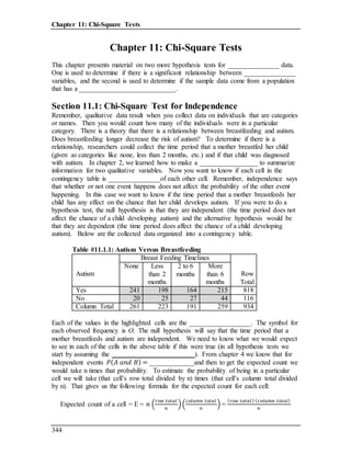
Distribution of Chi-Square
The random variable c2
has different curves on depending on something called
degrees of freedom (df)…needed when we were using tables long, long ago…
which depends on the number of row and column categories. It is skewed to the
right when the number of categories is small and gets more symmetric as the
number of categories increases (see figure #11.1.1). Since the test statistic
involves squaring the differences, the test statistic is always _______________.
Figure #11.1.1: Chi-Square Distribution
This new distribution is what will be used in the Chi-Square Independence Test. Just
as with previous hypothesis tests, all the steps are the same except for the assumptions
and the test statistic. In this case, there will not be a parameter so we will have
PHANTOMS without the P.

346
Chi-Square Independence Test (𝝌 𝟐
-Test)
1. State the null and alternative Hypotheses and the level of significance
𝐻0: the row variable and the column variable are independent
𝐻𝐴: the row variable and the column variable are dependent
Also, state your 𝛼 level here.
2. State and check the Assumptions for a hypothesis test
1.) A random sample was taken.
2.) The expected frequency for each cell is at least 5
 Check the values in matrix [B] after you run the 𝜒2
-Test
3.) 𝑁 ≥ 20𝑛 (Assume true if no N given)
3. Name the hypothesis test used
In this case the assumptions for the Chi-Square Independence Test have been satisfied.
4. Find the Test statistic
Using the TI84: You would first need to enter the observed data into matrix A
 Push 2𝑛𝑑 𝑥−1
to get into MATRIX and then push → → to get to the EDIT menu.
Push 1 for matrix [A]. You need to tell it how many rows and how many columns you
need and then enter the data in the matrix exactly how it looks in the contingency table.
 After entering the observed data, push 𝑆𝑇𝐴𝑇 → → and then scroll to see where “𝜒2
-
test” is on yourTI and then push ENTER. Next to “Observed” make sure it says [A] and
next to “Expected” make sure it says [B]
 Then scroll down and highlight “Calculate” and push ENTER
 To see the expected values you need to look at the values in matrix [B]. Push 2𝑛𝑑 𝑥−1
to get into MATRIX, push 2 to choose matrix [B] and then push ENTER
Using StatCrunch: You would first need to enter the contingency table of data like we did in
chapter 2 when we made side-by-side bar charts (there may be more categories).
 Then choose Stat, Tables, Contingency, With Summary
 Under “Select Columns” choose all columns except the first one, under “Row Labels”
choose the first column and under“Display” choose Expected Count and then click
“Compute!”
Test Statistic:
𝜒2
= ∑
(𝑜𝑏𝑠𝑒𝑟𝑣𝑒𝑑 − 𝑒𝑥𝑝𝑒𝑐𝑡𝑒𝑑)2
𝑒𝑥𝑝𝑒𝑐𝑡𝑒𝑑
5. Obtain the p-value and illustrate the meaning of the p-value and test statistic
6. Make a decision about H0
Reject 𝐻0 if the p-value ≤ a and fail to reject 𝐻0 if the p-value > a
7. State a conclusion in the context of the problem
 If you reject 𝐻0, then there is significant evidence to conclude (𝐻𝐴 in context)
 If you fail to reject 𝐻0, then there is NOT significant evidence to conclude (𝐻𝐴 in context)

347
Example #11.1.1: Hypothesis Test with Chi-Square Test
Is there a relationship between autism and breastfeeding? To determine if there
is, a researcher asked mothers of autistic and non-autistic children to say what
time period they breastfed their children. The data for 934 randomly selected
infants is in table #11.1.1 (Schultz, Klonoff-Cohen, Wingard, Askhoomoff,
Macera, Ji & Bacher, 2006). Do the data provide enough evidence to show that
that breastfeeding and autism are dependent? Test at the1% level.
Table #11.1.1: Contingency Table of Autism Versus Breastfeeding Data
Autism
Breast Feeding Timelines
Row
Total
None Less
than 2
months
2 to 6
months
More
than 6
months
Yes 241 198 164 215 818
No 20 25 27 44 116
Column Total 261 223 191 259 934
Solution:
𝐻0:
𝐻𝐴:
2. State and check the Assumptions for the hypothesis test
1)
2) Expected frequencies for each cell are greater than or equal to 5 (ie. E ³ 5).
3) No N is given, we will assume 𝑁 ≥ 20𝑛
3. Name the procedure used:
The assumptions for the _________________________________ are met.
Using the TI-84 calculator:
You need to put the data in as a matrix. Go into the MATRIX menu then
move over to EDIT and choose 1:[A]. This will allow you to type the table
into the calculator. Figure #11.1.2 shows what you will see on your calculator
when you choose 1:[A] from the EDIT menu.
Figure #11.1.2: Matrix Edit Menu on TI-84

348
The given contingency table of data has 2 rows and 4 columns (don’t include
the row total column and the column total row in your count, just enter the
part of the table that is highlighted). You need to tell the calculator that you
have a 2 by 4. The 1 X1 (you might have another size in your matrix, but it
doesn’t matter because you will change it) on the calculator is the size of the
matrix. So type 2 ENTER and 4 ENTER and the calculator will make a
matrix of the correct size. See figure #11.1.3.
Figure #11.1.3: Matrix Setup for Table
Now type the table in by pressing ENTER after each cell value. Figure
#11.1.4 contains the complete table typed in. Once you have the data in, press
QUIT.
Figure #11.1.4: Data Typed into Matrix
To run the test on the calculator, go into STAT, then move over to TEST and
choose c2
-Test from the list. The setup for the test is in figure #11.1.5.
Figure #11.1.5: Setup for Chi-Square Test on TI-84
Once you press ENTER on Calculate you will see the results in figure #11.1.6.
Figure #11.1.6: Results for Chi-Square Test on TI-84

349
The calculator calculates the expected values for you and places them in
matrix B. To review the expected values, go into MATRIX and choose 2:[B].
Figure #11.1.7 shows the output. Press the right arrows to see the entire
matrix. (NOTE: The calculator will use the formula E =
( 𝑟𝑜𝑤 𝑡𝑜𝑡𝑎𝑙)∙( 𝑐𝑜𝑙𝑢𝑚𝑛 𝑡𝑜𝑡𝑎𝑙)
934
to get the expected frequency for each cell)
Figure #11.1.7: Expected Frequency for Chi-Square Test on TI-84
If we round these values to 2 decimal places we get the following matrix
of expected values:
[ 𝐵] = [228.58 195.30 167.28 226.83
32.42 27.70 23.72 32.17
]
Notice that _________________________________________________
(assumption that needs to be met for this test)
The given matrix of observed values was as follows:
[ 𝐴] = [
241 198 164 215
20 25 27 44
]
Using StatCrunch:
First you would need to enter the contingency table as shown below in figure
#11.1.8
Figure #11.1.8: Contingency Table Entry into StatCrunch
Then choose Stat, Tables, Contingency, With Summary and under “Select
Columns” choose all columns except the first one, under “Row Labels”
choose the first column and under “Display” choose expected count as shown
below in figure #11.1.9
Figure #11.1.9: StatCrunch Input for Chi-Square Independence Test

350
and then click “Compute!” to see the results shown in figure #11.1.10
Figure #11.1.10: StatCrunch Output for Chi-Square Independence Test
No matter which technology you use, you get the following value 𝜒2
:
𝜒2
= ∑
(𝑂 − 𝐸)2
𝐸
𝜒2
≈
(The 𝜒2
test statistic does NOT measure standard deviations away from a claim)
5. Obtain the p-value and illustrate the meaning of the p-value and test statistic.
If the observed and expected frequencies matched exactly, _________ Any
differences will keep making the value of 𝜒2
bigger, so chi-square tests are
always ________________ tests.
p-value ≈ _______________
6. Make a decision about 𝐻0
7. State a conclusion in context.
This means that you cannot say whether or not how long a child is breastfed will
influence the chance that the child will be diagnosed with autism.

351
Section11.1:Homework
In each problem show all steps of the hypothesis test. If some of the assumptions are not
met, note that the results of the test may not be correct and then continue the process of
the hypothesis test.
1.) The number of people who survived the Titanic based on class and sex is in table
#11.1.2 ("Encyclopedia Titanica," 2013). Is there enough evidence to show that
the class and the gender of a person who survived the Titanic are dependent? Test
at the 5% level.
Table #11.1.2: Surviving the Titanic
Class
Gender
TotalFemale Male
1st 134 59 193
2nd 94 25 119
3rd 80 58 138
Total 308 142 450
2.) Researchers watched dolphin groups off the coast of Ireland in 1998 to determine
what activities the dolphin groups partake in at certain times of the day
("Activities of dolphin," 2013). The numbers in table #11.1.3 represent the
number of dolphin groups that were partaking in an activity at certain times of
days. Is there enough evidence to show that the activity and the time period are
dependent for dolphin groups? Test at the 1% level.
Table #11.1.3: Dolphin Activity
Activity
Period Row
TotalMorning Noon Afternoon Evening
Travel 6 6 14 13 39
Feed 28 4 0 56 88
Social 38 5 9 10 62
Column
Total
72 15 23 79 189

352
3.) Is there a relationship between autism and what an infant is fed? To determine if
there is, a researcher asked mothers of autistic and non-autistic children to say
what they fed their infant. The data is in table #11.1.4 (Schultz, Klonoff-Cohen,
Wingard, Askhoomoff, Macera, Ji & Bacher, 2006). Do the data provide enough
evidence to show that that what an infant is fed and autism are dependent? Test at
the1% level.
Table #11.1.4: Autism Versus Breastfeeding
Autism
Feeding
Row
Total
Brest-
feeding
Formula
with
DHA/ARA
Formula
without
DHA/ARA
Yes 12 39 65 116
No 8 22 10 40
Column
Total
20 61 75 156
4.) A person’s educational attainment and age group was collected by the U.S.
Census Bureau in 1984 to see if age group and educational attainment are related.
The counts in thousands are in table #11.1.5 ("Education by age," 2013). Do the
data show that educational attainment and age are dependent? Test at the 5%
level.
Table #11.1.5: Educational Attainment and Age Group
Education
Age Group Row
Total25-34 35-44 45-54 55-64 >64
Did not
complete
HS
5416 5030 5777 7606 13746 37575
Competed
HS
16431 1855 9435 8795 7558 44074
College 1-3
years
8555 5576 3124 2524 2503 22282
College 4 or
more years
9771 7596 3904 3109 2483 26863
Column
Total 40173 20057 22240 22034 26290 130794

353
5.) Students at multiple grade schools were asked what their personal goal (get good
grades, be popular, be good at sports) was and how important good grades were to
them (1 very important and 4 least important). The data is in table #11.1.6
("Popular kids datafile," 2013). Do the data provide enough evidence to show
that goal attainment and importance of grades are dependent? Test at the 5%
level.
Table #11.1.6: Personal Goal and Importance of Grades
Goal
Grades Importance Rating
Row Total1 2 3 4
Grades 70 66 55 56 247
Popular 14 33 45 49 141
Sports 10 24 33 23 90
Column Total 94 123 133 128 478
grades, be popular, be good at sports) was and how important being good at sports
were to them (1 very important and 4 least important). The data is in table
#11.1.7 ("Popular kids datafile," 2013). Do the data provide enough evidence to
show that goal attainment and importance of sports are dependent? Test at the 5%
level.
Table #11.1.7: Personal Goal and Importance of Sports
Goal
Sports Importance Rating
Row Total1 2 3 4
Grades 83 81 55 28 247
Popular 32 49 43 17 141
Sports 50 24 14 2 90
Column Total 165 154 112 47 478
grades, be popular, be good at sports) was and how important having good looks
were to them (1 very important and 4 least important). The data is in table
#11.1.8 ("Popular kids datafile," 2013). Do the data provide enough evidence to
show that goal attainment and importance of looks are dependent? Test at the 5%
level.
Table #11.1.8: Personal Goal and Importance of Looks
Goal
Looks Importance Rating
Row Total1 2 3 4
Grades 80 66 66 35 247
Popular 81 30 18 12 141
Sports 24 30 17 19 90
Column Total 185 126 101 66 478

354
grades, be popular, be good at sports) was and how important having money were
to them (1 very important and 4 least important). The data is in table #11.1.9
("Popular kids datafile," 2013). Do the data provide enough evidence to show
that goal attainment and importance of money are dependent? Test at the 5%
level.
Table #11.1.9: Personal Goal and Importance of Money
Goal
Money Importance Rating
Row Total1 2 3 4
Grades 14 34 71 128 247
Popular 14 29 35 63 141
Sports 6 12 26 46 90
Column Total 34 75 132 237 478
Section 11.2: Chi-Square Goodness of Fit
In the probability unit, you calculated probabilities using both experimental and
theoretical methods. There are times when it is important to determine how well the
experimental values match the theoretical values. An example of this is if you wish to
verify if a die is fair. To determine if observed values fit the expected values, you want
to see if the difference between observed values and expected values is large enough to
say that the test statistic is unlikely to happen if you assume that the observed values fit
the expected values. The test statistic in this case is also the _____________ test statistic.

355
Chi-Square Goodness of Fit Test (𝝌 𝟐
GOF-Test)
𝐻0: The data are consistent with a specific distribution
𝐻𝐴: The data are inconsistent with a specific distribution
Also, state your 𝛼 level here.
2. State and check the Assumptions for a hypothesis test
1.) A random sample was taken.
2.) The expected frequency for each category is at least 5
3.) 𝑁 ≥ 20𝑛 (Assume true if no N given)
3. Name the hypothesis test used
In this case the assumptions for the 𝜒2
-GOF Test have been satisfied.
Using the TI84:
 Push STAT 1 to get into the lists. Put the given observed frequencies in L1 and the
computed expected frequencies in L2.
 To get the expected frequencies you need to take the sample size times the expected
proportion (or percentage)for each category.
𝐸 = 𝑛 ∙ 𝑝 for each category
 Push STAT → → to get into the STAT TESTS menu. Scroll down until you see
𝜒2
𝐺𝑂𝐹 − 𝑇𝑒𝑠𝑡. Highlight next to it and then push ENTER.
 Next to “df” type the value that is one less than the number of categories. So if the number
of categories is 6, type a 5 next to “df”.
 Then highlight “Calculate” and push ENTER
Using StatCrunch:
 Enter the observed frequencies in one column and the corresponding expected proportions
in anothercolumn. (StatCrunch wants expected proportions,not expected frequencies)
 Choose Stat, Goodness-of-fit, Chi-Square Test
Test Statistic:
𝜒2
= ∑
𝑎𝑙𝑙 𝑐𝑎𝑡𝑒𝑔𝑜𝑟𝑖𝑒𝑠
6. Make a decision about H0
Reject 𝐻0 if the p-value ≤ a and fail to reject 𝐻0 if the p-value > a
7. State a conclusion in the context of the problem
 If you reject 𝐻0, then there is significant evidence to conclude (𝐻𝐴 in context)
 If you fail to reject 𝐻0, then there is NOT significant evidence to conclude (𝐻𝐴 in context)
 We never say “accept 𝐻0”

356
Example #11.2.1: Chi-Square Goodness of Fit Test
Suppose you have a die that you are curious if it is fair or not. If it is fair then the
proportion for each value should be the same. You need to find the observed
frequencies and to accomplish this you roll the die 500 times and count how often
each side comes up. The data are in table #11.2.1. Do the data show that the die
is unfair? Test at the 5% level.
Table #11.2.1: Observed Frequencies of Die
Die values 1 2 3 4 5 6 Total
Observed Frequency 78 87 87 76 85 87 500
Expected Frequency if Fair 500/6 500/6 500/6 500/6 500/6 500/6 500
 If the die is fair, then the probability of each side of the die is ____ so each
expected frequency is __________
Solution:
Ho : The observed frequencies _________________________ with the
distribution of a fair die ((the distribution of numbers rolled is the same as that of
a _____ die)
HA : The observed frequencies __________________________ with the
distribution of a fair die (the distribution of numbers rolled differs from that of a
fair die…die _________)
1) A random sample is taken since each throw of a die is a random event.
2) Expected frequencies for each cell are greater than or equal to 5.
The expected frequency for each cell is _______________________ which is
greater than or equal to 5.
3) 𝑁 ≥ 20𝑛
In this case there is not a finite number of times a die can be rolled, so we can
assume that 𝑁 ≥ 20𝑛
3. Name the procedure used
Assumptions for the ____________________________________ have been met
Using the TI-84:
To run the test on the TI-84, type the observed frequencies into L1 and the
expected frequencies into L2. In L2 make sure you enter 500/6 and not the
rounded value of 83.33. In the screen shot below it looks like 83.33 has been
entered, but those entries are really 500/6 ≈ 83.33333333333333

357
Then go into STAT, move over to TEST and choose c2
GOF-Test from the
list. The setup for the test is in figure #11.2.1. Next to “df” you need to put a
________________________________________________.
Figure #11.2.1: Setup for Chi-Square Goodness of Fit Test on TI-84
Using StatCrunch:
You either need to open the data in StatCrunch (or you need enter the
observed counts in the spreadsheet). The data entry is shown below in figure
#11.2.3
Figure #11.2.3: StatCrunch Data Entry of Observed Frequencies
In this case since we would expect an _______________________________
for a fair die, so we only need to enter a list of observed frequencies.
Now choose Stat, Goodness-of-fit, Chi-Square Test and make your input box
look like the one shown below in figure #11.2.4:
Figure #11.2.4: StatCrunch Input for Chi-Square Goodness-of-fit Test

358
Since this problem involves testing whether or not we had a fair die, we will
check the box “All cells in equal proportion”. However, in almost every data
problem this will _____________. We will see what to do in the case where
we do not expect an equal proportion in all categories in the next example.
Once you hit “Compute!” you should see the output shown below in figure
#11.2.5
Figure #11.2.5: StatCrunch Output for Chi-Square Goodness-of-fit Test
:
𝜒2
= ∑
𝜒2
=
p-value ≈ ________________
6. Make a conclusion about 𝐻0
7. State a conclusion in context

359
Based on your hypothesis above, why do you think the observed and expected
values differ?
 Since we failed to reject 𝐻0,
What type of error may have been made in our decision above?
 Since we failed to reject 𝐻0,
Example #11.2.2: Chi-Square Goodness of Fit Test
You are in charge of quality control at Mars, Incorporated. If everything is
working properly, the distribution of colors is given in the table #11.2.2 below:
Table #11.2.2: Expected Percentages for Color Distribution of M&Ms
Color Brown Yellow Red Blue Orange Green
Percentage 13% 14% 13% 24% 20% 16%
A random sample was taken and the number of M&Ms was recorded for each
color as shown in table #11.2.3 below.
Table #11.2.3: Observed Frequencies of Colors of M&Ms
Color Brown Yellow Red Blue Orange Green
Frequency 113 120 121 181 138 147
Do these results differ from the hypothesized distribution? Use the 0.10 level of
significance.
Solution:
𝐻0: The distribution of colors of M&Ms ___________ as stated by Mars
𝐻1: The distribution of colors of M&Ms ________________ as stated by Mars
1)
2) Expected frequencies for each cell are greater than or equal to 5.
There are a total of 820 M&Ms in the sample, so n = 820
Expected frequency of brown =
Expected frequency of yellow =
Expected frequency of red =
Expected frequency of blue =
Expected frequency of orange =
Expected frequency of green =
All expected frequencies ________________________________________
3) 𝑁 ≥ 20𝑛 (Assume true if no N given)
No N is given we will assume 𝑁 ≥ 20𝑛

360
3. Name the procedure used
Assumptions for the ____________________________________ have been met
Using the TI-84:
To run the test on the TI-84, type the observed frequencies into L1 and the
expected frequencies into L2.
Then go into STAT, move over to TEST and choose c2
GOF-Test from the
list. The setup for the test is in figure #11.2.6. The setup for the test is in
figure #11.2.1. Next to “df” you need to ____________________________
__________________________________ (It just so happens that the two
examples in the book both have 6 categories and so df = 5; in the homework
pay attention to the number of categories. “Df” is not always 5)
Figure #11.2.6: Setup for Chi-Square Goodness of Fit Test on TI-84

361
Using StatCrunch:
You either need to open the data in StatCrunch (or you need enter a column of
observed counts and a corresponding column of expected proportions in the
spreadsheet). The data entry is shown below in figure #11.2.8
Figure #11.2.8: StatCrunch Data Entry of Observed Frequencies and
Expected Proportions
In this case, we __________ expect an equal number of each color, so we also
need to enter a column of __________________________. StatCrunch will
compute the expected frequencies for us.
Now choose Stat, Goodness-of-fit, Chi-Square Test and make your input box
look like the one shown below in figure #11.2.9:
Figure #11.2.9: StatCrunch Input for Chi-Square Goodness-of-fit Test
On almost all problems involving data you will have to choose the name of
the list where you put the expected proportions. It is rare that we expect an
equal number in all categories.
Once you hit “Compute!” you should see the output shown below in figure
#11.2.10
Figure #11.2.10: StatCrunch Output for Chi-Square Goodness-of-fit Test

362
:
𝜒2
= ∑
𝜒2
=
p-value ≈ _______________
6. Make a conclusion about 𝐻0
7. State a conclusion in context
Based on your hypothesis above, why do you think the observed and expected
values differ?
 Since we rejected 𝐻0,
What type of error may have been made in our decision above?
 Since we rejected 𝐻0,

363
Section11.2:Homework
In each problem show all steps of the hypothesis test (HANTOMS). If some of the
assumptions are not met, note that the results of the test may not be correct and then
continue the process of the hypothesis test.
1.) According to the M&M candy company, the expected proportion can be found in
table #11.2.4. In addition, the table contains the number of M&M’s of each color
that were found in a case of candy (Madison, 2013). At the 5% level, do the
observed frequencies support the claim of M&M?
Table #11.2.4: M&M Observed and Proportions
Blue Brown Green Orange Red Yellow Total
Observed
Frequencies
481 371 483 544 372 369 2620
Expected
Proportion
0.24 0.13 0.16 0.20 0.13 0.14
2.) On occasion, medical studies need to model the proportion of the population that
has a disease and compare that to observed frequencies of the disease actually
occurring. Suppose the end-stage renal failure in south-west Wales was collected
for different age groups. Do the data in table #11.2.5 show that the observed
frequencies are in agreement with proportion of people in each age group (Boyle,
Flowerdew & Williams, 1997)? Test at the 1% level.
Table #11.2.5: Renal Failure Frequencies
Age Group 16-29 30-44 45-59 60-75 75+ Total
Observed
Frequency
32 66 132 218 91 539
Expected
Proportion
0.23 0.25 0.22 0.21 0.09
3.) In Africa in 2011, the number of deaths of a female from cardiovascular disease
for different age groups are in table #11.2.7 ("Global health observatory," 2013).
In addition, the proportion of deaths of females from all causes for the same age
groups are also in table #11.2.6. Do the data show that the death from
cardiovascular disease are in the same proportion as all deaths for the different
age groups? Test at the 5% level.
Table #11.2.6: Deaths of Females for Different Age Groups
Age 5-14 15-29 30-49 50-69 Total
Cardiovascular
Frequency
8 16 56 433 513
All Cause Proportion 0.10 0.12 0.26 0.52

364
4.) A project conducted by the Australian Federal Office of Road Safety asked people
many questions about their cars. One question was the reason that a person
chooses a given car, and that data is in table #11.2.7 ("Car preferences," 2013).
Table #11.2.7: Reasonfor Choosing a Car
Safety Reliability Cost Performance Comfort Looks
84 62 46 34 47 27
Do the data show that the frequencies observed substantiate the claim that the
reasons for choosing a car are equally likely? Test at the 5% level.

365
Data Source:
Aboriginal deaths in custody. (2013, September 26). Retrieved from
http://www.statsci.org/data/oz/custody.html
Activities of dolphin groups. (2013, September 26). Retrieved from
http://www.statsci.org/data/general/dolpacti.html
Boyle, P., Flowerdew, R., & Williams, A. (1997). Evaluating the goodness of fit in
models of sparse medical data: A simulation approach. International Journal of
Epidemiology, 26(3), 651-656. Retrieved from
http://ije.oxfordjournals.org/content/26/3/651.full.pdf html
Calories datafile. (2013, December 07). Retrieved from
http://lib.stat.cmu.edu/DASL/Datafiles/Calories.html
Cancer survival story. (2013, December 04). Retrieved from
http://lib.stat.cmu.edu/DASL/Stories/CancerSurvival.html
Car preferences. (2013, September 26). Retrieved from
http://www.statsci.org/data/oz/carprefs.html
Cuckoo eggs in nest of other birds. (2013, December 04). Retrieved from
http://lib.stat.cmu.edu/DASL/Stories/cuckoo.html
Education by age datafile. (2013, December 05). Retrieved from
http://lib.stat.cmu.edu/DASL/Datafiles/Educationbyage.html
Encyclopedia Titanica. (2013, November 09). Retrieved from http://www.encyclopedia-
titanica.org/
Global health observatory data respository. (2013, October 09). Retrieved from
http://apps.who.int/gho/athena/data/download.xsl?format=xml&target=GHO/MORT_400
&profile=excel&filter=AGEGROUP:YEARS05-14;AGEGROUP:YEARS15-
29;AGEGROUP:YEARS30-49;AGEGROUP:YEARS50-69;AGEGROUP:YEARS70
;MGHEREG:REG6_AFR;GHECAUSES:*;SEX:*
Hot dogs story. (2013, November 16). Retrieved from
http://lib.stat.cmu.edu/DASL/Stories/Hotdogs.html
Leprosy: Number of reported cases by country. (2013, September 04). Retrieved from
http://apps.who.int/gho/data/node.main.A1639
Madison, J. (2013, October 15). M&M's color distribution analysis. Retrieved from
http://joshmadison.com/2007/12/02/mms-color-distribution-analysis/

366
Magazine ads readability. (2013, December 04). Retrieved from
http://lib.stat.cmu.edu/DASL/Datafiles/magadsdat.html
Popular kids datafile. (2013, December 05). Retrieved from
http://lib.stat.cmu.edu/DASL/Datafiles/PopularKids.html
Schultz, S. T., Klonoff-Cohen, H. S., Wingard, D. L., Askhoomoff, N. A., Macera, C. A.,
Ji, M., & Bacher, C. (2006). Breastfeeding, infant formula supplementation, and autistic
disorder: the results of a parent survey. International Breastfeeding Journal, 1(16), doi:
10.1186/1746-4358-1-16
Waste run up. (2013, December 04). Retrieved from
http://lib.stat.cmu.edu/DASL/Stories/wasterunup.html
https://ourworldindata.org/fertility-rate

Chapter 11

Recommended

Recommended

More Related Content

What's hot

What's hot (20)

Similar to Chapter 11

Similar to Chapter 11 (20)

More from MaryWall14

More from MaryWall14 (19)

Recently uploaded

Recently uploaded (20)

Chapter 11