Chapter 10

Chapter 10: Regression and Correlation
315
The previous chapter looked at comparing populations to see if there is a difference
between the two. That involved two random variables where the same measurement was
taken but from two different groups. This chapter will look at two random variables but
we will have one group where we are looking at two different measurements taken from
each object, and see if there is a relationship between the two quantitative variables. To
do this, you look at regression, which finds the linear relationship, and correlation, which
measures the strength of a linear relationship.
Please note: there are many other types of relationships besides linear that can be found
for the data. This book will only explore linear, but realize that there are other
relationships that can be used to describe data (quadratic, exponential, etc.).
Section 10.1: Regression
When comparing two different quantitative variables, two questions come to mind: “Is
there a relationship between two variables?” and “How strong is that relationship?”
These questions can be answered using regression and correlation. Regression answers
whether there is a relationship (again this book will explore linear only) and correlation
answers how strong the linear relationship is. To introduce both of these concepts, it is
easier to look at a set of data. Below are the steps from chapter 2 for making a
scatterplot.
TECHNOLOGY: SCATTERPLOT
Using StatCrunch:
 Enter the data into 2 columns in the spreadsheet (see earlier instructions on entering
a list of data)
 Click Graph, Scatter Plot
 In the popup window that opens choose the X Variable and Y Variable from the
drop-down menus
 Under “Graph properties” you can put a title
 Then click “Compute!”
Using your TI84:
 First push STAT 1 and enter the data into L1 and L2
 Push 2nd Y= to open the STAT PLOTS menu. Then push 1 to select Plot1
 You need to make your input screen look like the screen below (you may have
different list names depending on where you put your data)
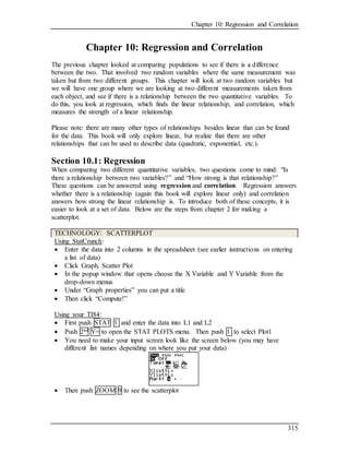
 Then push ZOOM 9 to see the scatterplot

316
Example #10.1.1: Making a Scatterplot
Is there a relationship between the alcohol content and the number of calories in
12-ounce beer? To determine if there is one, a random sample was taken of
beer’s alcohol content and calories ("Calories in beer," 2011), and the data are in
table #10.1.1. Make a scatterplot of the data.
Table #10.1.1: Alcohol and Calorie Content in Beer
Brand Brewery Alcohol Content Calories in 12 oz
Big Sky Scape Goat Pale Ale Big Sky Brewing 4.70% 163
Sierra Nevada Harvest Ale Sierra Nevada 6.70% 215
Steel Reserve MillerCoors 8.10% 222
O'Doul's Anheuser Busch 0.40% 70
Coors Light MillerCoors 4.15% 104
Genesee Cream Ale High Falls Brewing 5.10% 162
Sierra Nevada Summerfest Beer Sierra Nevada 5.00% 158
Michelob Beer Anheuser Busch 5.00% 155
Flying Dog Doggie Style Flying Dog Brewery 4.70% 158
Big Sky I.P.A. Big Sky Brewing 6.20% 195
Solution:
It is helpful to state the random variables in the context of the problem.
rv X = alcohol content in a randomly selected 12-ounce beer
rv Y = number of calories in that same randomly selected 12-ounce beer
Figure #10.1.1: Scatter Plot of BeerData
This scatter plot looks fairly linear. However, notice that there is one beer in the
list that is actually considered a non-alcoholic beer. That value is probably an
outlier since it is a non-alcoholic beer. The rest of the analysis will not include
O’Doul’s. You cannot just remove data points, but in this case, it makes more
sense to, since all the other beers have a fairly large alcohol content.
2 4 6 8
050100150200250
Calories vs Alcohol Content
Alcohol Content (%)
Caloriesin12inBeer

317
The scatterplot without O’Doul’s is as follows: (TI84 and StatCrunch graphs)
The relation looks fairly linear. The next step is to find a line that best fits the data and
the corresponding equation of that line.
In high school algebra you spent many, many months each year on linear functions. Most
of you are familiar with the equation Y = mX + b that is used in most algebra texts. Some
of the more current algebra textbooks use the equation Y = a + bX (this matches the
equation that the calculator uses and the linear equation we will use in this class).
 X is the independent variable and is also called the predictor variable
 Y is the dependent variable and is also called the response variable
 The coefficient of X is the slope and the constant term is the Y-intercept.
 In this course we are going to be using the equation 𝑌̂( 𝑥) = 𝑎 + 𝑏(𝑋)
 The “hat” on the Y reminds us that this is an estimated or predicted value of Y
 slope = coefficient of X = b =
𝑏
1
=
change in Y
change in X
which means for each 1 unit
increase in X, Y changes by b units on average. Whether Y increases or decreases
for every 1 unit increase in X depends on the sign of the slope.
 Y-intercept = (0, 𝑎) which means when X = 0, Y = 𝑎 (Sometimes the Y-intercept
will have no physical meaning with respect to the linear regression problem that
we are doing because it falls outside of the values that make sense or outside the
range of values sampled from, but it is still part of the equation and is needed to
plot the line)
 This equation should only be used for X-values between Xmin and Xmax. Many
relationships between variables may look linear in a particular range of X-values
but once you go beyond those values the relation may no longer be linear.
There are many conditions to check when doing linear regression. In this level of a
course, we are just going to look at checking the following assumptions:
1. The set (X,Y) of ordered pairs is a random sample from the population of all such
possible (X,Y) pairs.
2. The scatter plot of X versus Y has a roughly linear pattern with no outliers.
 We will get a hypothesis test in section 10.3 to tell us if what we see is linear
enough or not.

318
In graphing real-world data, the scatterplots do not look as perfect as the ones from
algebra. In this case we find what we call a best-fitting line using a process called
regression. The notation we use in this class for the equation of the best-fitting line (also
called the least-squares regression equation) is as follows:
𝑌̂( 𝑋) = 𝑎 + 𝑏(𝑋)
TECHNOLOGY: REGRESSION EQUATION, 𝑌̂( 𝑋) = 𝑎 + 𝑏(𝑋)
Using StatCrunch:
 Enter data into 2 columns in the spreadsheet (see earlier instructions on entering a
list of data)
 Click Stat, Regression, Simple Linear
drop-down menus
Using your TI84:
 Then push STAT ← to open the TESTS menu. Scroll down until you see
“LinRegTTest” and push ENTER. You can then enter the names of the lists where
you put your data.
 You also need to tell the TI to store this linear regression equation in Y1 by typing
VARS → 1 1 next to "RegEQ" on the LinRegTTest input screen.
 Your input screen should look like the one below (you may have stored your data
in different lists. For now, which inequality you highlight does not matter, but it
will in the later section when we do the hypothesis test).
 After you highlight “Calculate” and push ENTER you will get the following output
screen. You will need to scroll down to see all of the output.
 This equation is written as 𝑌̂( 𝑋) = 𝑎 + 𝑏(𝑋)
 slope =
𝑏
1
, which tells us on average how much we expect Y to change when X
increases by 1 unit
 Y-intercept: (0, 𝑎), which tells us the value of Y when X is 0. For many
applications, we do not interpret the Y-intercept because X = 0 is out of the scope
of the data and usually does not make sense to talk about (like a baby that weighs 0
pounds)

319
Example #10.1.2: Finding the Equation of the Line of Best Fit
Use the data from Example #10.1.1 (removing O’Doul’s) to do the following:
a) Find the equation of the line of best fit.
Solution:
Alcohol content is the explanatory variable and number of calories is the response
variable.
TI84: Values of alcohol content are in L1 and values of calories are in L2.
StatCrunch: Using Stat, Regression, Simple Linear
So the equation of the line of best fit is as follows:
𝑌̂( 𝑋) = 25.03123606+ 26.31860776(𝑋), where 4.15% ≤ 𝑋 ≤ 8.1%
b) Draw the scatterplot and the line of best fit on the same set of axes.
Solution:
Since we told the calculator to store the equation in Y1, if you push ZOOM 9 you
will see the scatterplot and the line of best fit drawn on the same set of axes. That
graph is also on the second page of results in StatCrunch.

320
c) Interpret the slope and Y-intercept in context.
Solution:
Slope =
change in Y
change in X
=
𝑐ℎ𝑎𝑛𝑔𝑒 𝑖𝑛 𝑐𝑎𝑙𝑜𝑟𝑖𝑒𝑠
𝑐ℎ𝑎𝑛𝑔𝑒 𝑖𝑛 𝑎𝑙𝑐𝑜ℎ𝑜𝑙 𝑐𝑜𝑛𝑡𝑒𝑛𝑡
≈
26.32 𝑐𝑎𝑙𝑜𝑟𝑖𝑒𝑠
1%
The slope here tells us that for every 1% increase in the alcohol content of beer
we expect the calories to increase by 26.32 on average.
The Y-intercept here would be (0%, 25.03 calories). This has no meaning with
respect to this problem since we only looked at alcoholic beers (so it makes no
sense to talk about a beer with 0% alcohol).
What makes this the best fitting line? The process of regression is used to find the line
that best fits the data. The criteria for the best fitting line that technology will use are as
follows.
1. The line must pass through the point (X̅,Y̅)
2. The line must make the sum of the square of the residuals as small as possible
What the heck is a residual? When you draw a line that “best” fits the data, that line will
not be able to pass through all of the points (in fact it might not pass through a single
point from the data). You can see that in the graph in Example #10.1.2. The residuals
give us a way to measure how far the line is vertically from each point in the data set.
Residual – the difference between the actual Y value and the predicted Y value on the
regression line for a particular value of X, 𝑥0. This is the directed vertical distance
between the actual point in the data and the corresponding point on the regression line.
residual = 𝑌( 𝑥0)− 𝑌̂(𝑥0)
 Data points above the line will have positive residuals.
 Data points below the line will have negative residuals.
 The sum of the residuals is always 0
The regression line and the residuals are displayed in figure #10.1.2.
Figure #10.1.2: Scatter Plot of BeerData with RegressionLine and Residuals

321
Example #10.1.3: Computing Predicted Values and Residuals.
a.) Use the regression equation to predict the number of calories when the alcohol
content is 6.50% based on the data given in Table #10.1.2 ("Calories in beer,"
2011) from a random sample of 9 beers.
Table #10.1.2: Alcohol and Calorie Content in Beerwithout Outlier
Brand Brewery Alcohol
Content
Calories
in 12 oz
Solution:
State random variables
rv Y = number of calories in that same randomly selected 12-ounce
beer
In this case, 𝑥0 = 6.50
First check that 6.50 is between Xmin and Xmax from the data.
4.15 ≤ 6.50 ≤ 8.1
𝑌̂(6.50) ≈ 25.03123606+ 26.31860776(6.50) ≈ 196.1 calories
This equation was also stored in Y1. So you can also find this predicted
value as follows:
𝑌̂(6.50) = 𝑌1(6.50) ≈ 196.1 calories
The following keypunches will type a Y1: VARS → 1 1
If you are drinking a beer that has 6.50% alcohol content, then it is predicted
to have 196.1 calories. Notice, the mean number of calories of the sample of
9 beers is about 170.2 calories. The value of 196.1 seems like a better
estimate than the mean when looking at the original data. The regression
equation is a better estimate than just the mean, since the regression equation
takes into account the alcohol content.
b.) Use the regression equation to predict the number of calories when the alcohol
content is 2.00%.

322
Solution:
First check that 2.00 is between Xmin and Xmax from the data.
2.00 is not between 4.15 and 8.1
The equation should not be used to predict that calories for this beer. We also
should not use the mean from the sample of 12 beers either since there were
no beers in the sample with an alcohol content as low as 2.00%.
c.) Find the residual associated with the beer that had 6.70% alcohol.
Solution:
residual = 𝑌( 𝑥0)− 𝑌̂(𝑥0) = actual Y – predicted Y
residual = 𝑌(6.70)− 𝑌̂(6.70) = actual Y – predicted Y
To get 𝑌(6.70) you need to look in the data table. This beer is highlighted in
Table #10.1.2. This beer has 215 calories. So 𝑌(6.70) = 215
To get 𝑌̂(6.70) you need to use the equation.
𝑌̂(6.70) ≈ 25.03123606+ 26.31860776(6.70) ≈ 201.4 calories
This beer with 6.70% alcohol actually had 215 calories but the linear model
predicted that it would have 201.4 calories.
residual = 𝑌(6.70)− 𝑌̂(6.70)≈ 215 calories − 201.4 calories ≈
13.6 calories
This residual means that the actual value was about 13.6 calories above the
predicted value.
Example #10.1.4: Interpreting a Negative Slope
For a set of sample data of elevation (in ft) and high temperature (in ℉) for
randomly selected cities, the following equation of the least squares regression
line was computed. Interpret the slope in context.
𝑌̂( 𝑥) ≈ 77.37 − 0.0039(𝑋), 3000 ≤ 𝑋 ≤ 7000
Solution:
Slope =
change in Y
change in X
=
𝑐ℎ𝑎𝑛𝑔𝑒 𝑖𝑛 ℎ𝑖𝑔ℎ 𝑡𝑒𝑚𝑝𝑒𝑟𝑎𝑡𝑢𝑟𝑒
𝑐ℎ𝑎𝑛𝑔𝑒 𝑖𝑛 𝑒𝑙𝑒𝑣𝑎𝑡𝑖𝑜𝑛
≈
−0.0039 ℉
1 𝑓𝑡
The slope here tells us that for every 1 foot increase in elevation we expect the
high temperature to decrease by 0.0039 ℉ on average. (NOTE: The word
“decrease” takes care of the negative sign in the numeric value of the slope.)

323
Section10.1: Homework
1.) When an anthropologist finds skeletal remains, they need to figure out the height
of the person. The height of a person (in cm) and the length of their metacarpal
bone 1 (in cm) were collected and are in table #10.1.5 ("Prediction of height,"
2013).
Table #10.1.5: Data of Metacarpal versus Height
Length of
Metacarpal
(cm)
Height of
Person
(cm)
45 171
51 178
39 157
41 163
48 172
49 183
46 173
43 175
47 173
a) State the random variables.
b) Make a scatterplot of X versus Y.
c) Find the equation of the best-fitting line (the least squares regression
equation).
d) Interpret the slope in the context of this problem.
e) Interpret the Y-intercept in the context of this problem or state why it does not
make sense to do so.
f) Predict the height of a person for a metacarpal length of 44 cm or state why
you shouldn’t.
g) Predict the height of a person for a metacarpal length of 55 cm or state why
you shouldn’t.
h) Compute the residual for the person with a metacarpal length of 45 cm.
Interpret what this value means in the context of this problem.

324
2.) Table #10.1.6 contains the value of the house and the amount of annual rental
income in a year that the house brings in ("Capital and rental," 2013).
Table #10.1.6: Data of House Value versus Annual Rental Income
Value Rental Value Rental Value Rental Value Rental
81000 6656 77000 4576 75000 7280 67500 6864
95000 7904 94000 8736 90000 6240 85000 7072
121000 12064 115000 7904 110000 7072 104000 7904
135000 8320 130000 9776 126000 6240 125000 7904
145000 8320 140000 9568 140000 9152 135000 7488
165000 13312 165000 8528 155000 7488 148000 8320
178000 11856 174000 10400 170000 9568 170000 12688
200000 12272 200000 10608 194000 11232 190000 8320
214000 8528 208000 10400 200000 10400 200000 8320
240000 10192 240000 12064 240000 11648 225000 12480
289000 11648 270000 12896 262000 10192 244500 11232
325000 12480 310000 12480 303000 12272 300000 12480
equation).
f) Predict the rental income a house worth $230,000 or state why you shouldn’t.
g) Predict the rental income a house worth $400,000 or state why you shouldn’t.
h) Compute the residual for the house worth $214,000. Interpret what this value
means in the context of this problem.

325
3.) The World Bank collects information on the life expectancy of a person in each
country ("Life expectancy at," 2013) and the fertility rate (average number of
children per woman) in the country ("Fertility rate," 2013). The data for 24
randomly selected countries for the year 2011 are in table #10.1.7.
Table #10.1.7: Data of Fertility Rates versus Life Expectancy
Fertility
Rate
Life
Expectancy
1.7 77.2
5.8 55.4
2.2 69.9
2.1 76.4
1.8 75.0
2.0 78.2
2.6 73.0
2.8 70.8
1.4 82.6
2.6 68.9
1.5 81.0
6.9 54.2
2.4 67.1
1.5 73.3
2.5 74.2
1.4 80.7
2.9 72.1
2.1 78.3
4.7 62.9
6.8 54.4
5.2 55.9
4.2 66.0
1.5 76.0
3.9 72.3
equation).
f) Predict the life expectancy of a country that has a fertility rate of 2.7 or state
why you shouldn’t.
g) Predict the life expectancy of a country that has a fertility rate of 8.1 or state
h) Compute the residual for the country with a fertility rate of 5.8. Interpret what
this value means in the context of this problem.

326
4.) The height and weight of baseball players are in table #10.1.9 ("MLB heights
weights," 2013).
Table #10.1.9: Heights and Weights of Baseball Players
Height
(inches)
Weight
(pounds)
76 212
76 224
72 180
74 210
75 215
71 200
77 235
78 235
77 194
76 185
72 180
72 170
75 220
74 228
73 210
72 180
70 185
73 190
71 186
74 200
74 200
75 210
78 240
72 208
75 180
equation).
f) Predict the weight of a baseball player that is 75 inches tall or state why you
shouldn’t.
g) Predict the weight of a baseball player that is 68 inches tall or state why you
shouldn’t.
h) Compute the residual for the baseball player that is 76 inches tall and weighs
212 pounds. Interpret what this value means in the context of this problem.

327
5.) A random sample of beef hotdogs was taken and the amount of sodium (in mg)
and calories were measured. ("Data hotdogs," 2013) The data are in table
#10.1.11.
Table #10.1.11: Calories and Sodium Levels in Beef Hotdogs
Calories Sodium
186 495
181 477
176 425
149 322
184 482
190 587
158 370
139 322
175 479
148 375
152 330
111 300
141 386
153 401
190 645
157 440
131 317
149 319
135 298
132 253
equation).
f) Predict the amount of sodium a beef hotdog has if it has 170 calories or state
g) Predict the amount of sodium a beef hotdog has if it has 120 calories or state
h) Compute the residual for the beef hotdog with 153 calories. Interpret what
this value means in the context of this problem.

328
6.) Per capita income in 1960 dollars for European countries and the percent of the
labor force that works in agriculture in 1960 are in table #10.1.12 ("OECD
economic development," 2013).
Table #10.1.12: Percent of Labor in Agriculture and Per Capita Income for
European Countries
Country Percent in
Agriculture
Per capita
income
Sweden 14 1644
Switzerland 11 1361
Luxembourg 15 1242
U. Kingdom 4 1105
Denmark 18 1049
W. Germany 15 1035
France 20 1013
Belgium 6 1005
Norway 20 977
Iceland 25 839
Netherlands 11 810
Austria 23 681
Ireland 36 529
Italy 27 504
Greece 56 324
Spain 42 290
Portugal 44 238
Turkey 79 177
equation).
f) Predict the per capita income in a country that has 21 percent of labor in
agriculture or state why you shouldn’t.
g) Predict the per capita income in a country that has 2 percent of labor in
agriculture or state why you shouldn’t.
h) Compute the residual for the country with 6 percent of labor in agriculture.
Interpret what this value means in the context of this problem.

329
7.) Cigarette smoking and cancer have been linked. The number of deaths per one
hundred thousand from bladder cancer and the number of cigarettes sold per
capita in 1960 are in table #10.1.13 ("Smoking and cancer," 2013) for 44
randomly selected countries. Create a scatter plot and find a regression equation
between cigarette smoking and deaths of bladder cancer. Then use the regression
equation to find the number of deaths from bladder cancer when the cigarette
sales were 20 per capita and when the cigarette sales were 6 per capita. Which
number of deaths that you calculated do you think is closer to the true number?
Why?
Table #10.1.13: Number of Cigarettes and Number of Bladder Cancer
Deaths in 1960
Cigarette
Sales (per
Capita)
Bladder
Cancer
Deaths (per
100
Thousand)
Cigarette
Sales (per
Capita)
Bladder
Cancer
Deaths (per
100
Thousand)
Cigarette
Sales (per
Capita)
Bladder
Cancer
Deaths (per
100
Thousand)
18.20 2.90 42.40 6.54 28.92 4.79
25.82 3.52 28.64 5.98 25.91 5.21
18.24 2.99 21.16 2.90 26.92 4.69
28.60 4.46 29.14 5.30 24.96 5.27
31.10 5.11 19.96 2.89 22.06 3.72
33.60 4.78 26.38 4.47 16.08 3.06
40.46 5.60 23.44 2.93 27.56 4.04
28.27 4.46 23.78 4.89 21.17 4.04
20.10 3.08 29.18 4.99 21.25 5.14
27.91 4.75 18.06 3.25 22.86 4.78
26.18 4.09 20.94 3.64 28.04 3.20
22.12 4.23 20.08 2.94 30.34 3.46
21.84 2.91 22.57 3.21 23.75 3.95
23.44 2.86 14.00 3.31 23.32 3.72
21.58 4.65 25.89 4.63
equation).
f) Predict the number of deaths from bladder cancer when the cigarette sales
were 20 per capita or state why you shouldn’t.
g) Predict the number of deaths from bladder cancer when the cigarette sales
were 6 per capita or state why you shouldn’t.
h) Compute the residual for the country where cigarette sales were 18.20 per
capita. Interpret what this value means in the context of this problem.

330
8.) The weight of a car can influence the mileage that the car can obtain. A random
sample of cars’ weights and mileage was collected and are in table #10.1.14
("Passenger car mileage," 2013). Create a scatter plot and find a regression
equation between weight of cars and mileage. Then use the regression equation to
find the mileage on a car that weighs 3800 pounds and on a car that weighs 2000
pounds. Which mileage that you calculated do you think is closer to the true
mileage? Why?
Table #10.1.14: Weights and Mileages of Cars
Weight (100 pounds) Mileage (mpg) Weight (100 pounds) Mileage (mpg)
22.5 53.3 35.0 31.3
22.5 41.1 35.0 28.0
22.5 38.9 35.0 28.0
25.0 40.9 35.0 28.0
27.5 46.9 40.0 23.6
27.5 36.3 40.0 23.6
30.0 32.2 40.0 23.4
30.0 32.2 40.0 23.1
30.0 31.5 45.0 19.5
30.0 31.4 45.0 17.2
30.0 31.4 45.0 17.0
35.0 32.6 55.0 13.2
35.0 31.3
equation).
f) Predict the mileage on a car that weighs 3800 pounds or state why you
shouldn’t.
g) Predict the mileage on a car that weighs 2000 pounds or state why you
shouldn’t.
h) Compute the residual for the car that weighs 55.0 pounds. Interpret what this
value means in the context of this problem.

331
Section 10.2: Correlation
A correlation exists between two quantitative variables when the values of one
quantitative variable are somehow associated with the values of the other quantitative
variable.
When you see a pattern in the data you say there is a correlation in the data. Though this
book is only dealing with linear patterns, patterns can be other math models such as
exponential, logarithmic, or periodic. To see this pattern, you can draw a scatter plot of
the data.
Remember to read graphs from left to right, the same as you read words. If the graph
goes up the correlation is positive and if the graph goes down the correlation is negative.
The words “weak”, “moderate”, and “strong” are used to describe the strength of the
relationship between the two variables.
Figure 10.2.1: Correlation Graphs
We need a numeric way to measure the strength of the linear relation between two
variables. This measure needs to be unitless. If someone measures heights in inches and
weights in pounds and someone else takes the same group of people and measures
heights in centimeters and weights in kilograms, then whatever we use to measure the
strength of the relationship between height and weight should be the same. The strength
should not depend on the units of measurement. What statistic do we have that is
unitless?......z-scores.

332
The formula below is what was developed by Karl Pearson to measure the strength of
linear relation between two quantitative variables. If we had to make these computations
by hand (which we don’t!) we would first need to convert all of the X-coordinates into
their corresponding z-scores and then the same for the Y-coordinates. We will be using
technology to compute this.
𝑟 =
∑ 𝑧 𝑥 ∙ 𝑧 𝑦
𝑛 − 1
Linear correlation coefficient – is a number that describes the strength of the linear
relationship between the two variables. It is also called the Pearson correlation
coefficient after Karl Pearson who developed it. The symbol for the sample linear
correlation coefficient is r. The symbol for the population correlation coefficient is r
(Greek letter rho)
r is always between -1 and 1, inclusive.
r = -1 means there is a perfect negative linear correlation
r = 1 means there is a perfect positive linear correlation.
The closer r is to 1 or -1, the stronger the linear correlation.
The closer r is to 0, the weaker the linear correlation.
BE CAREFUL: r = 0 does not mean there is no correlation. It just means there is no
linear correlation. There might be a very strong curved pattern like in the last graph on
the previous page.
There are many conditions to check for linear correlation. In this level of a course, we
are just going to look at checking the following assumptions (these are the same
assumptions we had in the last section for regression):
1. The set (X,Y) of ordered pairs is a random sample from the population of all such
possible (X,Y) pairs.
2. The scatter plot of X versus Y has a roughly linear pattern with no outliers.
 We will get a hypothesis test in section 10.3 to tell us if what we see is linear
enough or not.
The value of the sample linear correlation coefficient is on the same output screen that
was used in the last section to get the equation of the best-fitting line.
This sample linear correlation coefficient is computed from unitless z-scores, so it is
unitless.

333
TECHNOLOGY: LINEAR CORRELATION COEFFICIENT
Using StatCrunch:
 Enter data into 2 columns in the spreadsheet (see earlier instructions on entering a
list of data)
 Click Stat, Regression, Simple Linear
drop-down menus
Using your TI84:
 Then push STAT ← to open the TESTS menu. Scroll down until you see
“LinRegTTest” and push ENTER. You can then enter the names of the lists where
you put your data.
 Your input screen should look like the one below (you may have stored your data
in different lists. For now, which inequality you highlight does not matter, but it
will in the later section when we do the hypothesis test).
 After you highlight “Calculate” and push ENTER you will get the following output
screen. You will need to scroll down to see all of the output.
 You will need to scroll down to the bottom of the output screens to see the value of
r.

334
Example #10.2.1: Calculating the Linear Correlation Coefficient, r
How strong is the positive relationship between the alcohol content and the
number of calories in 12-ounce beer? To determine if there is a positive linear
correlation, a random sample was taken of beer’s alcohol content and calories for
several different beers ("Calories in beer," 2011), and the data are in table #10.2.1.
Find the correlation coefficient and interpret that value.
Table #10.2.1: Alcohol and Calorie Content in Beerwithout Outlier
Brand Brewery Alcohol
Content
Calories
in 12 oz
Solution:
State random variables
rv Y = number of calories in that same randomly selected 12-ounce beer
Assumptions check:
1. The problem states that a random sample of beers was taken
2. The scatterplot of the data looked roughly linear with no outliers
TI84: Use the LinRegTTest in the STAT menu. The setup is in figure 10.2.2.
Figure #10.2.2: Setup for Linear RegressionTest on TI-84

335
Figure #10.2.3: Results for Linear RegressionTest on TI-84
StatCrunch: Using Stat, Regression, Simple Linear
The correlation coefficient is 𝑟 ≈ 0.913. This is close to 1, so it looks like there
is a strong, positive linear correlation between alcohol content and number of
calories for beer.
Causation
One common mistake people make is to assume that because there is a correlation, then
one variable causes the other. This is usually not the case. That would be like saying the
amount of alcohol in the beer causes it to have a certain number of calories. However,
fermentation of sugars is what causes the alcohol content. The more sugars you have, the
more alcohol can be made, and the more sugar, the higher the calories. It is actually the
amount of sugar that causes both. Do not confuse the idea of correlation with the concept
of causation. Just because two variables are correlated does not mean one causes the
other to happen.
Example #10.2.2: Correlation Versus Causation
A study showed a strong linear correlation between per capita beer consumption and
teacher’s salaries. Does giving a teacher a raise cause people to buy more beer?
Does buying more beer cause teachers to get a raise?
Solution:
There is probably some other factor causing both of them to increase at the same
time. Think about this: In a town where people have little extra money, they won’t
have money for beer and they won’t give teachers raises. In another town where
people have more extra money to spend it will be easier for them to buy more beer
and they would be more willing to give teachers raises.
Remember a correlation only means a pattern exists. It does not mean that one variable
causes the other variable to change. Correlation does not imply causation.

336
Explained Variation
As stated before, there is some variability in the dependent variable values, such as
calories. Some of the variation in calories is due to alcohol content and some is due to
other factors. How much of the variation in the calories is due to alcohol content?
You can have two beers at the same alcohol content, but beer one has higher calories
because of the other ingredients. Some variability is explained by the model and some
variability is not explained. The coefficient of determination gives us the proportion of
the variation in Y that is explained by the model with X as its predictor variable.
Coefficient of determination – measures the proportion of the variability in Y that is
explained by the linear model with X as its predictor variable.
 This value is next to r2 on the LinRegTTest output screen
 This proportion is often changed to a percentage when its value is interpreted.
Example #10.2.3: Finding the Coefficient of Determination
Find the coefficient of determination for the beer data in Example 10.2.1 and
interpret the value.
Solution:
From the calculator results,
𝑟2
≈ 0.834
Interpret:
Thus, about 83.4% of the variation in calories is explained by the linear
relationship between alcohol content and calories. The other 16.6% of the
variation in calories is due to other factors.
Now that you have a correlation coefficient for the sample data, how can you tell if it is
significant or not to determine if this linear relation exists for the population of objects?
This will be answered in the next section.

337
Section10.2:Homework
These problems use the same data as section 10.1.
bone 1 (in cm) were collected and are in table #10.1.5 ("Prediction of height,"
2013). Find the correlation coefficient and coefficient of determination and then
interpret both.
2.) Table #10.1.6 contains the value of the house and the amount of rental income in
a year that the house brings in ("Capital and rental," 2013). Find the correlation
coefficient and coefficient of determination and then interpret both.
country ("Life expectancy at," 2013) and the fertility rate per woman in the
country ("Fertility rate," 2013). The data for 24 randomly selected countries for
the year 2011 are in table #10.1.7. Find the correlation coefficient and coefficient
of determination and then interpret both.
4.) The height and weight of baseball players are in table #10.1.9 ("MLB
heightsweights," 2013). Find the correlation coefficient and coefficient of
determination and then interpret both.
#10.1.11. Find the correlation coefficient and coefficient of determination
and then interpret both.
economic development," 2013). Find the correlation coefficient and coefficient
of determination and then interpret both.
capita in 1960 are in table #10.1.13 ("Smoking and cancer," 2013). Find the
correlation coefficient and coefficient of determination and then interpret
both.
sample of cars weights and mileage was collected and are in table #10.1.14
("Passenger car mileage," 2013). Find the correlation coefficient and
coefficient of determination and then interpret both.

338
9.) There is a negative correlation between police expenditure and crime rate. Does
this mean that spending more money on police causes the crime rate to decrease?
Explain your answer.
10.) There is a positive correlation between tobacco sales and alcohol sales. Does that
mean that using tobacco causes a person to also drink alcohol? Explain your
answer.
11.) There is a positive correlation between the average temperature in a location and
the morality rate from breast cancer. Does that mean that higher temperatures
cause more women to die of breast cancer? Explain your answer.
12.) There is a positive correlation between the length of time a tableware company
polishes a dish and the price of the dish. Does that mean that the time a plate is
polished determines the price of the dish? Explain your answer.
Section 10.3: Inference for Regression and Correlation
In the last section we computed the sample linear correlation coefficient. How do we
know if there is enough evidence in the sample data to conclude that a linear relation
exists in the population? We perform a hypothesis test. In this case the parameter we
will be testing is rho, 𝜌, which is the population linear correlation coefficient.

339
Hypothesis Test for Population Correlation (Lin Reg T-Test)
1. State the random variable and the Parameter in words.
𝜌 = the linear correlation between __ and __ for all _____
rv 𝑟 = the linear correlation between __ and __ for __ r.s. _______
2. State the null and alternative Hypotheses and the level of significance
TWO-TAILED TEST LEFT-TAILED TEST RIGHT-TAILED TEST
𝐻0: 𝜌 = 0
𝐻𝐴: 𝜌 ≠ 0 this tests for any
kind of a linear relation
𝐻0: 𝜌 = 0
𝐻𝐴: 𝜌 < 0 this tests for a
negative linear relation
𝐻0: 𝜌 = 0
𝐻𝐴: 𝜌 > 0 this tests for a
positive linear relation
Also, state your 𝛼 level here.
3. State and check the Assumptions for a hypothesis test
a) The set (X,Y) of ordered pairs is a random sample from the population of
all such possible (X,Y) pairs.
b) The scatter plot of x versus y has a roughly linear pattern with no outliers.
4. Name the hypothesis test used
In this case the assumptions for the Lin Reg T-Test have been satisfied.
5. Find the sample statistic and Test statistic
Sample correlation coefficient:
𝑟 = value next to r on the output screen
Test Statistic:
t =
r
1- r2
n - 2
6. Obtain the p-value and illustrate the meaning of the p-value, sample
statistic and test statistic
𝑟: 0
t: 0
𝑟: 0
t: 0
𝑟: 0
t: 0
7. Make a decision about H0
Reject 𝐻0 if the p-value ≤ a and fail to reject 𝐻0 if the p-value > a
8. State a conclusion in the context of the problem
 If you reject 𝐻0, then there is significant evidence to conclude (𝐻𝐴 in
context)
 If you fail to reject 𝐻0, then there is NOT significant evidence to conclude
(𝐻𝐴 in context)
 We never say “accept 𝐻0”

340
Example #10.3.1: Testing the Claim of a Linear Correlation
Is there a positive linear correlation between beer’s alcohol content and calories?
To determine if there is a positive linear correlation, a random sample was taken
of beer’s alcohol content and calories for several different beers ("Calories in
beer,," 2011), and the data is in table #10.2.1. Test at the 5% level.
Solution:
1. State the random variable and the Parameter in words.
𝜌 = the linear correlation between alcohol content and number of calories for
all beers with an alcohol content between 4.15% and 8.1 %
rv 𝑟 = the linear correlation between alcohol content and number of calories
for 9 randomly selected beers with an alcohol content between 4.15% and
8.1 %
2. State the null and alternative Hypotheses and the level of significance
Since you are asked if there is a positive correlation, use r > 0.
𝐻0: 𝜌 = 0
𝐻𝐴: 𝜌 > 0
a = 0.05
3. State and check the Assumptions for the hypothesis test
1. The problem states that a random sample of 9 beers was taken
2. The scatterplot of the data looked roughly linear with no outliers
4. Name the hypothesis test used
In this case the assumptions for the Linear Regression T-Test have been met.
5. Find the sample statistic and Test statistic
TI84: Use LinRegTTest from STAT TESTS
Input screen:
Output screen:

341
StatCrunch: Use Stat, Regression, Simple Linear
We need the T-Stat and P-value in the “Slope” row
Sample correlation coefficient:
𝑟 ≈ 0.913
Test Statistic: 𝑡 =
𝑟
√
1−𝑟2
𝑛−2
=
0.9134413647
√
1−0.8343751268
9−2
≈ 5.94
This means the value of r is about 5.94 standard deviations above the
hypothesized value in the null hypothesis.
6. Obtain the p-value and illustrate the meaning of the p-value, sample statistic
and test statistic.
p-value ≈ 2.884 × 10−4
≈ 0.0003
7. Make a decision about 𝐻0
Since the p-value ≤ 0.05, reject 𝐻0
8. State a conclusion in the context of the problem
There is enough evidence to show that there is a positive correlation between
alcohol content and number of calories in all 12-ounce bottles of beer with
alcohol content between 4.15% and 8.1%.

342
Section10.3:Homework
For each problem, use the PHANTOMS process.
bone one (in cm) were collected and are in table #10.1.5 ("Prediction of height,"
2013). Test at the 1% level for a positive correlation between length of
metacarpal bone one and height of a person.
2.) Table #10.1.6 contains the value of the house and the amount of rental income in
a year that the house brings in ("Capital and rental," 2013). Test at the 5% level
for a positive correlation between house value and annual rental amount.
country ("Life expectancy at," 2013) and the fertility rate per woman in the
country ("Fertility rate," 2013). The data for 24 randomly selected countries for
the year 2011 are in table #10.1.7. Test at the 1% level for a negative correlation
between fertility rate and life expectancy.
4.) The height and weight of baseball players are in table #10.1.9 ("MLB heights
weights," 2013). Test at the 5% level for a positive correlation between
height and weight of baseball players.
#10.1.11. Test at the 5% level for a positive correlation between number of
calories and amount of sodium.
economic development," 2013). Test at the 5% level for a negative correlation
between percent of labor force in agriculture and per capita income.
capita in 1960 are in table #10.1.13 ("Smoking and cancer," 2013). Test at the
1% level for a positive correlation between cigarette smoking and deaths of
bladder cancer.
sample of cars weights and mileage was collected and are in table #10.1.14
("Passenger car mileage," 2013). Test at the 5% level for a negative
correlation between the weight of cars and mileage.

343
Data Source:
Brain2bodyweight. (2013, November 16). Retrieved from
http://wiki.stat.ucla.edu/socr/index.php/SOCR_Data_Brain2BodyWeight
Calories in beer, beer alcohol, beer carbohydrates. (2011, October 25). Retrieved from
www.beer100.com/beercalories.htm
Capital and rental values of Auckland properties. (2013, September 26). Retrieved from
http://www.statsci.org/data/oz/rentcap.html
Data hotdogs. (2013, November 16). Retrieved from
http://wiki.stat.ucla.edu/socr/index.php/SOCR_012708_ID_Data_HotDogs
Fertility rate. (2013, October 14). Retrieved from
http://data.worldbank.org/indicator/SP.DYN.TFRT.IN
Health expenditure. (2013, October 14). Retrieved from
http://data.worldbank.org/indicator/SH.XPD.TOTL.ZS
Life expectancy at birth. (2013, October 14). Retrieved from
http://data.worldbank.org/indicator/SP.DYN.LE00.IN
MLB heightsweights. (2013, November 16). Retrieved from
http://wiki.stat.ucla.edu/socr/index.php/SOCR_Data_MLB_HeightsWeights
OECD economic development. (2013, December 04). Retrieved from
http://lib.stat.cmu.edu/DASL/Datafiles/oecdat.html
Passenger car mileage. (2013, December 04). Retrieved from
http://lib.stat.cmu.edu/DASL/Datafiles/carmpgdat.html
Prediction of height from metacarpal bone length. (2013, September 26). Retrieved from
http://www.statsci.org/data/general/stature.html
Pregnant woman receiving prenatal care. (2013, October 14). Retrieved from
http://data.worldbank.org/indicator/SH.STA.ANVC.ZS
Smoking and cancer. (2013, December 04). Retrieved from
http://lib.stat.cmu.edu/DASL/Datafiles/cigcancerdat.html

Chapter 10

Recommended

Recommended

More Related Content

What's hot

What's hot (20)

Similar to Chapter 10

Similar to Chapter 10 (20)

More from MaryWall14

More from MaryWall14 (20)

Recently uploaded

Recently uploaded (20)

Chapter 10