This document provides instructions for analyzing education test score data from 200 students using SPSS. It includes questions to guide analysis of relationships between test scores (dependent variable) and demographic factors like gender, race, and school type (independent variables). Students are asked to identify variables of interest, run assumption tests, conduct a one-way ANOVA and post hoc tests to address a hypothesis, and interpret the results.

1. For this assignment, use the aschooltest.sav dataset.
The dataset consists of Reading, Writing, Math, Science, and
Social Studies test scores for 200 students. Demographic data
include gender, race, SES, school type, and program type.
Instructions:
Work with the aschooltest.sav datafile and respond to the
following questions in a few sentences. Please submit your
SPSS output either in your assignment or separately.
1. Identify an Independent and Dependent Variable (of your
choice) and develop a hypothesis about what you expect to find.
(
note: the IV is a grouping variable, which means it
needs to have more than 2 categories and the DV is continuous)
2. Run Assumption tests for Normality and initial Homogeneity
of Variance. What are your results?
3. Run the one-way ANOVA with the Levene test & Tukey post
hoc test.
a. What are the results of the Levene test? What does this mean?
b. What are the results of the one-way ANOVA (use notation)?
What does it mean?
c. Are post hoc tests necessary? If so, what are the results of
those analyses?

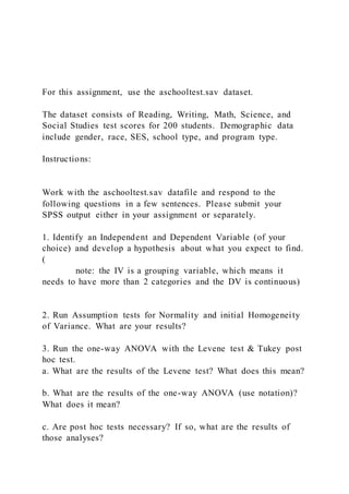
2. 4. How do your analyses address your hypotheses?
Is concentration of single parent families associated with
reading scores?
Using the AECF state data, the regression below measures the
effect of the state's percentage of single parent families on the
percentage of 4th graders with below basic reading scores.
%belowbasicread = β0 + β1x%SPF + u
Stata Output
1) Please write out the regression equation using the
coefficients in the table
2) Please provide an interpretation of the coefficient for SPF
3) How does the model fit?
4) What is the NULL hypothesis for a T test about a regression
coefficient?
5) What is the ALTERNATE hypothesis for a T test about a
regression coefficient?
6) Look at the p value for the coefficient SPF.
a) Report the p value
b) How many stars would it get if we used our standard
convention?
* p ≤ .1 ** p ≤ .05 *** p ≤ .01
image1.png
Two-Variable (Bivariate) Regression

3. In the last unit, we covered scatterplots and correlation. Social
scientists use these as descriptive tools for getting an idea about
how our variables of interest are related. But these tools only
get us so far. Regression analysis is the next step. Regression is
by far the most used tool in social science research.
Simple regression analysis can tell us several things:
1. Regression can estimate the relationship between x and y in
their
original units of measurement. To see why this is so
useful, consider the example of infant mortality and median
family income. Let’s say that a policymaker is interested in
knowing how much of a change in median family income is
needed to significantly reduce the infant mortality rate.
Correlation cannot answer this question, but regression can.
2. Regression can tell us how well the independent variable (x)
explains the dependent variable (y). The measure is called the
R square.
Simple Two-Variable (Bivariate) Regression
Regression uses the equation of a line to estimate the
relationship between x and y. You may remember back in
algebra learning about the equation of a line. Some learned it as
Y =s X + K or Y = mX + B. In statistics, we use a different
form:
Equation 1: Y = B0 + B1X + u
Let’s define each term in the equation:
· Y is the dependent variable. It is placed on the Y (vertical)
axis. In the example below, the dependent variable (Y) is the
infant mortality rate.
· B0 is the Y intercept. B0 is also referred to as “the constant.”
B0 is the point where the regression line crosses the Y axis.
Importantly, B0 is equal to the
predicted value of Ywhen X=0. In most cases, B0 is
does not get much attention for two reasons. First, the
researcher is usually interested in the relationship between x

4. and y. not the relationship between x and y at the single value
of x=0. Second, often independent variables do not take on the
value zero. Consider the AECF sample data. There are no states
with low-birth-weight percentages equal to zero, so we would
be extrapolating beyond what the data tell us.
· B1 is usually the main point of interest for researchers. It is
the slope of the line relating x to y. Researchers usually refer to
B1 as a slope coefficient, regression coefficient or simply a
coefficient.
B1 measures the change in Y for a one-unit change in x.
We represent change by the symbol ∆.
B1 =
· u is the error term. The error term is the distance between the
regression line and the dots on the scatterplot. Think about it,
regression estimates a single line through the cloud of data.
Naturally, the line does not hit all the data points. The degree to
which the line “misses” the data point is the error. u can also be
thought of as
all the other factors that affect the infant mortality rate
besides X. Importantly, we
assume that u is totally random given X.
The Black Box of Regression
Intuitively, regression analysis finds the line that is the best
predictor of the dependent variable. In the scatterplot, this line
is the one that “fits” the data the best. From the scatterplot, we
can see that the line does not go through all of the points in the
scatterplot. So, how does regression find this line? Regression
does this by finding the line that
minimizes the squared error. This is why regression is
also called “least squares” regression, because it minimizes the
squared error. The mathematical proof of this is not important,
if we understand that the regression line is the best fit for the
data.

5. The Predicted Value of Y, “yhat”
This is the estimated regression equation for the line that relates
infant mortality to low birth weight. Notice that this equation
does not contain an error term.
This makes sense, because this is the equation for the
regression line itself, not the actual data points (Y).
To make this distinction clear, define the term
Ŷ as the predicted values of Y along the regression line.
Ŷ is the predicted value of Y.
Equation 2: Ŷ = B0 + B1X
Subtracting the two gives:
Y = B0 + B1X + u
minus Ŷ = B0 + B1X
Y- Ŷ = u
This means each observation has values for Y, Ŷ and u. To
make this more concrete, let’s consider the example of infant
mortality and low birth weights.
Example: Infant Mortality and Low Birth Weights
For regression (unlike correlation), the researcher must specify
the dependent variable and the independent variable. Logically,
low birth weights should contribute to the infant mortality rate.
This makes sense too if we think about how the regression
equation works. To make things concrete, let’s say that a
lawmaker wants to know what effect low birth weights have on
infant mortality. The regression equation would be:
imr = B0 + B1lobweight + u
The Stata output has a lot of numbers. First let’s focus on
getting the actual estimates from the regression equation. We
get these numbers from the “coefficient column.
The bottom coefficient is labeled _cons. This is short for
“constant,” which is just another name for the y intercept, B0.
In this case, B0 = 1.205.
The coefficient labeled lobweight is the one we are really

6. interested in. This coefficient is B1. For this regression
B1=0.562.
Now we can write out the regression:
imr = B0 + B1lobweight + u
Substituting the numbers from the table:
imr = 1.205 + 0.562 lobweight + u
Interpreting the equation
B0 is usually not of interest to the researcher for reasons
discussed above.
B1 is the main coefficient of interest, especially for policy. It
tells us about the relationship between low birth weights and the
infant mortality rate.
Rules for Interpreting B1
· B1 measures the change in Y that results from a one unit
change in X.
· So, we can say that
a one unit change in X results in a B1 change in Y.
· In the regression above B1=0.562. That means that a one unit
change in percentage low birth weights results in a 0.562
change in the infant mortality rate.
The user-written Stata command aaplot. Gives a nice summary:
Model Fit
We already saw with scatterplots and correlation that different
models have different degree of “fit”, meaning how well the
data cluster around a line.
In regression, most analysts use the R Squared. The R Squared
has a ready interpretation once we know its properties:
Box 1: R Squared Properties
R2 Property 1: R square measures the proportion of the
variation in Y that is explained by the variation in X. An easier
way to say it is that the model explains (R2*100)%. For the
running example, the R2=0.436. That means that low brth
weights explain 43.6% of the variation in the infant mortality
rate. Or, for shrt, the model explains 43.6%.

7. R2 Property 2: R square will always (except in extreme and
unusual cases) lie somewhere on the interval between 0 and +1.
In other words, R squared will be a positive value between 0
and 1.
R2 Property 3: R squared values are only comparable
if the dependent variable is the same.This means that if
we want to compare two models on the R squared, Y must be
the same for both models.
Effect Size for R Squared
As with correlation coefficients, it is helpful to have a
benchmark to determine effect size. Recall that effect size tells
us how large (or small) the effect of one variable is on another.
We can use the benchmarks for r and square then to get the
benchmarks for R2.
Table 1: Cohen’s Effect Size Benchmarks for R Squared
R Squared
Effect Size
0.01 to 0.09
Small
0.09 to 0.25
Medium
0.25 to 1.0
Large
In the example, the R squared was 0.436, which exceeds 0.25,
so we conclude that the R squared shows a large effect size
between low birth weights and infant mortality.
Hypothesis Testing
So far, we have been focusing on how to interpret regression
results. But our results are derived from a
sample. This means we cannot be sure that our results
reflect what is going on in the population. Of course, we cannot
know what we don’t know, so instead we can do hypothesis
testing.

8. Generally, with hypothesis testing, we are focused on a “null”
hypothesis. This involves a little thought experiment. We ask
the following, “If there was no effect of X on Y in the
population, how likely is it that we would have obtained our
regression results?”
We write the null hypothesis as:
Null Hypothesis Ho: B1pop = 0
This is equivalent to saying that B1 in the population.
Remember, we do not know what B1 is in the population, we are
just testing if it is zero.
Alternative Hypothesis H1: B1pop ≠ 0
The alternative hypothesis is that B1 in the population does not
equal zero (i.e. there is some effect of X on Y.
Using the T Test
To test the hypothesis above, we use a t test. The t distribution
is very similar to the Z distribution (standard normal).
The formula for the t test in regression is
t =
Notice that when we do a t test, we are comparing our actual
sample regression coefficient B1,
with a hypothesized value of B1
for the population, B1pop.
We could test for ANY population value using this formula. We
could set the population value to 8,0000, 50 or -0.0078. The
reason we set the population value to zero is that this is the only
value for B1pop that would indicate NO relationship between X
and Y. As a result, the standard hypothesized value for B1pop is
zero. Notice what this does to the formula a above. If we
substitute zero for b1pop
t = =
What is SE(B1)? This is called the standard error of B1. If we
think of running an infinite number of regressions with different
samples, we could plot our values of B1 on a graph. The
standard error of B1 tells us how much variation there would be
in this hypothetical distribution.

9. Now let’s look back at the table. B1 is 0.562 and the standard
error of B1 is 0.09138. Plugging in the numbers gives
T== 6.15
From t to a P value
The t statistic on its own does not tell us much. What we are
interested in is the p value. The p value is the probability of the
t statistic. To get the p value, we must use a t distribution.
Properties of the t distribution and p values
Property 1: The t distribution is a probability distribution that
measures the likelihood of different t values. Therefore, the
total area of the t distribution equals 1.
Property 2: For a t test, we assume that the mean of the
population t distribution is zero, which is the same as saying
B1pop=0.
Property 3: A large t statistic is unlikely because as we move
from the mean of the t distribution to its tails, the probability of
the t values goes down.
Property 4: t tests tell us the probability that we would obtain
our sample t value, if the population t value was, in fact, zero.
Thus, the term hypothesis testing. This probability is called a p
value. Put another way,
the p value tells us the probability that we would be
incorrect in saying B1pop ≠0. if in fact B1pop=0.
Property 5: A small p value gives us reason to REJECT the null
hypothesis b1pop=0 because a small p value indicates that is
unlikely, given our sample value for B1 that b1pop=0.
Looking back at the results the p value corresponding to the t
statistic of 6.15 is 0.00. The p value is so small, it has zeroes to
three digits! This means that the chances of our obtaining our
sample t value of 6.15 are very, very small, if the true
population t statistic were zero.
Confidence Intervals
Another way to think about hypothesis testing is using
confidence intervals. Confidence intervals tell us the range of
values a coefficient could take. Typically, researchers use 95%

10. confidence intervals.
We can rearrange some of the terms from the t test to obtain
confidence intervals.
CI lower = B+(SEB*t)
CI lower = B-(SEB*t)
With confidence intervals, we must specify a value for t. This
value of t corresponds to whatever confidence level we want to
set. Usually this is 95%.
Stata gets this value of t for us, so we do not have to look it up.
Intuitively we can say that if we compared a 95% CI to a 90%
CI, the former would be WIDER. This makes sense when we
think about the relationship between t and probability. The
larger the t value, the smaller the probability or equivalently,
the higher the confidence level, the wider the CI.
In the results above, the 95% CI for the coefficient on low birth
weight is 0.378 to 0.745, which is a wide margin! The Callows
for us to get an idea of how much a coefficient could vary. The
“official” interpretation of the 95% CI is, “95 times out of 100,
the true population coefficient would be contained in this
interval.”
image3.emf
image1.emf
image2.emf