1. Dealer SatisfactionDealer Satisfaction Survey
Scale:012345Sample North
AmericaSize201010214221150201100214201450201211183415
6020131261234451002014235154456125South
America2010000262102011000262102012001411143020130113
12335020141124226090Europe201000137415201100128415201
200121572520130012216302014001417830Pacific
Rim2010001220520110011305201200113162013000253102014
00127212China2012000100120130014207201400158216
Dealer Satisfaction by Region and Year
0 2010 2011 2012 2013 2014 South America 2010 2011 2012
2013 2014 Europe 2010 2011 2012 2013 2014 Pacific Rim
2010 2011 2012 2013 2014 China 2012 2013 2014 1 0
1 1 2 0 0 0 0 1 0 0 0 0
0 0 0 0 0 0 0 0 0 1 2010
2011 2012 2013 2014 South America 2010 2011 2012 2013
2014 Europe 2010 2011 2012 2013 2014 Pacific Rim
2010 2011 2012 2013 2014 China 2012 2013 2014 0 0
1 2 3 0 0 0 1 1 0 0 0 0
0 0 0 0 0 0 0 0 0 2 2010
2011 2012 2013 2014 South America 2010 2011 2012 2013
2014 Europe 2010 2011 2012 2013 2014 Pacific Rim
2010 2011 2012 2013 2014 China 2012 2013 2014 2 2
1 6 5 0 0 1 1 2 1 1 1 1
1 1 1 1 0 1 0 1 1 3 2010
2011 2012 2013 2014 South America 2010 2011 2012 2013
2014 Europe 2010 2011 2012 2013 2014 Pacific Rim
2010 2011 2012 2013 2014 China 2012 2013 2014 14 14
8 12 15 2 2 4 3 4 3 2 2 2
4 2 1 1 2 2 1 4 5 4 2010
2011 2012 2013 2014 South America 2010 2011 2012 2013
2014 Europe 2010 2011 2012 2013 2014 Pacific Rim
2010 2011 2012 2013 2014 China 2012 2013 2014 22 20
34 34 44 6 6 11 12 22 7 8 15 21
2. 17 2 3 3 5 7 0 2 8 5 2010
2011 2012 2013 2014 South America 2010 2011 2012 2013
2014 Europe 2010 2011 2012 2013 2014 Pacific Rim
2010 2011 2012 2013 2014 China 2012 2013 2014 11 14
15 45 56 2 2 14 33 60 4 4 7 6
8 0 0 1 3 2 0 0 2
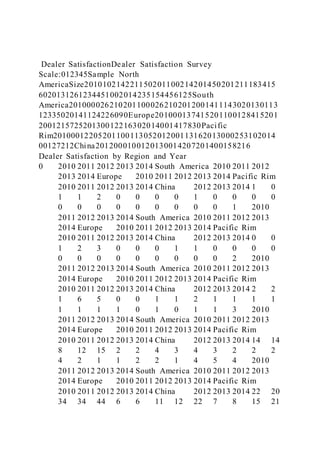
This chart is showing Dealer Satisfaction between North
America, South America, Europe, Pacific Rim and China. The
data that was selected was rated on a a survery scale from 0-5
and between the the years of 2010-2014, except for China who
started later in 2012. North America was leading in sample size
and "in 5s" dealer satisfacion for "excelltence". Although North
America recieved the highest total numbers in dealer
satisfactions for excellent rankings, in 2014, South America
recieved 60 surverys and North America recieved 56 within the
level 5 category.
End-User SatisfactionEnd-User SatisfactionSample North
America012345Size201013615373810020111241835401002012
12517344110020130241533461002014023153149100South
America2010125183638100201113617363710020120261937361
0020130252037361002014025193737100Europe2010124213636
10020111252134371002012114263731100201311317413710020
14012194533100Pacific
Rim2010235154134100201112715413410020121251640361002
0130241740371002014013194235100China20120336281050201
3122430115020140113311450
End-User Satisfaction by Region and Year
0 2010 2011 2012 2013 2014 South America 2010 2011 2012
2013 2014 Europe 2010 2011 2012 2013 2014 Pacific Rim
2010 2011 2012 2013 2014 China 2012 2013 2014 1 1
1 0 0 1 1 0 0 0 1 1 1 1
3. 0 2 1 1 0 0 0 1 0 1 2010
2011 2012 2013 2014 South America 2010 2011 2012 2013
2014 Europe 2010 2011 2012 2013 2014 Pacific Rim
2010 2011 2012 2013 2014 China 2012 2013 2014 3 2
2 2 2 2 3 2 2 2 2 2 1 1
1 3 2 2 2 1 3 2 1 2 2010
2011 2012 2013 2014 South America 2010 2011 2012 2013
2014 Europe 2010 2011 2012 2013 2014 Pacific Rim
2010 2011 2012 2013 2014 China 2012 2013 2014 6 4
5 4 3 5 6 6 5 5 4 5 4 3
2 5 7 5 4 3 3 2 1 3 2010
2011 2012 2013 2014 South America 2010 2011 2012 2013
2014 Europe 2010 2011 2012 2013 2014 Pacific Rim
2010 2011 2012 2013 2014 China 2012 2013 2014 15 18
17 15 15 18 17 19 20 19 21 21 26 17
19 15 15 16 17 19 6 4 3 4 2010
2011 2012 2013 2014 South America 2010 2011 2012 2013
2014 Europe 2010 2011 2012 2013 2014 Pacific Rim
2010 2011 2012 2013 2014 China 2012 2013 2014 37 35
34 33 31 36 36 37 37 37 36 34 37 41
45 41 41 40 40 42 28 30 31 5 2010
2011 2012 2013 2014 South America 2010 2011 2012 2013
2014 Europe 2010 2011 2012 2013 2014 Pacific Rim
2010 2011 2012 2013 2014 China 2012 2013 2014 38 40
41 46 49 38 37 36 36 37 36 37 31 37
33 34 34 36 37 35 10 11 14
This chart is showing End-User Satisfaction between North
America, South America, Europe, Pacific Rim and China. The
data that was selected was rated on a a survery scale from 0-5
and between the the years of 2010-2014, except for China who
started later in 2012. North America, South America, Europe,
and the Pacific Rim all have the same sample size of 100 for
4. each year between 2010 through 2014. China has a smaller
sample size of 50 between the years of 2012 through 2014. You
can see that the ratings of 5's, 4's, and 3's are the highest
ratings. North America's rating of 4 decreases every year
starting with 2010 while the 5 ratings increase through the
years. The Pacfic Rim's 4 ratings are highest rated and is
basically constant throughout the years while the 5 ratings are
lower then 4 ratings the 5's are constant throughout the years.
Complaints ComplaintsMonthWorldNASAEurPacChinaJan-
1016910212523Feb-1018711513554Mar-1021012815616Apr-
1022613616677May-1023213717735Jun-1026115119829Jul-
1024514018807Aug-1022312816763Sep-1019510315734Oct-
101749614622Nov-101548411590Dec-10163999541Jan-
1119512310593Feb-1122114113625Mar-1124015216666Apr-
11264163207011May-1128317822758Jun-11296170288612Jul-
11269153258110Aug-1125614623798Sep-1123113120737Oct-
1121412516685Nov-1120111813664Dec-111719611613Jan-
12200112156643Feb-12216117187164Mar-
12234126207693Apr-122531382379112May-
122821522685145Jun-123051633091156Jul-
122961562889185Aug-122791482686154Sep-
122661432482134Oct-122431312176123Nov-
122321281873103Dec-12203107157074Jan-
13216110197485Feb-132391232379104Mar-
132661382683136Apr-132841503088115May-
133151693391157Jun-133401813795198Jul-
133191693492177Aug-133041603290157Sep-
132771412987146Oct-132501232683126Nov-
132281122477105Dec-13213105237474Jan-
14240121268085Feb-142511262882105Mar-
142811483185125Apr-142981553589136May-
143221683995128Jun-1435018343981511Jul-
1433017041951410Aug-143111583893139Sep-
142891493389117Oct-14265136308586Nov-
14239121268075Dec-14219108237675
7. 41883 41913 41944 41974 3 4 6 7
5 9 7 3 4 2 0 1 3 5 6 11
8 12 10 8 7 5 4 3 4 6 9 11
14 15 18 15 13 12 10 7 8 10 13 11
15 19 17 15 14 12 10 7 8 10 12 13
12 15 14 13 11 8 7 7 China 40179
40210 40238 40269 40299 40330 40360
40391 40422 40452 40483 40513 40544
40575 40603 40634 40664 40695 40725
40756 40787 40817 40848 40878 40909
40940 40969 41000 41030 41061 41091
41122 41153 41183 41214 41244 41275
41306 41334 41365 41395 41426 41456
41487 41518 41548 41579 41609 41640
41671 41699 41730 41760 41791 41821
41852 41883 41913 41944 41974 3 4
3 2 5 6 5 4 4 3 3 4 5 4
6 5 7 8 7 7 6 6 5 4 5 5
5 6 8 11 10 9 7 6 5 5
This chart is showing PLE's Complaints from registered
customers each month within PLE's 5 regions. From this data
we can conclude that there is more use of the equipment in the
summer months because of the higher number of complaints
recieved. China has the fewest number of compaints, this is due
to the less customer usage. Based off the data, the Pacific Rim
and South America do not have as many complaints as North
America does due to less people using or purchasing PLE's
equipment. .
Mower Unit SalesMower Unit
SalesMonthNASAEuropePacificChinaWorldJan-
10600020072010007020Feb-10795022099012009280Mar-
15. 40940 40969 41000 41030 41061 41091
41122 41153 41183 41214 41244 41275
41306 41334 41365 41395 41426 41456
41487 41518 41548 41579 41609 41640
41671 41699 41730 41760 41791 41821
41852 41883 41913 41944 41974 1592
1711 1810 1867 1779 1740 1826 1695 1681 1663 1825 1720
1761 2035 2142 2340 2280 2271 2154 2146 2085 1970 1936
1850 2000 2324 2510 2672 2780 2813 2716 2581 2476 2317
2324 2080 2202 2540 2867 3348 3550 3432 3400 3261 3209
3132 3027 2777 2821 3209 3553 3820 4133 4476 4436 4256
4067 3890 3816 3717
The chart identifies the unit sales for PLE's tractor equipment.
We can see that throughout the years with the World orange line
shown in the graph increases total sales between the years of
2010 to 2014. The line is basically increase in a positive
direction on this graph. And the increase in tractor sales
increase in each region throughout the years as well. Overall
there is a positive correlations between time and tractor unit
sales over all of the country regions.
Q2Sum of PercentYear20102011201220132014Anova: Single
FactorMonthJan98.43%98.44%98.67%98.92%99.21%SUMMAR
YFeb98.09%98.63%98.79%98.82%99.14%GroupsCountSumAve
rageVarianceMar97.58%98.38%98.67%98.91%99.28%20101211
.819193754498.49%0.000012772Apr98.60%98.73%98.80%98.9
7%99.22%20111211.833727270198.61%0.0000022009May98.7
3%98.73%98.84%99.11%99.22%20121211.853179718798.78%0
.000000506Jun98.64%98.78%98.81%98.91%99.08%20131211.8
72309097698.94%0.0000034754Jul98.58%98.71%98.89%98.99
%99.23%20141211.888252856399.07%0.0000137813Aug98.67
%98.67%98.77%99.12%99.23%Sep98.94%98.58%98.77%98.93
19. 0.98890532544378695 0.98765432098765427
0.98772563176895312 0.98672566371681414
0.98825256975036713 0.98813936249073386
0.98917748917748916 0.98821796759941094
0.98905908096280093 0.98972099853157125
0.99111111111111116 0.98913830557566984
0.98994252873563215 0.99124726477024072
0.98930099857346643 0.98988439306358378
0.98427448177269483 0.99123447772096418
0.99214846538187007 0.99135446685878958
0.99283154121863804 0.99220963172804533
0.99215965787598004 0.99081272084805649
0.99228611500701258 0.99231306778476591
0.98685121107266438 0.99228070175438599
0.99292285916489742 0.98008241758241754
We decided to use a clustered column chart to represent the On-
Time deliveries for PLE's unit deliveries. The darker
backgorund makes it easier to see the difference in the
deliveries and the ones that were delivered on time to the
customer. For example, for the month of January of 2010, PLE's
had a total of 1086 deliveries but out of that number, 98.4%
when delivered on-time. This chart makes is easy to compare
those deliveries.
Response TimeResponse times to customer service callsQ1
2013Q2 2013Q3 2013Q4 2013Q1 2014Q2 2014Q3 2014Q4
20144.364.333.714.442.753.451.672.555.424.732.524.073.241.9
52.582.305.501.632.695.114.352.773.471.042.794.213.473.495.
581.833.121.595.556.895.124.692.893.721.003.113.650.921.006
.365.094.595.404.058.025.273.448.262.331.173.903.384.000.90
6.041.911.691.464.491.263.343.852.538.933.881.902.060.904.9
26. From the data in this line graph, on response time between
quarters, we are able to determine that there is no correlation
between response times and quarters from how the lines on the
graph are random.
Part 2 - Shipping CostUnit Shipping Cost PlantExisting
/ProposedCustomerMowersTractorsPlantExisting
/ProposedKansas CityExistingToronto$1.36$1.79Kansas
CityExistingSantiagoExistingToronto$1.49$2.13SantiagoExistin
gKansas
CityExistingShanghai$1.58$2.13AucklandProposedSantiagoExis
tingShanghai$1.47$2.03BirminghamProposedKansas
CityExistingMexico
City$1.32$1.76FrankfurtProposedSantiagoExistingMexico
City$1.22$1.58MumbaiProposedKansas
CityExistingMelbourne$1.72$2.34SingaporeProposedSantiagoE
xistingMelbourne$1.49$1.80Kansas
CityExistingLondon$1.49$1.86SantiagoExistingLondon$1.58$2.
14Kansas
CityExistingCaracas$1.54$1.90SantiagoExistingCaracas$1.00$1
.26Kansas
CityExistingAtlanta$1.31$1.82SantiagoExistingAtlanta$1.31$1.
76SingaporeProposedToronto$1.71$2.03BirminghamProposedT
oronto$1.34$1.78MowersTactorsFrankfurtProposedToronto$1.5
2$1.87QuartilesExistingProposedExistingProposedMumbaiProp
osedToronto$1.67$2.14125%$ 1.31$ 1.77$ 1.40$
1.78AucklandProposedToronto$1.86$2.19250%$ 1.48$ 1.84$
1.52$ 2.01SingaporeProposedShanghai$1.44$1.78375%$
1.53$ 2.11$ 1.66$
2.17BirminghamProposedShanghai$1.60$2.154100%$ 1.72$
2.34$ 1.98$
2.68FrankfurtProposedShanghai$1.65$ 2.32MumbaiProposedSha
nghai$1.21$1.47AucklandProposedShanghai$1.18$1.63Singapor
eProposedMexico City$1.72$2.09BirminghamProposedMexico
City$1.29$1.79FrankfurtProposedMexico
28. of Ease of UseAverage of
QualityChina32.64.13.8Eur3.93.86666666674.33333333334.1N
A3.714.314.274.6Pac4.14.33.94.4SA3.54.243.924.28Grand
Total3.674.144.1654.395
Average of Price China Eur NA Pac SA 3 3.9
3.71 4.0999999999999996 3.5 Average of Service
China Eur NA Pac SA 2.6 3.8666666666666667
4.3099999999999996 4.3 4.24 Average of Ease of
Use China Eur NA Pac SA 4.0999999999999996
4.333333333333333 4.2699999999999996 3.9 3.92
Average of Quality China Eur NA Pac SA 3.8
4.0999999999999996 4.5999999999999996
4.4000000000000004 4.28
Q1Anova: Single
FactorSUMMARYGroupsCountSumAverageVarianceQuality200
8794.3950.5818844221Ease of
Use2008334.1650.6108291457Price2007343.671.1367839196A
NOVASource of VariationSSdfMSFP-valueF critBetween
Groups54.9033333333227.451666666735.353118191403.01081
52042Within
Groups463.575970.7764991625Total518.4733333333599
Part 3 - 2014 Customer Survey2014 Customer SurveyQuartiles
RegionQualityEase of UsePriceServiceNorth AmericaSouth
AmericaEuropePacific RimChinaNA4134QualityEase of
UsePriceServiceQualityEase of UsePriceServiceQualityEase of
UsePriceServiceQualityEase of UsePriceServiceQualityEase of
UsePriceServiceNA444500%111200%111100%231100%323300
%2321NA4543125%4434125%4434125%4443.25125%3233125
%3.25432NA5444250%5444250%4444250%4444250%4444250
%4433NA5454375%554.255375%5445375%5554.75375%4.544
4375%4433NA55354100%55554100%55554100%55554100%54
454100%5544NA5442NA5545NA4445NA4545NA4514NA5544
29. Frequency DistrbutionNA5433North AmericaSouth
AmericaEuropePacific Rim ChinaNA4544ValueQualityEase of
UsePriceServiceValueQualityEase of
UsePriceServiceValueQualityEase of
UsePriceServiceValueQualityEase of
UsePriceServiceValueQualityEase of
UsePriceServiceNA54351125011121100211000010001NA55252
0210320180210122010021023NA5425336198346106363453111
132165NA54254304741444243523224121414144467545721NA
4544566432545521772151113985522452200NA4454NA4424N
A4334NA5525NA5343NA5445NA5525NA5553NA4454NA5444
NA5155NA5435NA4514NA4435NA5344NA5524NA5444NA55
44NA5545NA4335NA5443NA5434NA5515NA5454NA3434NA
5424NA5545NA5534NA5444NA5444NA5445NA5414 NA5455N
A5534NA5445NA4355NA5444Q1NA5555NA5545Anova:
Single
FactorNA4444NA5455SUMMARYNA4554GroupsCountSumAv
erageVarianceNA5554Quality2008794.3950.5818844221NA553
5Ease of
Use2008334.1650.6108291457NA5444Price2007343.671.13678
39196NA5452NA4455NA4445ANOVANA5444Source of
VariationSSdfMSFP-valueF critNA5435Between
Groups54.9033333333227.451666666735.353118191403.01081
52042NA5454Within
Groups463.575970.7764991625NA5545NA5444Total518.47333
33333599NA5452NA5345NA5455NA5415NA4535NA3525NA5
544NA4435NA3245NA1434NA4535NA5544NA4555NA5545N
A5544NA4245NA5454NA5454NA5543NA5555NA4553NA5545
NA4455NA5534NA4524NA5554NA4543NA4554SA5435SA542
4SA5455SA4245SA5445SA4525SA5444SA4535SA4443SA4424
SA5434SA3355SA5434SA5425SA4434SA4435SA1534SA5424S
A4444SA4455SA5424SA4455SA4443SA3345SA5444SA4441S
A4555SA4145SA4544SA4445SA5434SA4445SA5543SA5544S
A4424SA4445SA5445SA5444SA5414SA3445SA4354SA4423S
A5433SA4345SA5355SA5444SA5444SA3434SA4414SA4343Eu
r4553Eur4442Eur3454Eur3413Eur4455Eur5555Eur5551Eur4554
31. Pacific Rim
1 Quality Ease of Use PriceService 0 0 0 0
2 Quality Ease of Use PriceService 0 1 0
0 3 Quality Ease of Use PriceService 1 1
1 1 4 Quality Ease of Use PriceService 4
6 7 5 5 Quality Ease of Use PriceService
5 2 2 4
China
1 Quality Ease of Use PriceService 0 0 0 1
2 Quality Ease of Use PriceService 1 0 2
3 3 Quality Ease of Use PriceService 2 1
6 5 4 Quality Ease of Use PriceService 5
7 2 1 5 Quality Ease of Use PriceService
2 2 0 0
In this chart with the frequency distribution for North America,
you can see that the quality, ease of use, and service production
areas don't need to really change anything. Those areas can do
the same thing they are doing. The price section in this chart
needs improvment in their pricing, by the wide variation in the
distribution, you can reduce costs or use different materials.
In this chart with the frequency distribution for South America,
you can see that quality and service areas don't need to change
anything they can keep on doing what they are doing. The ease
of use can improve in turing all of those 4's into 5's for better
ratings. Price again can change by reducing costs or changing
32. materials to reduce the pricing.
In this chart with the frequency distribution shown in a
historgram for Europe region, you can see all areas; quality,
ease of use, price, and service all need improvments to get
higher ratings from consumers. Price can reduce costs. Service
can train their service workers to help customers better. Ease of
use can improve the design of the product. Quality can improve
on the procurment side to making better products.
In this chart with the frequency distribution shown in a
histogram for Pacific Rim region, you can see most of the areas
most rated number is 4's. So, service, price, and ease of use can
improve a little bit to make some of those 4's into 5's. Quality
can improve the overall quality in products from the procurment
side.
In this chart showning the China regions distribution between
areas and ratings. All areas need improvment to make the
customers want to get these products again. Quality needs to
improve the quality of the product by changing the procument
side of things. Ease of use comes from that if the quality is
good and making it easy to use will follow a little. We need to
train or hire more people to help with the companies customer
service so our customers have a good experience with our
company. Overall everything is connected so if you focus on
some areas the others will some what follow.
Unit Production CostsUnit Production
CostsMonthTractorMowerJan-10$1,750$1$50$1Feb-
10$1,755$1$50$1Mar-10$1,763$1$51$1Apr-
10$1,770$1$51$1May-10$1,778$1$51$1Jun-
10$1,785$1$51$1Jul-10$1,792$1$51$1Aug-
10$1,795$1$51$1Sep-10$1,801$1$52$1Oct-
10$1,804$1$52$1Nov-10$1,810$1$52$1Dec-
10$1,813$1$52$1Jan-11$1,835$1$55$1Feb-
11$1,841$1$55$1Mar-11$1,848$1$55$1Apr-
11$1,854$1$55$1May-11$1,860$1$56$1Jun-
11$1,866$1$56$1Jul-11$1,872$1$56$1Aug-
11$1,878$1$56$1Sep-11$1,885$1$56$1Oct-
58. 21469.377637268572 21127.340647579105
20527.194347858862 19793.626314204532
18332.973158006946 18314.484223735177
20481.032187050154 22493.666036040744
23612.032608397036 25443.736066418991
27378.895949558133 26768.988797130431
25432.686015877025 24000.046319474648
23146.724604316583 22670.622639347333
21993.298087858158
Q3Anova: Single
FactorSUMMARYGroupsCountSumAverageVariance201012991
6826.3333333333135.333333333320111210049837.4166666667
121.53787878792012129431785.91666666672749.71969696972
013128029669.0833333333959.35606060612014125955496.252
940.0227272727ANOVASource of VariationSSdfMSFP-valueF
critBetween
Groups984600.3333333334246150.083333333178.2154383340.
00002.5396886349Within
Groups75965.6666666667551381.1939393939Total106056659
Defects After DeliveryDefects After DeliveryDefects per
million items received from
suppliersMonth20102011201220132014January81282882468257
1February810832836695575March813847818692547April82383
9825686542May832832804673532June848840812681496July83
7849806696472August831857798688460September8278398046
71441October838842713645445November826828705617438Dec
ember819816686603436Total
991610049943180295955Q3Anova: Single
FactorSUMMARYGroupsCountSumAverageVariance201012991
6826.3333333333135.333333333320111210049837.4166666667
121.53787878792012129431785.91666666672749.71969696972
013128029669.0833333333959.35606060612014125955496.252
940.0227272727ANOVASource of VariationSSdfMSFP-valueF
59. critBetween
Groups984600.3333333334246150.083333333178.2154383340.
00002.5396886349Within
Groups75965.6666666667551381.1939393939Total106056659w
e conduct two regression analyses (i) what may have happened
had the supplier initiative not been impelemented (ii) how the
number of defects might further be reduced in the future.i) what
might have happened had the supplier initiative not been
implemented here the analysis is based on months from January
2010 to when the supplier initiative was done in august 2011.
Let t be the number of months from December 2009; that is
January 2010 be t=1, February 2010 be t=2 and so onDefects
per million items received from suppliers is the dependent
variabe while time is the independent variableDefectstime
t8121810281338234832584868377831882798381082611819128
281383214847158391683217840188491985720The following is
the regression equationSUMMARY OUTPUTRegression
StatisticsMultiple R0.6994187048R
Square0.4891865246Adjusted R Square0.4608079981Standard
Error9.4427395385Observations20ANOVAdfSSMSFSignificanc
e
FRegression11537.02406015041537.024060150417.2379114202
0.0005989968Residual181604.975939849689.1653299916Total
193142CoefficientsStandard Errort StatP-valueLower 95%Upper
95%Lower 95.0%Upper
95.0%Intercept816.03684210534.3864495472186.03584364355.
14111788361825E-
31806.8212535732825.2524306373806.8212535732825.252430
6373X Variable
11.52030075190.36617373334.15185638240.00059899680.7509
9828492.28960321880.75099828492.2896032188Regression
Equationy=1.520301x + 816.0368defects= 1.520301* t +
816.0368This means had the supplier initiative not taken place,
the number of defects would have increased with timewhere t is
the number of months from the baseline.had the supplier
initiative of August 2011 not taken place, this regression
60. equation would have predicted what would have happened in
subsequent months after august 2011ii)how the number of
defects might further be reduced in the futurehere we analyze
regression resuts from september 2011 when the supplier
initiative was undertakenthe new baseline is august 2011, so for
september 2011, t=1, october 2011 t=2, and so on. DefectsTime
t8391842282838164824583668187825880498121080611798128
04137131470515686166821769518692196862067321681226962
36882467125645266172760328571295753054731542325323349
634472354603644137445384383943640The regression results
are:SUMMARY OUTPUTRegression StatisticsMultiple
R0.9750468977R Square0.9507164528Adjusted R
Square0.9494195173Standard
Error30.1520143865Observations40ANOVAdfSSMSFSignifican
ce
FRegression1666446.529080675666446.529080675733.0483948
9421.90959818846179E-
26Residual3834547.4709193246909.1439715612Total39700994
CoefficientsStandard Errort StatP-valueLower 95%Upper
95%Lower 95.0%Upper
95.0%Intercept897.73076923089.71653769392.39204309162.48
445466444305E-
46878.0606670317917.4008714299878.0606670317917.400871
4299X Variable 1-11.1819887430.4130025443-
27.07486647971.9095981884618E-26-12.0180686833-
10.3459088026-12.0180686833-10.3459088026The value of R-
squared means the model is a good fit for the data.The p-values
indicate statistical significanceRegression Equationy=-11.182X
+897.7308defects=897.7308-11.182*there t is the number of
months from august 2011
Defects After Delivery by Year
2010 2011 2012 2013 2014 9916 10049 9431 8029 5955 2010
2011 2012 2013 2014 812 828 824 682 571 2010 2011
2012 2013 2014 810 832 836 695 575 2010 2011 2012
2013 2014 813 847 818 692 547 2010 2011 2012 2013
2014 823 839 825 686 542 2010 2011 2012 2013 2014
61. 832 832 804 673 532 2010 2011 2012 2013 2014 848
840 812 681 496 2010 2011 2012 2013 2014 837 849
806 696 472 2010 2011 2012 2013 2014 831 857 798
688 460 2010 2011 2012 2013 2014 827 839 804 671
441 2010 2011 2012 2013 2014 838 842 713 645 445
2010 2011 2012 2013 2014 826 828 705 617 438 2010
2011 2012 2013 2014 819 816 686 603 436
We can conclude that Defects had a slight increase from 2010 to
2011 which can be attributed to an increase in unit sales. But
over the years from the years of 2010 to 2014 the amount of
defects decreased overall . This shows that the company is
evolving and improving their manufacturing process.
Time to Pay SuppliersTime to Pay SuppliersMonthWorking
DaysJan-108.32Feb-108.28Mar-108.29Apr-108.32May-
108.36Jun-108.35Jul-108.34Aug-108.32Sep-108.36Oct-
108.33Nov-108.32Dec-108.29Jan-117.89Feb-117.65Mar-
117.58Apr-117.53May-117.48Jun-117.45Jul-117.36Aug-
117.35Sep-117.32Oct-117.3Nov-117.27Dec-117.25Jan-
127.22Feb-127.21Mar-127.22Apr-127.29May-127.25Jun-
127.23Jul-127.28Aug-127.25Sep-127.24Oct-127.26Nov-
127.21Dec-127.23Jan-137.24Feb-137.19Mar-137.21Apr-
137.23May-137.22Jun-137.19Jul-137.17Aug-137.15Sep-
137.16Oct-137.16Nov-137.15Dec-137.14Jan-147.12Feb-
147.11Mar-147.11Apr-147.11May-147.11Jun-147.12Jul-
147.08Aug-147.09Sep-147.09Oct-147.04Nov-147.06Dec-147.08
Employee SatisfactionEmployee Satisfaction ResultsAverages
using a 5 point scaleDesign &Sales & QuarterProductionSample
sizeManagerSample sizeAdministrationSample sizeTotalSample
size1st Q-112.861003.81103.51303.071402nd Q-
112.911003.76103.38303.071403rd Q-
112.841003.86103.45303.041404th Q-
112.831003.48103.61303.041401st Q-
62. 122.911003.75203.37303.111502nd Q-
122.941003.92203.53303.191503rd Q-
122.861003.89203.47303.121504th Q-
122.831003.58203.66303.101501st Q-
132.951003.82203.71403.251602nd Q-
133.011004.01203.53403.271603rd Q-
133.031003.92203.62403.291604th Q-
132.961003.84203.48403.201601st Q-
143.051003.92203.52403.281602nd Q-
143.121004.00203.37403.291603rd Q-
143.061003.93203.46403.271604th Q-
143.021003.70203.59403.25160
EnginesEngine Production TimeSampleProduction Time
(min)165.1time is the dependent variable and sample is the
independent variable262.3360.4SUMMARY
OUTPUT458.7558.1Regression Statistics656.9Multiple
R0.9213573188757.0R Square0.8488993088856.5Adjusted R
Square0.8457513778955.1Standard
Error1.81826878671054.3Observations501153.71253.2ANOVA
1352.8dfSSMSFSignificance
F1452.5Regression1891.5529337335891.5529337335269.66896
386722.48594348198823E-
211552.1Residual48158.69286626653.30610138061651.8Total4
91050.24581751.51851.3CoefficientsStandard Errort StatP-
valueLower 95%Upper 95%Lower 95.0%Upper
95.0%1950.9Intercept58.18367346940.5220964329111.4423884
2141.29129366690705E-
5957.133928234659.233418704257.133928234659.2334187042
2050.5X Variable 1-0.29261464590.0178188871-
16.4216005272.48594348198821E-21-0.3284419196-
0.2567873721-0.3284419196-0.25678737212150.22250.0The
value of R-squared means the model is a good fit for the
data.2349.7The p-values indicate statistical
significance2449.52549.3The regression equation is :
y=58.18367-0.29261x2649.4Production Time=58.18367-
0.29261*x2749.1This means that as the number of units
63. produced increase, the production time reduces and therefore
creating a more cost-effective means of
production2849.02948.83048.53148.33248.23348.13447.93547.
73647.63747.43847.13946.94046.84146.74246.64346.54446.545
46.24646.34746.04845.84945.75045.6
Q4Anova: Single
FactorSUMMARYGroupsCountSumAverageVarianceCurrent308
688289.62061.1448275862Process
A308565285.54217.6379310345Process
B308953298.4333333333435.3574712 644ANOVASource of
VariationSSdfMSFP-valueF critBetween
Groups2621.088888888921310.54444444440.58557509950.558
96481053.1012957567Within
Groups194710.066666667872238.046743295Total197331.15555
555689
Transmission CostsUnit Tractor Transmission
CostsQ4CurrentProcess AProcess
B$242.00$242.00$292.00Anova: Single
Factor$176.00$275.00$321.00$286.00$199.00$314.00SUMMA
RY$269.00$219.00$242.00GroupsCountSumAverageVariance$3
27.00$273.00$278.00Current308688289.62061.1448275862$264
.00$265.00$300.00Process
A308565285.54217.6379310345$296.00$435.00$301.00Process
B308953298.4333333333435.3574712644$333.00$285.00$286.0
0$242.00$384.00$315.00$288.00$387.00$300.00ANOVA$314.0
0$299.00$304.00Source of VariationSSdfMSFP-valueF
crit$302.00$145.00$300.00Between
Groups2621.088888888921310.54444444440.58557509950.558
96481053.1012957567$335.00$266.00$351.00Within
Groups194710.066666667872238.046743295$242.00$216.00$2
77.00$281.00$331.00$284.00Total197331.15555555689$289.00
$247.00$276.00$259.00$280.00$312.00$322.00$267.00$273.00
$209.00$210.00$281.00$282.00$391.00$303.00$304.00$297.00
$306.00$391.00$346.00$312.00$236.00$230.00$287.00$383.00
$332.00$306.00$299.00$301.00$312.00$300.00$277.00$295.00
$278.00$336.00$288.00$303.00$217.00$313.00$315.00$274.00
64. $286.00$321.00$339.00$338.00
Blade WeightBlade Weight SampleWeight14.88Question 4(
Average blade weight)24.92we use the average function in
Excel35.02average blade weight4.990844.9755.00for
variability, we use the sample standard
deviation64.99s.d.0.1092875674.8685.0795.04QUESTION 5
(probability blade weights will exceed 5.20)104.87we calculate
the z-score associated with
5.20114.77z1.9142160368125.14probability
(Z.Z>1.914216)0.027796135.04145.00154.88QUESTION 6
(probability blade weights will be less than
4.80)164.91175.09we calculate the z-score associated with
4.80184.97z-1.7458528672194.98probability (Z<-
1.74585)0.0404182609205.07215.03QUESTION 7 (actual
pecentage less than 4.80 or greater than 5.20)225.12235.08less
than 4.808244.86more than
5.207255.11total15264.92275.18actaul percentage <4.80 or >
5.204.2857%284.93295.12305.08QUESTION 8 (is the process
stable over time)314.75we can make a scatter plot to investigate
the stability of the
process324.99335.00344.91355.18364.95374.63384.89395.1140
5.05415.03425.02434.96445.04454.93465.06475.07485.00495.0
3505.00514.95from the scatter plot, we can observe that the
process is quite stable because most values are close to each
other524.99535.02544.90Question 9 (are there any
outliers)555.105.87565.01yes, there are possible outliers. For
example,the 171st blade with a weight of 5.87 is an outlier
because it is far from the other
values.574.84585.01594.88QUESTION 10 (Is the distribution
normal)604.97beloe mean180614.97above
mean170625.06635.06since the number of values below the
mean is close to the number of values above the mean, the
distribution is pretty
normal645.04654.87665.00675.03685.02695.02705.06715.2172
5.09734.97745.01754.90764.89774.93785.16795.02805.01815.1
0825.03835.07844.92855.08864.96874.74884.91895.12905.0091