2. layers with subnanometer resolution. However, due to the loss of
phase information in the process, analysis of the XRR data will be
model dependent.
In the present article, our objective is to obtain an electron
density profile (EDP), thickness, and roughness of the nanostructured
ultra-thin films prepared by spray pyrolysis method. The effect of
precursor volume (PV) and PC on the thin film structures will be inves-
tigated by considering their XRR curves. The sheet resistance of the
samples was measured by the four-probe method, and the results
were interpreted concerning the corresponding EDPs deduced from
XRR data.
2 | EXPERIMENTAL SECTION
Two sets of samples were prepared and considered. The first set
includes four samples (named A–D) with PV of varying from 20 to
50 mL with an increment of 10 mL. In this set, PC is 0.01 M. The
second set includes samples (named–H) with the same PV condition
as the first set but possessing a higher PC = 0.05 M. To produce a pre-
cursor solution, SnCl2 2H2O was dissolved in 3 mL of concentrated
hydrochloric (HCl) acid. The resultant transparent solution was then
diluted with methanol to form 0.01 M (Set 1) and 0.05 M (Set 2)
starting precursor solutions. In this study, the precursor solutions used
to spray perpendicularly onto the substrates of microscopic glass
slides (75 × 25 × 1.4 mm3
). The substrates were cleaned using
deionized distilled water and various organic solvents. The tempera-
ture of the substrates was kept at 450
C. The compressed ambient air
supplied by an air compressor was utilized to atomize the solution.
The carrier gas (air) flow rate was maintained at 3 mL/min at a
pressure of 1 atm. The distance between the spray nozzle and the
substrate is fixed at 40 cm.
In this work, a model consisting of layers of constant electron
density was utilized for which the Vidal and Vincent matrix model12
can be employed. A model to describe the EDP of the deposited
layers using complementary error function at the interfaces of
substrate-film and film-vacuum was presented:
ρ z
ð Þ =
1
2
X
i
δρ z
ð Þerfc
z−zi
ffiffiffi
2
p
σi
, ð1Þ
where δρ(z) is the electron density difference between two adjacent
layers and σi is the root mean square roughness of the interface i.
A high-resolution diffractometer, with a copper X-ray tube
(λ = 1.54 Å) at the Physics Department of McGill University, Montreal,
Quebec, Canada, is used to take the XRR data. In this setup, two
germanium crystals acting as analyzer and monochromator with a
3 × 10⁻⁵
rad width for their (111) reflection are used. At each detec-
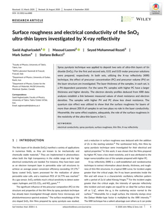
tor position (each 2θ), a θ-rocking scan around ω = 0 (θ = 2θ
2 Þ was done
and then the diffuse part of the scattering was separated (Figure 1).
The remaining specular part can be approximated by a Gaussian curve,
where an average diffuse background line was approximated (insets in
Figure 1) and subtracted from each point in the specular-θ-rocking
curve. Finally, the surface area under the obtained curve is calculated
to give the specular intensity. The crystallographic nature of SnO2 thin
films was studied by the X-ray diffraction (XRD) technique using
Cu-Kα target (λ = 1.54 Å) utilizing X-Pert Pro X-ray diffractometer.
3 | RESULTS AND DISCUSSION
3.1 | XRD analysis
Figure 2 demonstrates the XRD pattern of the SnO2 thin films for
samples in Set 2 with various PVs along with the standard profile of
SnO2 generated from a space group analysis.13
The presence of the
main diffraction peaks in the sample with 50 mL of PV is assigned to
the miller indices of (110) and (101). Two small peaks that happened
at 2θ = 26.60
, for PV = 30 and 40 mL, are indications of a small
FIGURE 1 The θ-rocking curves at 2θ = 1
for 20-, 30-, 40-, and
50-mL samples (first set). The insets illustrate a Gaussian fit (black
line) for the specular parts, and the arrows point the background line
2 ASGHARIZADEH ET AL.
3. percentage of crystallites of (110) Bragg reflection. The XRD pattern
of the samples in Set 1 resembles the ones in Set 2 with no peaks and
are not shown. Using the Scherrer equation, D = 0:9λ
βcosθ , the crystallite
size of the deposited layer was calculated. In the formula, λ is the
X-ray wavelength, β is the full width at half maximum (FWHM) of the
(110) reflection peak in radian, and θ is the Bragg's angle. The
calculated crystallite size was 44.6 nm. It will be discussed in the next
paragraphs that increasing the PV will lead to thicker samples in the
deposition process. As the film thickness increases, the crystallinity of
the film is also improved. This is due to the fact that in the thicker
samples, compared with the thinner ones, small size crystallites have
more chance to agglomerate and coalesce together to enhance the
crystallite structure.
3.2 | XRR analysis
Figure 3A depicts the measured experimental XRR curves (hallow
dots) for samples within Set 1 and the best theoretical fits (solid lines).
In this figure, the intensity of the reflected beam is shown versus
momentum transferred to the film in the direction perpendicular to
the film surface qz = 4π
λ sinθ: The corresponding EDPs are shown in
Figure 3B. In the model presented, each interface is described via a
complementary error function, so a Gaussian profile for dρ/dz at the
interfaces is expected. The XRR curve of the bare substrates was
measured, and root mean square roughness of 5–9 Å was obtained.
From the same curve, the electron density of the glass substrates is
calculated to be 0.71 e/Å3
. The parameters obtained by fitting XRR
curves for Set 1 of the samples are summarized in Table 1. The EDPs
are featured with a plateau region corresponding to the layer density
and two sigmoid-like shapes at the interfaces. For sample A, the root
mean square surface roughness is comparable with the surface rough-
ness of the substrate, indicating that the overlayer partially replicates
the structure of the underlying interface. In samples B and C, it is dis-
cernible that the thickness is doubled compared with sample A, while
the electron density increase is not palpable. As such, one could
accentuate that the effect of the PV change on layer thickness is by
far pronounced than that on the layer density. The XRR curve of
FIGURE 2 XRD pattern of the second set of the samples
FIGURE 3 A, X-ray specular
reflectivity of the first sample set (hollow
dots) and their theoretical fits (solid lines).
The PC = 0.01 M, and the PV = 20,
30, 40, and 50 mL for samples A–D,
respectively. B, Electron density profile of
the samples in Set 1
ASGHARIZADEH ET AL. 3
4. sample D, in Figure 3A, reveals more fringes and higher amplitude of
the oscillations. The larger oscillation amplitude is associated with a
higher electron density contrast between the layer and substrate.
Besides, the presence of more interference modes of electromagnetic
waves in the layer could be attributed to the relatively big thickness
of the layer. At the same time, a big root mean square of surface
roughness deduced from the XRR data fitting (see Table 1) implies a
noticeable specular intensity diminishing in the XRR curve for this
sample. It also appears that the oscillation amplitudes are smeared out
for large qzs, due to the large surface roughness. In this set of samples,
increasing the PV to 50 mL doubles the thickness compared with the
samples B and C (Table 1 and Figure 3B).
Figure 4 illustrates the evolution of the layer thickness and den-
sity as a function of PV for the four samples within the same frame.
While the thickness reaches to as fourfold as its initial value, the layer
density only shows an almost 12% growth.
Figure 5A depicts XRR curves and their theoretical fits of samples
E and F. As seen, the reflectivity curve of sample F goes down faster,
at large values of scattering vectors, compared with sample E. This
indicates that the surface roughness of sample F is higher than that of
sample E.
The calculated surface roughness for samples E and F are 25 and
32 Å, respectively. Calculating the electron densities points out denser
structures compared with the samples in Set 1. These values are
1.5 e/Å3
for sample E and 1.55 e/Å3
for sample F (see Figure 5B).
Because samples in Set 2 have been prepared with a higher PC, it is
reasonable to imagine that each droplet on the substrate, in the
process of deposition, contains a higher number of solute particles.
This noticeably facilitates the process of joining the individual islands
on the substrate and results in a remarkably compact structure. The
thickness of the deposited thin layers (E: 173 Å, F: 318 Å) remarkably
shows a significant rise compared with the corresponding samples in
Set 1 with the same PV.
We tried to take XRR data for samples G and H. However, the
X-ray fringes were not displayed. This is due to a big root mean square
roughness of their surfaces. The XRR from a layer is proportional to
the Fourier transform of the gradient of EDP normal to the surface.11
An error function can describe a rough interface, then dρ/dz will be
presented by a Gaussian one. The Fourier transform of a Gaussian
function is a Gaussian, too. Consequently, the specular X-ray scatter-
ing falls as qz
−4
e− qzσ
ð Þ2
, legitimating a fast drop in specular XRR for
surfaces of big roughness. Based on this, EDP information cannot be
available for the samples G and H. Despite this conclusion, it is under-
standable that these samples will be quite thicker than E and F.
3.3 | Sheet resistance measurements
The attained values of sheet resistance are plotted in Figure 6. It can
be concluded that thicker samples have less sheet resistance for both
sample sets. This conclusion could be supported by the idea that
thicker samples contain more electrons per unit volume, which will
assist the conduction process. Denser structures will provide more
pathways for charge carriers to go through and then lower the sheet
resistance.
The sheet resistances shown in Figure 6 are identified by two
regions with two different slopes. In the first region, the sheet
resistance decreases from 25.9 MΩ/□□ to 5.84/□□, in the first sam-
ple set, and from 1.14 MΩ/□□ to 0.1 MΩ/□□, in the second sample
set. In the second region, the sheet resistance goes down smoothly.
The significant apportionment of the sheet resistance is due to the
formation process of the SnO2 layer on the glass substrate. There are
evidences14
corroborate that films of a few tens of angstrom thick or
thinner are arranged by small, individual islands separated from each
other by distances of the order of about 100 Å. To establish the elec-
trical conduction in the film, electrons have to be transferred between
the islands across the gaps, and this transfer will determine the con-
ductivity of the film. Based on a simulation done for the spray pyroly-
sis deposition method,15
droplets evaporate before reaching the
substrate and precipitate forms. Then the precipitate will be
TABLE 1 Parameters obtained from XRR data for samples with PC = 0.01 M
Sample PV (mL) Roughness (RMS) (Å) Electron density (e/Å3
) Thickness (Å) Resistivity (Ω-cm)
A 20 6 ± 1 1.20 ± 0.01 50 ± 2.0 12.9 ± 0.2
B 30 15 ± 1 1.25 ± 0.02 99 ± 1.0 5.8 ± 0.2
C 40 22 ± 1 1.30 ± 0.01 107 ± 1.0 4.7 ± 0.3
D 50 24 ± 1 1.35 ± 0.02 215 ± 2.0 8.6 ± 0.1
FIGURE 4 Thickness and electron density of the deposited layers
versus PV
4 ASGHARIZADEH ET AL.
5. converted to a vapor state near the substrate, and adsorbed
molecules on the surface of the substrate will be designed as islands
on the substrate surface.
Starting the deposition, the SnO2 particles were expected to
deposit islands on the glass substrate (first step). Continuing the
deposition with higher PVs, the gap between distant SnO2 islands was
reduced, and finally, the SnO2 islands coalesced. In this step, the
conductivity of the thin layers would be described by the following
equation16
:
σ / exp −2αs−
W
kT
, ð2Þ
where α is the tunneling exponent of electron wave functions in the
insulator, which would be an order of 1010
m−1
for an insulator16
; s is
the separation of islands; W is the island charging energy, which is
inversely proportional to the island size; k and T are the Boltzmann
constant and temperature, respectively. In the above equation, two
elements shape the conductivity: quantum tunneling, which plays a
role in electron transferring between islands, and activation energy to
create a charge carrier associated with placing an electronic charge on
an island. As the interisland separation is inversely proportional to the
island size, one can expect that decreasing the island separation
(increasing the island size) will elevate the tunneling probability in the
ultrathin layers. By utilizing higher PVs, the space between the islands
decreases, and a network structure is established, then the sheet
resistance declines.
The growth progress and surface roughness of the thin layers
govern their electrical properties. By completing the growth steps of a
layer, its conductivity could be described by the quantum size
effect.17
This effect is modeled by Fuchs–Sondheimer (F. S) describing
the behavior of the electrical resistivity as a function of the film
thickness and surface roughness. The limiting form of the F. S model
for very thin layers (k 1) is
ρ
ρ0
=
4
3
1−p
ð Þ
1 + p
ð Þ
1
k log 1
k
, ð3Þ
and for relatively thick films (k 1) is
ρ
ρ0
= 1 +
3
8
1−p
ð Þ
k
, ð4Þ
where ρ/ρ0 is the ratio between the film and bulk resistivity; k = d/λ,
d is the thickness of the film, and λ is the electron mean free path;
p (0 ≤ p ≤ 1) is the specular parameter, defined as the ratio of the
specularly scattered electrons to the total number of reflected ones.
The specular parameter p = 0 stands for a completely diffusive
scattering, while p = 1 describes a completely specular scattering.
For thick films, the specular scattering of the electrons will represent
structures with bulk conductivity. However, diffuse scattering of the
electrons at the interfaces, as a primary mechanism affecting the
resistivity, will reduce the conductivity. At the same time, for very
thin layers, the surface roughness plays an essential role in resistiv-
ity. As for a set of complete specular scattering of the elec-
trons (p = 1), the model predicts a perfect conductive layer with no
resistivity.
The resistivity of the layers can be calculated through the relation
ρ = Rsd, where Rs is the measured sheet resistance. The tabulated
FIGURE 5 A, X-ray specular
reflectivity of the second sample set. The
PC = 0.05 M, and the PV = 20, and 30 mL
for samples E and F, respectively.
B, Electron density profile of the samples
of Set 2 (PC = 0.05 M)
FIGURE 6 The sheet resistance of the thin layers versus PV. The
error bars are less than the legend size
ASGHARIZADEH ET AL. 5
6. resistivity of the samples in Set 1 (Table 1) experiences a decline with
increasing thickness up to about 100 Å after which the resistivity
escalates up. This behavior can be explained by the quantum size
effect through Equation 3. For the samples in set two, the resistivity
of ρ = 1.97 and ρ = 0.32 Ω-cm can be calculated for samples E and F,
respectively. The latter is very close to the bulk resistivity of SnO2
(ρbulk = 0.33 Ω-cm).18
Therefore, considering the Equation 4, one can
expect that the surface roughness of the samples G and H plays no
role in the layer resistivity, and the bulk properties dominate. Based
on this, missing information on layer thicknesses when the XRR
technique is used can be obtained by utilizing the relation between
resistivity and sheet resistance. The values of dG = 785 and
dH = 1,220 Å were estimated.
4 | CONCLUSION
Two sets of the ultra-thin layers prepared by the spray pyrolysis
method were investigated. EDP of the samples deduced from fitting
the XRR data shows that the samples with 0.05 M will produce denser
layers. Varying the PV affects, significantly, the thickness of the layers
and has a negligible effect on the layer density. Meanwhile, altering
the PC mainly changes the layer density. Equally important is that
using higher PCs will lead to layers with less sheet resistance. The
sheet resistance behavior of the thin layers was associated with the
layer growth procedure. In the first step of the growth, the high sheet
resistance of the ultra-thin layers was due to the sizeable interisland
separation. Utilizing higher PVs, the film growth enters into the
second step, where a network structure is formed on the substrate. In
this step, the role of the surface roughness and layer thickness in
conductivity was discussed via quantum size effect and concluded
that the surface roughness for layers of more than almost 200 Å,
prepared by higher PC, has no control over the conductivity. In this
case, the resistivity of the films approaches that of the bulk one. In
contrast, for very thin layers prepared by PC = 0.01 M, the presence
of the surface roughness is crucial in modeling the resistivity.
ORCID
Saeid Asgharizadeh https://orcid.org/0000-0003-0802-4288
Masoud Lazemi https://orcid.org/0000-0003-0118-7113
REFERENCES
1. Comini E, Faglia G, Sberveglieri G, Pan Z, Wang ZL. Stable and highly
sensitive gas sensors based on semiconducting oxide nanobelts. Appl
Phys Lett. 2002;81(10):1869-1871.
2. Jiang Q, Zhang X, You J. SnO2: a wonderful electron transport layer for
perovskite solar cells. Small. 2018;14(31):1801154-1-1801154-14.
https://doi.org/10.1002/smll.201801154
3. Taheri B, Calabrò E, Matteocci F, et al. Automated scalable
spray coating of SnO2 for the fabrication of low-temperature
perovskite solar cells and modules. Energ Technol. 2020;8(5):
1901284-1-1901284-9. https://doi.org/10.1002/ente.201901284
4. Nguyet QTM, van Duy N, Manh Hung C, Hoa ND, van Hieu N.
Ultrasensitive NO2 gas sensors using hybrid heterojunctions of
multi-walled carbon nanotubes and on-chip grown SnO2 nanowires.
Appl Phys Lett. 2018;112(15):153110-1-153110-5. https://doi.org/
10.1063/1.5023851
5. Murata N, Suzuki T, Kobayashi M, Togoh F, Asakura K. Characteriza-
tion of Pt-doped SnO2 catalyst for a high-performance micro gas sen-
sor. Phys Chem Chem Phys. 2013;15(41):17938-17946. https://doi.
org/10.1039/C3CP52490F
6. Liu B, Luo Y, Li K, Wang H, Gao L, Duan G. Room-temperature NO2
gas sensing with ultra-sensitivity activated by ultraviolet light based
on SnO2 monolayer array film. Adv Mater Interfaces. 2019;6(12):
1900376-1-1900376-10. https://doi.org/10.1002/admi.201900376
7. David Prabu R, Valanarasu S, Ganesh V, Shkir M, AlFaify S,
Kathalingam A. Investigation of molar concentration effect on struc-
tural, optical, electrical, and photovoltaic properties of spray-coated
Cu2O thin films. Surf Interface Anal. 2018;50(3):346-353.
8. Rozati SM, Shadmani E. Study on surface morphology of nanoscale
structure of pure and zinc-doped tin oxide uniform thin films. Surf
Interface Anal. 2010;42(6-7):1160-1162.
9. Choudhury SP, Gunjal SD, Kumari N, Diwate KD, Mohite KC,
Bhattacharjee A. Facile synthesis of SnO2 thin film by spray pyrolysis
technique, investigation of the structural, optical, electrical properties.
Mater Today Proc. 2016;3(6):1609-1619.
10. Kiessig H. Untersuchungen zur Totalreflexion von Röntgenstrahlen.
Ann Phys. 1931;402(6):715-768.
11. Sinha SK, Sirota EB, Garoff S, Stanley HB. X-ray and neutron
scattering from rough surfaces. Phys Rev B. 1988;38(4):2297-2311.
12. Vidal B, Vincent P. Metallic multilayers for x rays using classical
thin-film theory. Appl Optics. 1984;23(11):1794-1801. https://doi.
org/10.1364/AO.23.001794
13. Momma K, Izumi F. VESTA 3for three-dimensional visualization of
crystal, volumetric and morphology data. J Appl Cryst. 2011;44(6):
1272-1276.
14. Venables J. A. Introduction to surface and thin film processes, 2000.
15. Filipovic L, Selberherr S, Mutinati GC, et al. Methods of simulating
thin film deposition using spray pyrolysis techniques. Microelectron
Eng. 2014;117:57-66.
16. Adkins CJ. Conduction in granular metals-variable-range hopping in a
Coulomb gap? J Phys Condens Matter. 1989;1(7):1253-1259.
17. Tellier CR, Tosser AJ. Size Effects in Thin Films. Elsevier; 1982.
18. Jarzebski ZM. Physical properties of SnO2 materials: II. electrical
properties. J Electrochem Soc. 1976;123(9):299C-310C.
How to cite this article: Asgharizadeh S, Lazemi M, Rozati SM,
Sutton M, Bellucci S. Surface roughness and electrical
conductivity of the SnO2 ultra-thin layers investigated by
X-ray reflectivity. Surf Interface Anal. 2020;1–6. https://doi.
org/10.1002/sia.6888
6 ASGHARIZADEH ET AL.