Chem modiagram en

modiagram
v0.2g 2015/09/23
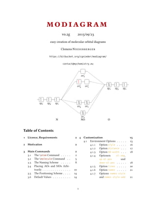
easy creation of molecular orbital diagrams
Clemens Niederberger
https://bitbucket.org/cgnieder/modiagram/
contact@mychemistry.eu
2pz2py2px
2pz2py2px
2σx
2σ∗
x
2πy
2π∗
y
2πz
2π∗
z
N NO O
Table of Contents
1 Licence, Requirements 2
2 Motivation 2
3 Main Commands 2
3.1 The atom Command . . . . . 2
3.2 The molecule Command . . 5
3.3 The Naming Scheme . . . . . 8
3.4 Placing AOs and MOs Arbi-
trarily . . . . . . . . . . . . . . 10
3.5 The Positioning Scheme . . . . 14
3.6 Default Values . . . . . . . . . 14
4 Customization 15
4.1 Environment Options . . . . . 15
4.1.1 Option style . . . . . 16
4.1.2 Option distance . . . 17
4.1.3 Option AO-width . . . 18
4.1.4 Optionen el-sep,
up-el-pos und
down-el-pos . . . . . 18
4.1.5 Option lines . . . . . 20
4.1.6 Option names . . . . . 21
4.1.7 Options names-style
and names-style-add 21
1

1 Licence, Requirements
4.1.8 Option labels . . . . 24
4.1.9 Option labels-fs . . 24
4.1.10 Option labels-style 25
4.2 atom and molecule Specific
Customizations . . . . . . . . 25
4.2.1 The label Key . . . . 25
4.2.2 The color Key . . . . 27
4.2.3 The up-el-pos and
down-el-pos keys . . 27
4.3 AO Specific Customizations . 27
4.3.1 The label Key . . . . 28
4.3.2 The color Key . . . . 28
4.3.3 The up-el-pos and
down-el-pos Keys . . 28
4.4 Energy Axis . . . . . . . . . . 28
5 Examples 30
References 33
Index 34
1 Licence, Requirements
Permission is granted to copy, distribute and/or modify this software under the terms of the LATEX
Project Public License (LPPL), version 1.3 or later (http://www.latex-project.org/lppl.txt).
The software has the status “maintained.”
modiagram uses l3kernel [L3Pa] and l3packages [L3Pb]. It also uses TikZ [Tan13] and
the package chemgreek [Nie15] bundle. Additionally the TikZ libraries calc and arrows are
loaded. Knowledge of TikZ is helpful.
2 Motivation
This package has been written as a reaction to a question on http://tex.stackexchange.com/.
To be more precise: as a reaction to the question “Molecular orbital diagrams in LaTeX.” There
it says
I’m wondering if anyone has seen a package for drawing (qualitative) molecular orbital
splitting diagrams in LATEX? Or if there exist any packages that can be easily re-purposed
to this task?
Otherwise, I think I’ll have a go at it in TikZ.
The problem was solved using TikZ, since no package existed for that purpose. For one thing
modiagram is intended to fill this gap. I also found it very tedious, to make all this copying
and pasting when I needed a second, third, ... diagram. modiagram took care of that.
3 Main Commands
All molecular orbital (MO) diagrams are created using the environment MOdiagram.
3.1 The atom Command
atom[ name ]{ left | right }{ AO-spec }
Place an AO in the diagram. name is caption of the atom, left and right determine the
placement in the diagram, AO-spec is the specification of the AO.
2

3 Main Commands
Let’s take a look at an example:
1 begin{MOdiagram}
2 atom{right}{
3 1s = { 0; pair} ,
4 2s = { 1; pair} ,
5 2p = {1.5; up, down }
6 }
7 end{MOdiagram}
As you can see, the argument AO-spec is essential to create the actual orbitals and the
electrons within. You can use these key/value pairs to specify what you need:
1s = { rel-energy ; el-spec }
Energy level and electron specifications for the 1s orbital.
2s = { rel-energy ; el-spec }
Energy level and electron specifications for the 2s orbital.
2p = { rel-energy ; x el-spec , y el-spec , z el-spec }
Energy level and electron specifications for the 2p orbitals.
el-spec can have the values pair, up and down or can be left empty. rel-energy actually is the
y coordinate and shifts the AO vertically by rel-energy cm.
The argument left / right is important, when p orbitals are used. For instance compare the
following example to the one before:
1 begin{MOdiagram}
2 atom{left}{
3 1s = { 0; pair} ,
4 2s = { 1; pair} ,
5 2p = {1.5; up, down }
6 }
7 end{MOdiagram}
When both variants are used one can also see, that the right atom is shifted to the right (hence
the naming). The right atom is shifted by 4 cm per default and can be adjusted individually, see
page 17.
3

3 Main Commands
1 begin{MOdiagram}
2 atom{left}{
3 1s = { 0; pair} ,
4 2s = { 1; pair} ,
5 2p = {1.5; up, down }
6 }
7 atom{right}{
8 1s = { 0; pair} ,
9 2s = { 1; pair} ,
10 2p = {1.5; up, down }
11 }
12 end{MOdiagram}
With the command molecule (section 3.2) the reason for the shift becomes clear.
Any of the arguments for the AO can be left empty or be omitted.
1 Without argument: default height, full
:par
2 begin{MOdiagram}
3 atom{left}{1s, 2s, 2p}
4 end{MOdiagram}
Without argument: default height, full:
4

3 Main Commands
1 empty argument: default height, empty
:par
2 begin{MOdiagram}
3 atom{left}{1s=, 2s=, 2p=}
4 end{MOdiagram}
empty argument: default height, empty:
1 using some values:par
2 begin{MOdiagram}
3 atom{left}{1s, 2s=1, 2p={;,up} }
4 end{MOdiagram}
using some values:
3.2 The molecule Command
molecule[ name ]{ MO-spec }
Place a MO in the diagram. name is caption of the molecule, MO-spec is the specification of
the MO.
An example first:
1 begin{MOdiagram}
2 atom{left} { 1s = { 0; up } }
3 atom{right}{ 1s = { 0; up } }
4 molecule { 1sMO = {.75; pair } }
5 end{MOdiagram}
5

3 Main Commands
The command molecule connects the AOs with the bonding and anti-bondung MOs. molecule
can only be used after one has set both atoms since the orbitals that are to be connected must
be known.
The argument MO-spec accepts a comma separated list of key/value pairs:
1sMO = { energy gain / energy loss ; s el-spec , s* el-spec }
connects the AOs specified by 1s.
2sMO = { energy gain / energy loss ; s el-spec , s* el-spec }
connects the AOs specified by 2s
2pMO = { s energy gain / s energy loss , p energy gain / p energy loss ; s el-spec , py el-spec ,
pz el- spec , py* el-spec , pz* el-spec , s* el-spec }
connects the AOs specified by 2p.
Obviously the regarding AOs must have been set in order to connect them. This for example
won’t work:
1 begin{MOdiagram}
2 atom{left} { 1s = 0 }
3 atom{right}{ 1s = 0 }
4 molecule { 2sMO = .75 }
5 end{MOdiagram}
The value used in energy gain determines how many cm the bonding MO lies below the lower
AO or how many cm the anti-bondung MO lies above the higher AO.
1 same level:par
2 begin{MOdiagram}
3 atom{left} { 1s = { 0; up } }
4 atom{right}{ 1s = { 0; up } }
6 end{MOdiagram}
7
8 different levels:par
9 begin{MOdiagram}
10 atom{left} { 1s = { 0; up } }
11 atom{right}{ 1s = { 1; up } }
13 end{MOdiagram}
same level:
different levels:
If you specify energy loss you can create non-symmetrical splittings. Then, the first value
6

3 Main Commands
( energy gain ) is used for the bonding MO and the second value ( energy loss ) is used for the
anti-bonding MO.
1 begin{MOdiagram}
2 atom{left} { 1s = { 0; up } }
3 atom{right}{ 1s = { 0; up } }
4 molecule { 1sMO = {.75/.25; pair }
}
5 end{MOdiagram}
6
7 begin{MOdiagram}
8 atom{left} { 1s = { 0; up } }
9 atom{right}{ 1s = { 1; up } }
10 molecule { 1sMO = {.25/.75; pair }
}
11 end{MOdiagram}
Please be aware, that you have to specify two such values or pairs with 2pMO: the splitting of
the σ orbitals and the splitting of the π orbitals.
1 begin{MOdiagram}
2 atom{left} { 2p = { 0; up, up } }
3 atom{right}{ 2p = { 1; up, up } }
4 molecule { 2pMO = { 1.5, .75; pair, up, up } }
5 end{MOdiagram}
The complete MO diagram for triplett dioxygen now could look something like that:
7

3 Main Commands
1 begin{MOdiagram}
2 atom{left}{
3 1s, 2s, 2p = {;pair,up,up}
4 }
5 atom{right}{
6 1s, 2s, 2p = {;pair,up,up}
7 }
8 molecule{
9 1sMO, 2sMO, 2pMO = {;pair,pair,pair,up,up}
10 }
11 end{MOdiagram}
3.3 The Naming Scheme
Since one wants to be able to put labels to the orbitals and since they are nodes in a tikzpicture,
the internal naming scheme is important. It closely follows the function:
8

3 Main Commands
1sleft
2sleft
2pzleft2pyleft2pxleft
1sright
2sright
2pzright2pyright2pxright
1sigma
1sigma*
2sigma
2sigma*
2psigma
2psigma*
2piy
2piy*
2piz
2piz*
With these names it is possible to reference the orbitals with the known TikZcommands:
1 begin{MOdiagram}
2 atom{left} { 1s = 0 }
5 draw[<->,red,semithick]
6 (1sigma.center) -- (1sigma*.center
) ;
7 draw[red]
8 (1sigma*) ++ (2cm,.5cm) node {
splitting} ;
9 end{MOdiagram}
splitting
1 begin{MOdiagram}
2 atom{left} { 1s = 0 }
5 draw[draw=blue,very thick,fill=blue!40,opacity=.5]
6 (1sigma*) circle (8pt);
7 draw[<-,shorten <=8pt,shorten >=15pt,blue]
8 (1sigma*) --++(2,1) node {anti-bonding MO};
9 end{MOdiagram}
9

3 Main Commands
anti-bonding MO
3.4 Placing AOs and MOs Arbitrarily
The standard orbitals are not always sufficient in order to draw a correct MO diagram. For
example in the MO diagram of XeF2 one would need the part that illustrates the interaction
between the bonding and anti-bonding combination of two p orbitals of Flourine with one p
orbital of Xenon:
bonding
non-bonding
anti-bonding
F F XeF2 Xe
To create diagrams like this there is the following command, which draws a single AO:
AO[ name ]( xshift ){ type }[ options ]{ energy ; el-spec }
Place an AO in the diagram. <name> (optional) is the name of the node; if not specified, AO# is
used where # is a consecutive number. xshift is the vertical position of the orbital(s), a TEX
dimension. type can be s or p. options is a list of key/value pairs with which the AO can be
customized, see section 4.3. AO-spec is the specification of the AO.
Depending on the type one s or three p orbitals are drawn.
1 begin{MOdiagram}
2 AO{s}{0;}
3 AO(-20pt){p}{1;pair,up,down}
4 end{MOdiagram}
If one wants to place such an AO at the position of an atom, one has to know their xshift .
They have predefined values (also see section 3.5):
10

3 Main Commands
• atom left: 1 cm
• molecule: 3 cm
• atom right: 5 cm
1 begin{MOdiagram}
2 atom{left} {1s=0}
3 atom{right}{1s=0}
4 molecule {1sMO=1}
5 AO(1cm){s}{2}
6 AO(3cm){s}{2}
7 AO(5cm){s}{2}
8 end{MOdiagram}
Within the p orbitals there is an additional shift by 20 pt per orbital. This is equivalent to a
double shift by the length AO-width (see section 4.1.3):
1 begin{MOdiagram}
2 atom{left} {2p=0}
3 atom{right}{2p=0}
4 % above the left atom:
5 AO(1cm) {s}{ .5}
6 AO(1cm-20pt){s}{ 1;up}
7 AO(1cm-40pt){s}{1,5;down}
8 % above the right atom:
9 AO(1cm) {s}{ .5}
10 AO(5cm+20pt){s}{ 1;up}
11 AO(5cm+40pt){s}{1.5;down}
12 end{MOdiagram}
The AOs created with AO also can be connected. For this you can use the TikZ command
draw, of course. You can use the predefined node names...
11

3 Main Commands
1 begin{MOdiagram}
2 AO{s}{0} AO(2cm){s}{1}
3 AO{s}{2} AO(2cm){s}{1.5}
4 draw[red] (AO1.0) -- (AO2.180) (AO3.0) -- (AO4.180);
5 end{MOdiagram}
... or use own node names
1 begin{MOdiagram}
2 AO[a]{s}{0} AO[b](2cm){s}{1}
3 AO[c]{s}{2} AO[d](2cm){s}{1.5}
4 draw[red] (a.0) -- (b.180) (c.0) -- (d.180);
5 end{MOdiagram}
The predefined names are AO1, AO2 etc.for the type s and AO1x, AO1y, AO1z, AO2x etc. for the
type p. Nodes of the type p get an x, y or z if you specify your own name, too.
1 begin{MOdiagram}
2 AO{p}{0}
3 draw[<-,shorten >=5pt] (AO1y.-90) -- ++ (.5,-1) node {y};
4 end{MOdiagram}
5 and
6 begin{MOdiagram}
7 AO[A]{p}{0}
8 draw[<-,shorten >=5pt] (Ay.-90) -- ++ (.5,-1) node {y};
9 end{MOdiagram}
12

3 Main Commands
y
and
y
However, if you want the lines to be drawn in the same style as the ones created by molecule,1
you should use the command connect.
connect{ AO-connect }
Connects the specified AOs. AO-connect is comma separated list of node name pairs connected
with &.
This command expects a comma separated list of node name pairs that are to be connected. The
names have to be connected with a &:
1 begin{MOdiagram}
2 AO{s}{0;} AO(2cm){s}{1;}
3 AO{s}{2;} AO(2cm){s}{1.5;}
4 connect{ AO1 & AO2, AO3 & AO4 }
5 end{MOdiagram}
Some things still need to be said: connect adds the anchor east to the first name and the
anchor west to the second one. This means a connection only makes sense from the left to the
right. However, you can add own anchors using the usual TikZ way:
1 begin{tikzpicture}
2 draw (0,0) node (a) {a} ++ (1,0) node (b) {b}
3 ++ (0,1) node (c) {c} ++ (-1,0) node (d) {d} ;
4 connect{ a.90 & d.-90, c.180 & d.0 }
5 end{tikzpicture}
a b
cd
1. which can be customized, see page 20
13

3 Main Commands
3.5 The Positioning Scheme
The figure below shows the values of the x coordinates of the orbitals depending on the values
of distance ( dist ) and AO-width ( AO ). In sections 4.1.2 and 4.1.3 these lengths and how
they can be changed are discussed.
1cm
1cm
1cm1cm - 2* AO1cm - 4* AO
1cm + dist
1cm + dist
1cm + dist
+ 4* AO
1cm + dist
+ 2* AO
1cm+ dist
.5* dist + 1cm
.5* dist + 1cm
.5* dist + 1cm
.5* dist + 1cm
.5* dist + 1cm
.5* dist + 1cm
.5* dist +
1cm - AO
.5* dist +
1cm - AO
.5* dist +
1cm + AO
.5* dist +
1cm + AO
3.6 Default Values
If you leave the arguments (or better: values) for the specification of the AO or MO empty or
omit them, default values are used. The table below shows you, which ones.
AO/MO omitted empty
syntax: 1s 1s=
1s {0;pair} {0;}
2s {2;pair} {2;}
2p {5;pair,pair,pair} {5;,,}
1sMO {.5;pair,pair} {.5;,}
2sMO {.5;pair,pair} {.5;,}
2pMO {1.5,.5;pair,pair,pair,pair,pair,pair} {1.5,.5;,,,,,}
This is similar for the AO command (page 10); it needs a value for energy , though.
type el-spec
s pair
p pair,pair,pair
14

4 Customization
Compare these examples:
1 begin{MOdiagram}
2 atom{left} { 1s={0;pair} }
3 atom{right}{ 1s }
4 end{MOdiagram}
5
6 hrulefill
7
8 begin{MOdiagram}
9 atom{left}{ 1s=1 }
10 atom{right}{ 1s= }
11 end{MOdiagram}
4 Customization
The options of the section 4.1 can be set global as package option, i. e., with usepackage[ options ]{modiagram},
or via the setup command MOsetup{ options }.
4.1 Environment Options
There are some options with which the layout of the MO diagrams can be changed:
style = { type }
change the style of the orbitals and the connecting lines, section 4.1.1.
distance = { dim }
distance betwen left and right atom, section 4.1.2.
AO-width = { dim }
change the width of orbitals, section 4.1.3.
el-sep = { num }
distance between the electron pair arrows, section 4.1.4.
up-el-pos = { num }
position of the spin-up arrow, section 4.1.4.
down-el-pos = { num }
position of the spin-down arrow, section 4.1.4.
lines = { tikz }
change the TikZ style of the connecting lines, section 4.1.5.
names = true|false
add captions to the atoms and the molecule, section 4.1.6.
15

4 Customization
names-style = { tikz }
change the TikZ style of the captions, section 4.1.7.
names-style-add = { tikz }
change the TikZ style of the captions, section 4.1.7.
labels = true|false
add default labels to the orbitals, section 4.1.8.
labels-fs = { cs }
change the font size of the labels, section 4.1.9.
labels-style = { tikz }
change the TikZ style of the labels, section 4.1.10.
They all are discussed in the following sections. If they’re used as options for the environment,
they’re set locally and only change that environment.
1 begin{MOdiagram}[options]
2 ...
3 end{MOdiagram}
4.1.1 Option style
There are five different styles which can be chosen.
• style = {plain} (default)
• style = {square}
• style = {circle}
• style = {round}
• style = {fancy}
Let’s take the MO diagram of H2 to illustrate the different styles:
1 % use package `chemmacros'
2 begin{MOdiagram}[style=plain]%
default
3 atom[H]{left} { 1s = {;up} }
4 atom[H]{right}{ 1s = {;up} }
5 molecule[ch{H2}]{ 1sMO = {.75;pair
} }
6 end{MOdiagram}
16

4 Customization
2 begin{MOdiagram}[style=square]
} }
6 end{MOdiagram}
2 begin{MOdiagram}[style=circle]
} }
6 end{MOdiagram}
2 begin{MOdiagram}[style=round]
} }
6 end{MOdiagram}
2 begin{MOdiagram}[style=fancy]
} }
6 end{MOdiagram}
4.1.2 Option distance
Depending on labels and captions the 4 cm by which the right and left atom are separated can be
too small. With distance = { dim } the length can be adjusted. This will change the position
17

4 Customization
of the right atom to 1cm + dim and the position of the molecule is changed to 0.5*(1cm +
dim ), also see page 10 and section 3.5.
2 begin{MOdiagram}[distance=6cm]
} }
6 end{MOdiagram}
4.1.3 Option AO-width
The length AO-width sets the length of the horizontal line in a orbital displayed with the plain
style. It’s default value is 10 pt.
2 begin{MOdiagram}[AO-width=15pt]
} }
6 end{MOdiagram}
2 begin{MOdiagram}[style=fancy,AO-width
=15pt]
} }
6 end{MOdiagram}
By changing the value of AO-width the positions of the p and the π orbitals also change, see
section 3.5.
4.1.4 Optionen el-sep, up-el-pos und down-el-pos
These three options change the horizontal positions of the arrows representing the electrons in
an AO/MO. The option el-sep = { num } needs a value between 0 and 1. 0 means no distance
18

4 Customization
between the arrows and 1 full distance (with respect to the length AO-width, see section 4.1.3).
2 begin{MOdiagram}[el-sep=.2]% default
} }
6 end{MOdiagram}
2 begin{MOdiagram}[el-sep=0]
} }
6 end{MOdiagram}
2 begin{MOdiagram}[el-sep=1]
} }
6 end{MOdiagram}
The options up-el-pos = { <num> } and down-el-pos = { <num> } can be used alterna-
tively to place the spin-up and spin-down electron, respectively. Again they need values between
0 and 1. This time 0 means on the left and 1 means on the right.
2 begin{MOdiagram}[up-el-pos=.4,down-el-pos=.6]% default
5 molecule[ch{H2}]{ 1sMO = {.75;pair} }
6 end{MOdiagram}
19

4 Customization
2 begin{MOdiagram}[up-el-pos=.333,down-el-pos=.667]
6 end{MOdiagram}
2 begin{MOdiagram}[up-el-pos=.7,down-el-pos=.3]
6 end{MOdiagram}
4.1.5 Option lines
The option lines can be used to modify the TikZ style of the connecting lines:
20

4 Customization
2 begin{MOdiagram}[lines={gray,thin}]
} }
6 end{MOdiagram}
4.1.6 Option names
If you use the option names the atoms and the molecule get captions provided you have used
the optional name argument of atom and/or molecule.
2 begin{MOdiagram}[names]
} }
6 end{MOdiagram}
H H2 H
4.1.7 Options names-style and names-style-add
These options enable to customize the style of the captions of the atoms and of the molecule.
By default this setting is used: names-style = { anchor=base }.2
2 begin{MOdiagram}[names,names-style={
draw=blue}]
3 atom[p]{left} { 1s = {;up} }
4 atom[b]{right}{ 1s = {;up} }
5 molecule[ch{X2}]{ 1sMO = {.75;pair
} }
6 end{MOdiagram}
p X2 b
With this the default setting is overwritten. As you can see it destroys the vertical alignment
of the nodes. In order to avoid that you can for example specify text height and text depth
yourself ...
2. Please see “TikZ and PGF – Manual for Version 2.10” p. 183 section 16.4.4 (pgfmanual.pdf) for the meaning
21

4 Customization
2 begin{MOdiagram}[names,names-style={text height=1.5ex, text depth=.25ex, draw=
blue}]
5 molecule[ch{X2}]{ 1sMO = {.75;pair} }
6 end{MOdiagram}
p X2 b
..., add the anchor again ...
2 begin{MOdiagram}[names,names-style={anchor=base, draw=blue}]
6 end{MOdiagram}
p X2 b
... or use the option names-style-add = { . } It doesn’t overwrite the current setting but
appends the new declaration:
2 begin{MOdiagram}[names,names-style-add={draw=blue}]
22

4 Customization
6 end{MOdiagram}
p X2 b
2 MOsetup{
3 names,
4 names-style = {
5 text height = 2.5ex,
6 text depth = .5ex,
7 draw = blue!80,
8 rounded corners
9 }
10 }
11 begin{MOdiagram}
12 atom[p]{left} { 1s = {;up} }
15 end{MOdiagram}
16 begin{MOdiagram}[names-style-add={fill=blue!20}]
17 atom[p]{left} { 1s = {;up} }
20 end{MOdiagram}
p X2 b p X2 b
23

4 Customization
4.1.8 Option labels
If you use the option labels predefined labels are written below the orbitals. These labels can
be changed, see section 4.2.1.
2 begin{MOdiagram}[labels]
} }
6 end{MOdiagram}
1s 1s
1σs
1σ∗
s
4.1.9 Option labels-fs
Labels are set with the font size small. If you want to change that you can use the option
labels-fs.
2 begin{MOdiagram}[labels,labels-fs=footnotesize]
6 end{MOdiagram}
1s 1s
1σs
1σ∗
s
This also allows you to change the font style or font shape of the labels.
2 begin{MOdiagram}[labels,labels-fs=sffamilyfootnotesize]
6 end{MOdiagram}
24

4 Customization
1s 1s
1σs
1σ∗
s
4.1.10 Option labels-style
The option labels-style changes the TikZ style of the nodes within which the labels are
written.
2 begin{MOdiagram}[labels,labels-style={blue,yshift=4pt}]
6 end{MOdiagram}
1s 1s
1σs
1σ∗
s
4.2 atom and molecule Specific Customizations
4.2.1 The label Key
If you don’t want to use the predefined labels, change single labels or use only one or two labels,
you can use the key label. This option is used in the atom and molecule commands in the
AO-spec or MO-spec argument, respectively. The key awaits a comma separated key/value
list. The names mentioned in section 3.3 are used as keys to specify the AO that you want to
label.
25

4 Customization
2 begin{MOdiagram}[labels-fs=
footnotesize]
5 molecule[ch{H2}]{
6 1sMO = {.75;pair},
7 label = { 1sigma = {bonding MO} }
8 }
9 end{MOdiagram}
bonding MO
1 begin{MOdiagram}[style=square,
distance=6cm]
2 atom{left} { 1s = {;up} }
3 atom{right}{ 1s = {;up} }
4 molecule{
5 1sMO = {.75;pair} ,
6 label = {
7 1sigma = chemsigma,
8 1sigma* = chemsigma$^*$
9 }
10 }
11 node[right] at (1sigma.-45) {
bonding};
12 node[right] at (1sigma*.45) {anti-
bonding};
13 end{MOdiagram}
σ
σ∗
bonding
anti-bonding
If the option is used together with the labels option (page 24) single labels are overwritten:
2 begin{MOdiagram}[labels]
5 molecule[ch{H2}]{
6 1sMO = {.75;pair},
7 label = { 1sigma = textcolor{red
}{??} }
8 }
9 end{MOdiagram}
1s 1s
??
1σ∗
s
26

4 Customization
4.2.2 The color Key
Analogous to the label key the color key can be used to display coloured electrons:
2 begin{MOdiagram}[labels-fs=
footnotesize]
3 atom[H]{left}{
4 1s, color = { 1sleft = blue }
5 }
6 atom[H]{right}{
7 1s, color = { 1sright = red }
8 }
9 molecule[ch{H2}]{
10 1sMO,
11 label = { 1sigma = {bonding MO} },
12 color = { 1sigma = green, 1sigma*
= cyan }
13 }
14 end{MOdiagram}
bonding MO
4.2.3 The up-el-pos and down-el-pos keys
The options up-el-pos and down-el-pos allow it to shift the arrows representing the electrons
in a single AO or MO individually. You need to use values between 0 and 1, also see section 4.1.4.
2 begin{MOdiagram}
3 atom[H]{left}{
4 1s = {;up},
5 up-el-pos = { 1sleft=.5 }
6 }
8 molecule[ch{H2}]{
9 1sMO = {.75;pair} ,
10 up-el-pos = { 1sigma=.15 } ,
11 down-el-pos = { 1sigma=.85 }
12 }
13 end{MOdiagram}
4.3 AO Specific Customizations
These keys enable to customize orbitals created with AO.
27

4 Customization
4.3.1 The label Key
The key label[ x / y / z ] allows you to put a label to the AO/MO. If you use the type p you
can specify the orbital you want to label in square brackets:
2 AO{s}[label={s orbital}]{0}
3 AO{p}[label[y]=py,label[z]=pz]{1.5}
4 end{MOdiagram}
s orbital
py pz
4.3.2 The color Key
Analogous to the label key there is the key color[ x / y / z ] which enables you to choose a
color for the electrons. If you use the type p you can specify the orbital in square brackets:
2 AO{s}[color=red]{0}
3 AO{p}[color[y]=green,color[z]=cyan
]{1.5}
4 end{MOdiagram}
4.3.3 The up-el-pos and down-el-pos Keys
Then there are the keys up-el-pos[ x / y / z ] and down-el-pos[ x / y / z ] with which the
electrons can be shifted horizontally. You can use values between 0 and 1, also see section 4.1.4.
If you use the type p you can specify the orbital in square brackets:
2 AO{s}[up-el-pos=.15]{0}
3 AO{p}[up-el-pos[y]=.15,down-el-pos[
z]=.15]{1.5}
4 end{MOdiagram}
4.4 Energy Axis
Last but not least one might want to add an energy axis to the diagram. For this there is the
command EnergyAxis.
28

4 Customization
EnergyAxis[ option ]
Adds an energy axis to the diagram. options are key/value pairs to modify the axis.
1 begin{MOdiagram}
4 molecule{ 1sMO = {.75;pair} }
5 EnergyAxis
6 end{MOdiagram}
For the time being there are two options to modify the axis.
title = { title } Default: energy
the axis label. If used without value the default is used.
head = { tikz arrow head } Default: >
the arrow head; you can use the arrow heads specified in the TikZ library arrows (pgfmanual
v2.10 pages 256ff.)
1 begin{MOdiagram}
5 EnergyAxis[title]
6 end{MOdiagram}
energy
1 begin{MOdiagram}
5 EnergyAxis[title=E,head=stealth]
6 end{MOdiagram}
E
29

5 Examples
5 Examples
The example from the beginning of section 3.4.
2 begin{MOdiagram}[names]
3 atom[chlewis{0.}{F}hspace*{5mm}chlewis{180.}{F}]{left}{
4 1s=.2;up,up-el-pos={1sleft=.5}
5 }
6 atom[Xe]{right}{1s=1.25;pair}
7 molecule[ch{XeF2}]{1sMO={1/.25;pair}}
8 AO(1cm){s}{0;up}
9 AO(3cm){s}{0;pair}
10 connect{ AO1 & AO2 }
11 node[right,xshift=4mm] at (1sigma) {footnotesize bonding};
12 node[above] at (AO2.90) {footnotesize non-bonding};
13 node[above] at (1sigma*.90) {footnotesize anti-bonding};
14 end{MOdiagram}
bonding
non-bonding
anti-bonding
F F XeF2 Xe
2 begin{figure}[p]
3 centering
4 begin{MOdiagram}[style=square,labels,names,AO-width=8pt,labels-fs=
footnotesize]
5 atom[ch{O_a}]{left}{
6 1s, 2s, 2p = {;pair,up,up}
7 }
8 atom[ch{O_b}]{right}{
9 1s, 2s, 2p = {;pair,up,up}
10 }
11 molecule[ch{O2}]{
30

5 Examples
12 1sMO, 2sMO, 2pMO = {;pair,pair,pair,up,up},
13 color = { 2piy*=red, 2piz*=red }
14 }
15 EnergyAxis
16 end{MOdiagram}
17 caption{MO diagram of ch{^3 "chemSigma-" O2}.}
18 end{figure}
2 begin{figure}[p]
3 centering
4 MOsetup{style = fancy, distance = 7cm, AO-width = 15pt, labels}
5 begin{MOdiagram}
6 atom[N]{left}{
7 2p = {0;up,up,up}
8 }
9 atom[O]{right}{
10 2p = {2;pair,up,up}
11 }
12 molecule[NO]{
13 2pMO = {1.8,.4;pair,pair,pair,up},
14 color = { 2piy*=red }
15 }
16 EnergyAxis
17 end{MOdiagram}
18 caption{Part of the MO diagram of chlewis{180.}{NO}.}
19 end{figure}
31

5 Examples
1s
2s
2pz2py2px
1s
2s
2pz2py2px
1σs
1σ∗
s
2σs
2σ∗
s
2σx
2σ∗
x
2πy
2π∗
y
2πz
2π∗
z
Oa O2 Ob
Figure 1: MO diagram of 3
Σ-O2.
2pz2py2px
2pz2py2px
2σx
2σ∗
x
2πy
2π∗
y
2πz
2π∗
z
Figure 2: Part of the MO diagram of NO.
32

References
References
[L3Pa] The LATEX3 Project Team. l3kernel. version SVN 5630, July 15, 2015.
url: http://mirror.ctan.org/macros/latex/contrib/l3kernel/.
[L3Pb] The LATEX3 Project Team. l3packages. version SVN 5530, July 15, 2015.
url: http://mirror.ctan.org/macros/latex/contrib/l3packages/.
[Nie15] Clemens Niederberger. chemgreek. version 1.0a, July 1, 2015.
url: http://mirror.ctan.org/macros/latex/contrib/chemgreek/.
[Tan13] Till Tantau. TikZ/pgf. version 3.0.0, Dec. 13, 2013.
url: http://mirror.ctan.org/graphics/pgf/.
33

Index
Symbols
1s. . . . . . . . . . . . . . . . . . . . . . . . . . . . . . . . . . . . . . . . . . . . . .3, 6
1sMO . . . . . . . . . . . . . . . . . . . . . . . . . . . . . . . . . . . . . . . . . . . . . 6
2p. . . . . . . . . . . . . . . . . . . . . . . . . . . . . . . . . . . . . . . . . . . . . .3, 6
2pMO . . . . . . . . . . . . . . . . . . . . . . . . . . . . . . . . . . . . . . . . . . . . 6 f.
2s. . . . . . . . . . . . . . . . . . . . . . . . . . . . . . . . . . . . . . . . . . . . . .3, 6
2sMO . . . . . . . . . . . . . . . . . . . . . . . . . . . . . . . . . . . . . . . . . . . . . 6
A
AO . . . . . . . . . . . . . . . . . . . . . . . . . . . . . . 10–14, 18, 27 f., 30 f.
AO-width. . . . . . . . . . . . . . . . . . . . . . . . . . . . . . . . . . . .15, 18 f.
atom . . . . . . . . . . . . . . . . . . . . . . . . . . . 2–9, 11, 15–27, 29 ff.
C
chemgreek (package) . . . . . . . . . . . . . . . . . . . . . . . . . . . . . . 2
color . . . . . . . . . . . . . . . . . . . . . . . . . . . . . . . . . . . . . . . . . . 27 f.
connect . . . . . . . . . . . . . . . . . . . . . . . . . . . . . . . . . . . . . 13, 30
D
distance . . . . . . . . . . . . . . . . . . . . . . . . . . . . . . . . . . . . . 15, 17
down-el-pos . . . . . . . . . . . . . . . . . . . . . . . . . . . . . 15, 19, 27 f.
E
el-sep . . . . . . . . . . . . . . . . . . . . . . . . . . . . . . . . . . . . . . . 15, 18
EnergyAxis . . . . . . . . . . . . . . . . . . . . . . . . . . . . . . . . 28 f., 31
H
head . . . . . . . . . . . . . . . . . . . . . . . . . . . . . . . . . . . . . . . . . . . . 29
L
l3kernel (bundle) . . . . . . . . . . . . . . . . . . . . . . . . . . . . . . . . . . 2
l3packages (bundle) . . . . . . . . . . . . . . . . . . . . . . . . . . . . . . . 2
label . . . . . . . . . . . . . . . . . . . . . . . . . . . . . . . . . . . . . . . 25, 27 f.
labels . . . . . . . . . . . . . . . . . . . . . . . . . . . . . . . . . . . . 16, 24, 26
labels-fs . . . . . . . . . . . . . . . . . . . . . . . . . . . . . . . . . . . . 16, 24
labels-style . . . . . . . . . . . . . . . . . . . . . . . . . . . . . . . . 16, 25
lines . . . . . . . . . . . . . . . . . . . . . . . . . . . . . . . . . . . . . . . . 15, 20
lppl . . . . . . . . . . . . . . . . . . . . . . . . . . . . . . . . . . . . . . . . . . . . . 2
M
MOdiagram (environment) . . . . . . . . . . . . . . . . 2–13, 15–31
molecule . . . . . . . . . . . . . . . . . . . .4–9, 11, 13, 16–27, 29 ff.
MOsetup . . . . . . . . . . . . . . . . . . . . . . . . . . . . . . . . . .15, 23, 31
N
names . . . . . . . . . . . . . . . . . . . . . . . . . . . . . . . . . . . . . . . . 15, 21
names-style . . . . . . . . . . . . . . . . . . . . . . . . . . . . . . . . . 16, 21
names-style-add . . . . . . . . . . . . . . . . . . . . . . . . . . . . . 16, 22
Niederberger, Clemens . . . . . . . . . . . . . . . . . . . . . . . . 2
S
style . . . . . . . . . . . . . . . . . . . . . . . . . . . . . . . . . . . . . . . . . . 15 f.
T
Tantau, Till . . . . . . . . . . . . . . . . . . . . . . . . . . . . . . . . . . . . . 2
The LATEX3 Project Team . . . . . . . . . . . . . . . . . . . . . 2
TikZ/pgf (package) . . . . . . . . . . . . . . . . . . . . . . . . . . . . . . . . 2
title . . . . . . . . . . . . . . . . . . . . . . . . . . . . . . . . . . . . . . . . . . . 29
U
up-el-pos . . . . . . . . . . . . . . . . . . . . . . . . . . . . . . . 15, 19, 27 f.
34

Chem modiagram en

Recommended

Recommended

More Related Content

What's hot

What's hot (18)

Similar to Chem modiagram en

Similar to Chem modiagram en (20)

Recently uploaded

Recently uploaded (20)

Chem modiagram en