Saving behaviour of some developing countries in Southeast Asia.pdf

1. UNIVERSITY OF ECONOMICS INSTITUTE OF SOCIAL STUDIES
HO CHI MINH CITY THE HAGUE
VIETNAM THE NETHERLANDS
VIETNAM - NETHERLANDS
PROGRAMME FOR M.A IN DEVELOPMENT ECONOMICS
VIETNAM ECONOMIC GROWTH AND SAVING
ANALYSIS IN THE PERIOD 1989 - 2012
BY
LE DUC ANH
MASTER OF ARTS IN DEVELOPMENT ECONOMICS
HO CHI MINH CITY, DECEMBER 2014

2. UNIVERSITY OF ECONOMICS INSTITUTE OF SOCIAL STUDIES
HO CHI MINH CITY THE HAGUE
VIETNAM THE NETHERLANDS
VIETNAM - NETHERLANDS
PROGRAMME FOR M.A IN DEVELOPMENT ECONOMICS
VIETNAM ECONOMIC GROWTH AND SAVING
ANALYSIS IN THE PERIOD 1989 - 2012
A thesis submitted in partial fulfilment of the requirements for the degree of
MASTER OF ARTS IN DEVELOPMENT ECONOMICS
By
Le Duc Anh
Academic Supervisor:
Dr. Dinh Cong Khai
HO CHI MINH CITY, DECEMBER 2014

3. Acknowledgement
Foremost, I would like to express my sincere gratitude to my supervisor Dr. Dinh Cong
Khai for the continuous support of my M.A study and research, for his patience,
motivation, enthusiasm and immense knowledge. His guidance helped me in all the
time of research and writing of this thesis.
Besides my supervisor, I would like to thank VNP teaching staff for their
encouragement, insightful comments, and hard questions.
Last but not the least, I would like to thank my family: my parents, my wife and my
brothers for supporting me spiritually throughout my life.

4. OUTLINE
Abstract.......................................................................................................................................... 1
Chapter 1: Introduction ............................................................................................................... 2
1.1 Problem statement........................................................................................................ 2
1.2 Research objectives...................................................................................................... 5
1.3 Research questions....................................................................................................... 5
1.4 Methodology ................................................................................................................ 6
1.5 Research scope............................................................................................................. 6
1.6 Structure of the study ................................................................................................... 6
Chapter 2: Literature Review...................................................................................................... 7
2.1 Theoretical literature .................................................................................................... 7
2.2 Empirical literature..................................................................................................... 10
2.3 Conceptual framework............................................................................................... 18
Chapter 3: Research Methodology............................................................................................ 20
3.1 Data collection ........................................................................................................... 20
3.2 Unit root test............................................................................................................... 21
3.3 Cointegration analysis................................................................................................ 23
3.4 Granger causality analysis.......................................................................................... 24
Chapter 4: Empirical Analysis .................................................................................................. 26
4.1 Empirical evidence..................................................................................................... 26
4.1.1 Unit root test results ........................................................................................... 26
4.1.2 Cointegration test results.................................................................................... 28
4.1.3 Granger causality test results............................................................................. 30
4.2 Discussion of findings................................................................................................ 33
Chapter 5: Concluding Remarks............................................................................................... 40
References
Appendix

5. LIST OF TABLES AND FIGURES
Figures
Figure 1: Relationship between saving and economic growth stated by Solow (1956) ..... 8
Figure 2: The grapth of LGDP, LGDS and LFDI series................................................ 26
Tables
Table 1: The summary of the main empirical studies..................................................... 13
Table 2: Unit root test of variables at level value ........................................................... 27
Table 3: Unit root test of variables at the first difference ............................................... 28
Table 4: Results of ARDL bound test ............................................................................ 29
Table 5: Estimated long run coefficients using the conditional ARDL(2, 0, 0)............... 30
Table 6: Results of VECM based on error terms taken from the conditional ARDL ...... 31
Table 7: Results of diagnostic tests for equation 11 ....................................................... 32
Table 8: Results of short-run Granger causality ............................................................ 33
Table 9: Average values of FDI, GDP and GDS in three stages..................................... 34
Table 10: Commercial bank network density................................................................. 36
Table 11: Average percentage of rural population over total population in three stages . 36
Table 12: Vietnam stock market in the period 2006 – 2012 ........................................... 37

6. LIST OF ABBREVIATIONS
Abbreviation Meaning
ADF Augmented Dickey-Fuller test
AIC Akaike Information Criterion
ARDL Autoregressive Distributed Lag
ASEAN Association of Southeast Asian Nations
ECT Error Correction Term
FDI Foreign Direct Investment
GDP Gross Domestic Product
GDS Gross Domestic Saving
LGDP Logarithm of Gross Domestic Product
LGDS Logarithm of Gross Domestic Saving
LFDI Logarithm of Foreign Direct Investment
OLS Ordinary Least Squares
PP Phillips-Perron test
VECM Vector Error Correction Method
WTO World Trade Organization

7. 1
VIETNAM ECONOMIC GROWTH AND SAVING ANALYSIS IN THE
PERIOD 1989 – 2012
Abstract
This paper employs Autoregressive-Distributed Lag model to detect the cointegrating
vectors amongst three variables that are gross domestic saving per capita, gross
domestic product per capita and foreign direct investment being stationary at the
mixture of I(0) and I(1) in the period 1989 – 2012. The results do not support for the
hypothesis as Solow (1956) states in which domestic saving and foreign direct
investment are sources for domestic investments, then push economic growth. The long
run relationship amongst these indicators is consistent with some recent empirical
studies for the case of developing countries. That is, the long run causal direction
running from economic growth to domestic saving. Additionally, foreign direct
investment does not cause economic growth in both short and long run, but tends to
reduce domestic saving in long run.
Furthermore, combining the estimated results with some statistical measurements of
demographic change in total population and financial market development gives to us
evidences in which financial market in Vietnam is still weak, thus does not strengthen
the channel of domestic private saving accumulation, especially from huge amount of
rural population. FDI has increased annually, but it only takes a small percentage in
GDP. As a result, there is no evidence to support for the nexus from saving to growth.
GDS increasing annually is explained by a rise of GDP, and perhaps by some positive
demographic change in total population. Last but not the least, in long run FDI tends to
reduce domestic saving due to ineffective channel of domestic capital accumulation,
especially for Vietnam stock market. Then, it casts doubts on an assumption of Solow
about the positive nexus running from saving to growth, especially for developing
countries.

8. 2
Chapter 1: Introduction
In this chapter, the study presents the reason of choosing this kind of research for the
specific case of Vietnam to analyze the interaction amongst domestic saving, foreign
direct investment and economic growth in the period 1989 – 2012.
1.1 Problem statement
The central assumption of the Solow’s (1956) growth model is a positive nexus
between saving rate and economic growth in which saving rate plays a role of
conditional factor to push growth. This model implies some policy implications for a
country to concentrate on increasing saving, thus economic growth will increase in
response. However, inversely if there is a possibility of negative impact, a country shall
focus on removing barriers to growth instead of accumulating saving.
There are some robust empirical findings about the positive association between saving
and growth. Nevertheless, this correlation does not imply a causal direction amongst
them, and then this controversy is still unsolved. Moreover, the debate concerning with
the priority of policy implication for these indicators is an important issue raised at the
current macroeconomics, as stated by Schmidt-Hebbel et al (1996). Hence, determining
the causal direction of saving-growth linkage is crucial, and has many implications for
policy makers in developing countries.
At the notion of growth to saving, it has been supported by some empirical evidences
of several recent studies analyzing in developing countries. For instance, in the
research by Ramesh (2006), he finds that in the group of low-middle income countries
there is mostly the causal direction from growth to saving. Furthermore, the study by
Pradeep, Pravakar, and Ranjan (2008) also shows the empirical evidences from 5
countries – Bangladesh, India, Pakistan, Srilanka and Nepal – there is a causal

9. 3
direction from growth to saving, however, only Bangladesh with bi-directional
causality.
In an open economy, two capital sources contributing to domestic investment are
domestic and foreign saving. With foreign saving, it is represented by some forms of
international capital inflows. Theoretically, these inflows are assumed to be additive, or
supplement domestic saving to increase an amount of investment, hence to push
economic growth. This hypothesis is seemingly relevant in some certain capital
inflows, especially to foreign direct investment (noted as FDI) because this inflow is
more stable than the other components of foreign saving in term of predictability and
volatility (Taylor, 1997 and Lipsey, 1999 cited in Maite, Ana and Vicente, 2004). In
the research composed by Matie, Ana and Vicente (2004), they analyze the role of FDI
to the nexus between economic growth and domestic saving in Mexico and find that
FDI causes both GDP and GDS positively, hence to reinforce the relationship between
economic growth and domestic saving. However, this hypothesis does not hold in the
study by Ahmad, Marwan and Salim (2002) for the case of Malaysia, Thailand and
Philippines. They find foreign savings affecting domestic saving negatively in both
short and long run. Moreover, in long run the causal direction runs from foreign to
domestic saving, but the inverse direction does not exist.
In the history, Latin America crisis happened in Mexico after the peso was devaluated
by the authorities in 1994, then quickly spreading to several other countries in this
region. Consequently, a huge amount of capital outflow left these countries into
shambles. However, on the contrary to that of Latin America countries, East Asian
economies were not seriously affected by the crisis. Then, based on this fact, some
economists conclude that Latin America countries were more sensitive to the shift of
investor sentiments and the fluctuation of international capital outflows than Asian
countries. This difference relates to domestic saving rate in which the higher the

10. 4
domestic saving in a country is, therefore can reduce the international capital outflows’
influence through a crisis. Furthermore, in this period, an increase of foreign
investment in East Asian countries correlated with a huge decrease of domestic saving
rate in Latin America countries.
In the mid of year 1997, the Asian crisis started from Thailand, then influenced to
several other countries. Based on this fact, it casts doubts on the economic notion held
earlier through Latin America crisis by some economists. The Asian economies’
currencies were devaluated sharply, then leading to a massive outflow of foreign
capital at the end of year 1997. On the other hand, the experience was similar with the
case of Latin America crisis. The retreat of foreign capital emphasizes the necessity of
more domestic financing seen as a complement to that decline in capital. As
dramatized by Latin America and Asian crisis, therefore, it is important to analyze the
nexus between domestic and foreign saving because foreign capital could be
withdrawn as easily as it enters, consequently a domestic economy could be left into
shambles through a crisis.
In recent years, Vietnam’s economy has succeeded in the new stage of development
after opening the economy in 1988. Especially, Vietnam has been a member of
ASEAN since 1995, and WTO since 2007. Then, its economic growth has increased
rapidly in the period 1989 – 2012. Tariffs and trade barriers have been reduced step by
step amongst members in ASEAN and WTO, therefore, Vietnam’s trade balance has
been improved as well. From a poor country with per capita income only equals to 290
U.S dollars a year in 1989, Vietnam has reached to nearly 1000 U.S dollars a year in
2012. Moreover, domestic saving rate and foreign direct investment in Vietnam have
also increased annually through this period. In detail, its gross domestic saving has
changed from 0.837 to 26.9 billion U.S dollars, and FDI has also moved from 0.01 to
4.7 billion U.S dollars, respectively in 1989 and 2012 (World Bank Indicators, 2012).

11. 5
Recently, almost empirical studies for developing countries show the results that the
causal direction runs from economic growth to domestic saving, however, the role of
FDI to the relationship is still ambiguous. Additionally, there is a lack of empirical
evidences for the specific case of Vietnam, thus we choose this research topic to
answer what kind of relationship stands behind the upward movement amongst these
indicators in the period, 1989 – 2012.
1.2 Research objectives
As some issues mentioned on the problem statement above, they cast an empirical
research objective to analyze whether or not the hypothesis of saving – growth nexus
composed by Solow (1956) holds for the case of Vietnam. Moreover, in an open
economy foreign capital inflows play an important role to increase income. Therefore,
we want to measure the effect of domestic saving to economic growth with an addition
of foreign direct investment seen as a component of foreign saving. On the other hand,
it means that the study will analyze whether or not domestic and foreign saving are
sources to affect income positively as Solow (1956)’s hypothesis mentions. Finally
based on this estimated result, the study will suggest some policy implications for the
specific case of Vietnam that relate to the saving and growth relationship.
1.3 Research questions
As the research objective mentioned above, the study will deal with the research
question in which: Could an increase of economic growth in Vietnam for years 1989 to
2012 be explained by the higher saving rate and FDI?, on the other hand, it means the
long run causal direction running from domestic saving and FDI to economic growth
that exists or not.

12. 6
1.4 Methodology
Due to the specification of Vietnam’s data set in the period 1989 – 2012 (discussed in
detail at Chapter 4), thus ARDL cointegration bound test is employed to detect a long-
term cointegration amongst GDS, GDP and FDI. Based on the results of the bound test,
we will employ VECM to estimate short term and long term nexus between these
variables. Finally, to make the findings more robust, we must combine the estimated
results with the statistical measurement of some relevant indicators in the discussion.
1.5 Research scope
The research aims at interpreting an interaction amongst the three Vietnam economic
indicators that are GDP, GDS and FDI in the period 1989 – 2012. The analysis
concentrates on dealing with the research questions raised above. Furthermore, because
the time series span of Vietnam data is limited, then it is important to note that some
more relevant variables could not be added into the estimation to analyze the
interaction between economic growth and domestic saving, but only FDI (Modigliani,
1970; McKinnon and Shaw, 1973).
1.6 Structure of the study
The study includes five chapters in which: The first chapter presents the problem
statement, research objectives and research questions. The scope of study is also
stressed at this chapter. The second chapter presents the relevant theoretical and
empirical literatures, and the conceptual framework is built on this background. The
third chapter is the research methodology that includes the necessary econometric
techniques could be employed to deal with the research question corresponding to the
specification of data set. In the fourth chapter, the estimated results will be presented
and discussed. The fifth chapter, the study will summarize the empirical findings.
Finally, we will suggest some further research based on the study’s limitations.

13. 7
Chapter 2: Literature Review
In this chapter, the study summarizes the relevant theoretical and empirical studies that
support for the research objectives raised above. The empirical literatures are presented
below that concentrate on analyzing the relationship amongst the three indicators –
domestic saving, economic growth and foreign direct investment – in developing
countries to give some empirical evidences that are expected to contribute for the case
of Vietnam.
2.1 Theoretical literature
There are two relations that link between economic growth and saving: the first relation
is represented by aggregate production function in which a higher capital stock leads to
an increase of output. The second relation is based on a condition of saving and
investment equilibrium, thereby a higher saving rate will definitely increase investment
or capital accumulation, then output level will be higher.
At the first relation, the Solow growth model has a linearly homogeneous production
function of the form 𝑌 = 𝐹(𝐿, 𝐾), where Y is output, K is capital and L is labor.
Moreover, the production function in form of labor intensive that is written as 𝑦 =
𝑓(𝑘) in which k is the capital-labor ratio and equals to 𝑘 = 𝐾/𝐿. There is an
assumption which marginal product of capital is positive but decreasing, written as
𝑓′(𝑘) > 0, 𝑓′′(𝑘) < 0. Furthermore, the labor force is also assumed to grow at a
constant rate gL. As the model above, the condition for the steady state or equilibrium
to occur that is 𝑓(𝑘) = (
𝑔𝐿
𝑠
) 𝑘, where s is known as the saving rate. While 𝑓(𝑘)
measures actual per capita output produced for any capital-labour ratio k, and (
𝑔𝐿
𝑠
) 𝑘
represents for the amount of output is necessary to maintain the corresponding capital-
labour ratio. If the saving rate increases, as a result it will increase the steady state

14. 8
capital stock per capita, eventually per capita output. In detail, at the point the saving
rate equals to s0, the equilibrium is assumed to be at e0. Then an increase in the saving
rate makes the equilibrium e0 will shift to the new equilibrium, denoted as e0’ (see at
Figure 1 below). Hence, we could see that a saving increase definitely leads to a higher
capital stock per capita, and then to output in steady state.
On the other hand, saving rate increasing will create more per unit investment of
output, in turn leading to expand capital per worker. However, at a given growth rate of
labor, this process comes to a halt because a proportion of investment increase needs to
be kept for maintaining the capital-labor ratio. Thereby, according to the Solow (1956)
growth model, saving rate change will lead to a change in an economy’s balanced
growth path, then to output per capita in steady state, but will not affect the growth rate
of output per worker on the balanced growth path. There is only technological change
that could create a further increase in Y/L at a steady state.
Figure 1: Relationship between saving and economic growth stated by Solow (1956)
k
k0
’
k0
f(k)
(gL/s0
’
)k
(gL/s0)k
e0
’
y0
’
y0
e0

15. 9
At the second relation, in an open economy the condition of saving and investment
equilibrium seemingly does not exist. As usually, a country can invest more than an
amount of national saving by borrowing from the rest of the world, on the other hand it
means countries running current account deficit. Therefore, this process is written
formally as 𝐼𝑡 = 𝑆𝑡 − 𝐶𝐴𝑡, where domestic saving and investment are denoted
respectively as St and It , finally CAt is the current account balance.
Moreover, domestic saving is normally a main capital source for domestic investment,
however, foreign saving also plays an important role itself to be a second capital source
of investment in a country. Nevertheless, 𝐼𝑡 = 𝑆𝑡 − 𝐶𝐴𝑡, does not state any causal
nexus amongst this identity’s components. An exogenous movement of international
capital inflows may affect either of variables in the identity above that depends on
these capital flows’ types such as foreign direct investment, portfolio investment and
other financial flows, then leading to the differences in nature amongst them.
Additionally, there are some empirical studies that prove an existence of different
effects of these types of inflows. As Reinhart (1999) states “there are important
behavioral differences amongst the various types of capital flows, then their effects on
economic activity, such as saving and investment, are also likely to differ”.
In the empirical studies (Bosworth and Collins, 1999; Hausman and Arias, 2000), they
show that FDI affects positively on domestic investment, hence a general belief occurs
to expect that FDI is the most important one. On the other hand, it has been considered
as “good cholesterol” for developing economies. Moreover, in term of volatility and
predictability, FDI is more stable than the other foreign capital inflows, and usually
associates with the managerial and technological know-how transfers. For instance, the
case study of Mexico composed by Matie, Ana and Vicente (2004) shows that FDI
could create the positive spillover for domestic firms to increase their labor
productivity.

16. 10
2.2 Empirical literature
There are some main recent empirical studies that relate to this kind of research and
give the robust empirical findings to support for the analysis. All of these papers
chosen that relate to the research objectives mentioned at Chapter 1 and have analyzed
for the case of developing countries. Especially, there are some evidences taken from
South-East Asian countries having quite the same economic conditions and relations
with Vietnam such as Malaysia, Indonesia, the Philippines and Thailand that could
support the study’s findings.
In the paper by Rubiana, Sunder and Phaninda (2000), a Cobb-Douglas production
function is employed to test whether foreign machinery is more productive than
domestic machinery or not. This study applies a panel model analyzing for seven
countries that are Hong Kong, Singapore, South Korea, Malaysia, Indonesia, the
Philippines and India in the period 1975 – 1990. The empirical evidences show there is
a positive impact of foreign and domestic capital to the national manufacturing
productivity, then to economic growth. Especially in developing countries, the results
show that foreign capital imports go far beyond the effects of foreign capital
investment because they associate with the positive spillover of technology transfers
and high educated worker training on national productivity.
In the paper by Admad, Marwan and Salim (2002), it analyzes the factors that have
influenced the saving behavior in Singapore, South Korea, Malaysia, Thailand and the
Philippines for years 1960 to 1997. Granger causality based on VECM regression for
annual time series was applied in this study for each country to detect both short and
long run effects between relevant explanatory indicators on the saving movement. The
main results include: Firstly, the negative effects from foreign to domestic saving both
in the short and long run. Secondly, Granger causality from saving to economic growth
does not exist, however Singapore is an exception. Thirdly, the mixed effect of interest

17. 11
rate on saving might be due to the differences of financial liberalization adopted
differently across these countries. Finally, there is not to have the long run causality
running domestic saving to foreign saving.
Furthermore, in the study by Dipendra (2002), it analyzes the nexus between saving
and investment rates for Japan and 10 other Asian countries by employing Johansen
cointegration test with the consideration of structural break existence for the specific
data set of each country. The results show the information that saving rate causes the
growth of investment rate for Malaysia, Singapore, Sri Lanka and Thailand. However,
the reverse causality holds for Hong Kong, Malaysia, Myanmar and Singapore. Finally,
the rest of analyzed countries show no evidence of the relationship between saving and
investment rate.
The research composed by Admad and Marwan (2003) identifies the major
determinants of gross national saving ratio in Malaysia. This article applies the
Johansen multivariate cointegration approach followed by the error-correction model to
investigate the saving behavior in a dynamic framework. The paper uses a time span of
1960 – 2000 to analyze the movement of saving and its determinants in Malaysia. The
explanatory variables include economic growth, interest rate, tax rate, export rate,
dependency ratio and foreign direct investment that simultaneously affect to gross
national saving in the analytical model. The statistical evidence reveals that the long
run relationship between saving and its determinants is different from that of short run
dynamics. Specifically, exports and taxes have only temporary effects on the national
saving rate. In addition, evidences found support for the long run effect of interest rate
and demographic ratio on saving that can differ from its short-run. Additionally, there
is a bidirectional nexus between saving rate and economic growth.
The other research composed by Matie et al (2004), employs Granger-non causality
test procedure developed by Toda and Yamamoto (1995) to analyze the saving-growth

18. 12
nexus in Mexico through the period of 1970 – 2000. Empirical results support for the
hypothesis stated by Solow (1956) growth model which higher saving rate leads to an
increase of income. Furthermore, foreign direct investment seen as a main component
of foreign saving seems to be a relevant indicator of the saving-growth nexus when
empirically affecting both domestic saving and economic growth in short and long run.
As a result, an addition of FDI in analytical model confirms and reinforces the
relationship between domestic saving and economic growth.
Additionally, the research composed by Aylit (2005) applies the Johansen
cointegration test followed by VECM estimation technique to analyze the causal
direction between saving and economic growth in South Africa over the period 1946 –
1992. Aggregate private saving is examined to interact with investment and economic
growth. Empirical results show that private saving rate known as a proxy of domestic
saving affects direct, and indirect on economic growth through the private investment
channel. Moreover, economic growth, in turn also positively affects to private saving
rate. On the other hand, there is a cycle of positive interaction between saving rate and
economic growth empirically found for some countries in South Africa.
In the paper by Ramesh (2006), it aims at interpreting the causal relationship between
saving and economic growth in countries with different income levels. This study uses
annual data of GDS and GDP from 25 countries for years 1960 to 2001, and also
divides the countries of interest into 4 groups including low income, low middle, upper
middle and high income. In low income countries, the empirical results are mixed.
However, in low middle income group, almost countries show that the causal direction
runs from economic growth to saving. In all high income countries (Singapore is an
exception), results support for causal relationship moving from economic growth to
saving. And it is very interesting for the empirical results of upper middle income
countries, bi-directional causality for almost countries.

19. 13
The other research by Pradeep, Pravakar and Ranjan (2008) gives some empirical
evidences of the saving behavior in South Asia. This research uses annual data of
saving rate and real income per capita from 5 countries (Bangladesh, India, Pakistan,
Sri Lanka and Nepal) for years 1960 to 2004 by employing VECM and ARDL
methods to detect the interaction between gross domestic saving and its determinants
including economic growth, dependency ratio, the percentage of agriculture to GDP,
inflation rate, M2 per GDP, real interest rate and bank branch density. The results show
that saving movement in South Asian countries are determined by economic growth,
accessibility to banking system, dependency ratio and rate of foreign saving.
Furthermore, the impacts of interest rate on saving are ambiguous and minor when
compared to that of the other components. At last, the causal direction from economic
growth or income to saving is found for mostly analyzed countries, only Bangladesh is
an exception with bi-directional causality.
The last paper presented here is the research by Nurudeen (2010) that empirically
examines the relationship between gross national saving and gross domestic product in
Nigeria for years 1970 to 2007. The estimated result shows these two variables are co-
integrated, and exist a long run equilibrium after employing the Johansen co-
integration test followed by VECM. In addition, there is the causal direction running
from economic growth to saving.
Table 1: The summary of the main empirical studies
No. Authors Methodology Key variables Data Results
1 Rubiana
et al.
(2000)
Pooled cross-
sectional
time-series
model
Domestic
capital
investment,
foreign
capital
The period
1975 – 1990
Hong Kong,
Singapore,
Effective impact of
foreign and domestic
capital on manufacturing
productivity and then
output

20. 14
investment,
and labor are
explanatory
variables.
Dependent is
GDP
South
Korea,
Malaysia,
Indonesia,
the
Philippines
and India
2 Ahmad,
Marwan
and Salim
(2002)
VECM,
Granger
causality and
time-series
OLS
regression
GNS, GNP,
real interest
rate,
dependency
ratio and
current
account
Annual
time-series
in period
1970-1997
Malaysia,
Thailand,
the
Philippines,
Singapore
and South
Korea
(1) Foreign saving
affects domestic saving
negatively in long and
short run.
(2) saving does not
Granger cause economic
growth, except
Singapore
(3) the effect of interest
rate is mixed
(4) In long run the
causal direction runs
from foreign to domestic
saving.
3 Dipendra
(2003)
Johansen
cointegration
test and
VECM
The ratio of
gross
domestic
investment to
gross
domestic
Annual time
series data.
Different
length of
data for each
country
(1) Two rates are
cointegrated for
Myanmar and Thailand
(2) Saving rate causes
growth of the investment
rate for Malaysia,

21. 15
product and
the ratio of
gross
domestic
saving to
gross
domestic
product
Malaysia,
Singapore,
Sri Lanka,
Thailand,
Hong Kong,
Myanmar
and
Singapore
Singapore, Sri Lanka
and Thailand.
4 Ahmad,
Marwan
(2003)
Multivariate
cointegration
approach
GNS ratio,
GDP ratio,
dependency
ratio, tax rate,
export rate,
dependency
ratio, foreign
direct
investment
Period
1960-2000
in Malaysia
(1) Bidirectional nexus
between saving and
economic growth.
(2) Long run effect of
interest rate and
demographic ratio on
saving but not in short-
run.
(3) saving-interest rate
relation hypothesis is
hold in long run.
5 Matie and
Ana
(2004)
Multivariate
causality test,
Granger non-
causality test
Annual series
include GDP,
GDS and FDI
a period of
1970-2000
in Mexico
(1) GDS and GDP
relation as Solow model
suggests.
(2)FDI causes both GDP
and GDS then reinforces
these two relations.

22. 16
6 Aylit
(2005)
VECM
cointegration
Per capita
GDP, GDS
are
represented
by private
investment
rate, ratio of
private saving
to GDP, ratio
of
government
consumption
expenditure
to GDP, real
interest rate
Annual time
series South
Africa
countries
The period
1946 – 1992
(1) Private saving rate
has a direct, as well as,
indirect effect on
growth.
(2) Growth positively
affecting on private
saving rate.
(3) Bi-directional nexus
between growth and
saving.
7 Ramesh
(2006)
Granger
causality test
GDS, GDP Annual
time-series
in period
1960-2001
25 countries
divided into
4 groups
based on
their income
level
(1) low income group
results are mixed
(2) low middle income
group results are mostly
causal direction from
growth to saving
(3) upper middle income
group results : bi-
directional causality
(4) high income group
results: almost cases
exist causal direction

23. 17
from growth to saving,
except Singapore
8 Pradeep,
Pravakar,
and
Ranjan
(2008)
Granger
causality test,
VECM,
Dynamic
OLS
GDS, Real
per capita
GDP,
inflation rate,
dependency
ratio, foreign
saving,
interest rate,
financial
sector
development,
and bank
branch
density
A period of
1960-2004
Bangladesh,
India,
Pakistan, Sri
Lanka and
Nepal
(1) Mixed results about
the effect of a
determinant on saving
function
(2) Causal direction
from growth to saving,
except Bangladesh with
bi-directional causality
9 Nurudeen
(2010)
Johansen co-
integration
test followed
by VECM,
Granger
causality
GNS and
GDP
Annual data
in Nigeria
for years
1970 to
2007
(1) Existing long run
equilibrium between
gross national saving
and gross domestic
product.
(2) Causal direction runs
from growth to saving

24. 18
2.3 Conceptual framework
In the Solow (1956) model, it assumes that higher saving rate will definitely lead to
higher domestic investment financed by two capital resources known as domestic and
foreign saving. Furthermore, in this study, foreign saving is assumed to complement
domestic saving, then will push economic growth through the channel of domestic
investment. These components are expected to positively affect economic growth,
hence the conceptual framework is constructed as below.
As stated by Solow (1956) we should measure domestic saving and economic growth
in a form of per capita unit to capture the population growth effect. Moreover, FDI
seems to be a permanent component of foreign saving when comparing with the other
inflows in terms of volatility and predictability. Therefore, an addition of foreign direct
investment seen as a component of foreign saving, this, then contributes to domestic
investment, in turn pushes economic growth.
Last but not the least, because the nature of cointegration analysis, then with each pair
amongst three variables of interest, the analytical model will measure two possible
causal directions. In the study, with three variables as mentioned above – GDS, FDI
and GDP – we have three pairs of variables, thus conceptual framework is built as
Gross Domestic
Product (GDP)
Gross Domestic
Saving (GDS)
Foreign Saving
represented by FDI

25. 19
shown above. Once more, we should note that even the econometrical method step by
step will estimate all possible cases of causality amongst variables, however, the main
objectives of the study are to focus on interpreting the causal direction from GDS and
FDI to GDP in long run described by dashed lines in the conceptual framework, and
their effects are expected to positively cause GDP.
Finally, it is important to note that in the context of three variable cointegration
analysis, the study will only measure the independent effect of each explanatory
variable on economic growth, according to the research objectives raised above.
Furthermore, the econometric technique employed in this study can’t deal with the
mixed effects of independent variables to the dependent variable.

26. 20
Chapter 3: Research Methodology
In this chapter, the study will present the relevant time-series econometric techniques
employed to analyze the specific data set of Vietnam for years 1989 to 2012. The
following sections will discuss in detail each method necessarily to measure Granger
causality amongst three variables of interest (GDS, GDP and FDI).
3.1 Data collection
In the study, the variables are gathered from World Bank Indicators publicly released
in 2012. Three variables used in the econometric model are collected from year 1989 to
2012 because of the limited data and historical milestone in Vietnam. Per capita GDP,
per capita GDS (simply denoted as GDP and GDS respectively) and FDI are measured
in real term at year 2005 (U.S dollar unit). Then transforming the original series into
logarithmic values for each variable, hence the first difference represents for the
growth rate. Moreover, because LGDP and LGDS are stationary at level 1, but LFDI is
stationary at level 0 (results of unit root test shown in Chapter 4). As a result, ARDL
cointegration bound test will be employed for the mixture of I(0) and I(1).
Furthermore, in the data set of World Bank 2012, the indicators of interest are
calculated respectively as followings: (1) Foreign direct investment is measured by the
net capital inflows to invest into a domestic enterprise for acquiring a lasting
management interest with an amount of at least 10 per cent of voting stock. In detail,
FDI is the sum of equity capital, reinvestment of earnings, and other short-term and
long-term capital as shown in the balance of payments. (2) GDP is calculated as the
sum of gross value added by all resident producers plus any product taxes, and minus
any subsidies not included in the value of the products. However, this calculation does
not include deductions for depreciation of capital assets, or for depletion and

27. 21
degradation of natural resources. (3) Gross domestic savings are calculated as GDP less
final consumption expenditure or total consumption.
Finally, as the calculating methods mentioned above, foreign direct investment and
gross domestic saving are measured as a percentage of GDP, therefore, we multiply
these series’ values with GDP measured in billions of U.S dollars constant at year
2005. Furthermore, two series, GDS and GDP, should be measured in term of per
capita as suggested by Solow (1956), then we need to divide these two series’ values
with total population per year in the period 1989 – 2012, to receive the measure unit of
interest. In sum, GDS and GDP are measured at U.S dollar per capita a year, but FDI is
measured at U.S billion dollars a year.
3.2 Unit root test
One of the most important issues in time-series analysis that is a spurious regression,
then affects the reliability of estimated coefficient meanings. Moreover, most of
macroeconomic time-series variables have trend, hence they usually are not stationary.
Then, the OLS regression on these variables is not applied. There are many methods
could be employed to solve this problem, and usually are to transform original series
into values of logarithm, or to detrend the series. Additionally, taking the difference of
series is mostly used to obtain a stationary series. According to Gujarati (2003), “a time
series is said to be stationary if its mean and variance are constant over time and the
value of the covariance between the two periods depends only on the distance or gap or
lag between the two time periods and not the actual time at which the covariance is
computed”. Furthermore, Asteriou (2007) states that logarithm transformation and
taking the difference of original series are relevant, usually finds these kind of series
are stationary at the first difference denoted as I(1). There are two most-frequently-
employed techniques to test a problem of stationary known as Augmented Dickey-
Fuller (ADF) and Phillips-Perron (PP) test.

28. 22
In Augmented Dickey-Fuller method, the test is less restricted than Simple Dickey-
Fuller because the error term is unlikely white noise, therefore, ADF test should be
employed rather than Simple Dickey-Fuller test. Three possible forms of ADF test are
described by the following equations:
𝛥𝑌𝑡 = 𝛿𝑌𝑡−1 + ∑ 𝛽𝑖
𝑝
𝑖=1 𝛥𝑌𝑡−1 + 𝑢𝑡 (eq.1)
𝛥𝑌𝑡 = 𝛼 + 𝛿𝑌𝑡−1 + ∑ 𝛽𝑖
𝑝
𝑖=1 𝛥𝑌𝑡−1 + 𝑢𝑡 (eq.2)
𝛥𝑌𝑡 = 𝛼 + 𝛶𝑇 + 𝛿𝑌𝑡−1 + ∑ 𝛽𝑖
𝑝
𝑖=1 𝛥𝑌𝑡−1 + 𝑢𝑡 (ep.3)
Where equations 1, 2 and 3 present for three cases that are without intercept and trend,
with intercept and no trend, at last with drift and trend, respectively. However, which
equation should be applied that depends on a specific case of data. It is important to
note that equation 2 and 3 are more important than equation 1 because the intercept
coefficient just only plays a role of rescaling. On the other hand, we should check
whether or not Y series has a trend.
In Phillips-Perron test, it allows for a fairly mild assumption about the error term
distribution compared with that of ADF – iid(0, σ2
). And the PP test equation is
written as below:
𝛥𝑌𝑡 = 𝛼 + 𝛿𝑌𝑡−1 + 𝑢𝑡 (eq.4)
Last but not the least, in empirical analysis, researchers usually employ both of ADF
and PP test to conclude about a problem of non-stationary. It is often more reliable
when two tests show a same result. If |δ| < 1 in both ADF and PP test, it is concluded
there is no unit root existence or series is said to be stationary.

29. 23
3.3 Cointegration analysis
In order to empirically analyze the long run nexus and short run dynamic amongst the
variables, we apply autoregressive distributed lag (ARDL) cointegration technique as a
general vector autoregressive (VAR) model of order p in the vector of these variables
(with p is the maximum lag length of dependent variable). The ARDL bound testing
methodology composed by Pesaran et al. (2001) has some advantages compared to
Johansen cointegration test that include: The first is that ARDL does not need all
variables of interest must be integrated of the same order, on the other hand it can be
applied when the variables of interest are integrated at the mixture of I(0) and I(1). The
second advantage is that ARDL test is still relatively effective in the case of finite
small sample size. The last advantage is that ARDL regression gives unbiased
estimations of long run model (Harris and Sollis, 2003 cited in Anshul, 2013).
The ARDL models used in this study are expressed as followings:
𝛥𝐿𝐺𝐷𝑆𝑡 = 𝑎01 + 𝑏1𝑡𝐿𝐺𝐷𝑆−1 + 𝑏2𝑡𝐿𝐺𝐷𝑃−1 + 𝑏3𝑡𝐿𝐹𝐷𝐼−1 + ∑ 𝑎1𝑖𝛥𝐿𝐺𝐷𝑆𝑡−𝑖
𝑝
𝑖=1 +
∑ 𝑎2𝑖𝛥𝐿𝐺𝐷𝑃𝑡−𝑖
𝑞1
𝑖=1 + ∑ 𝑎3𝑖𝛥𝐿𝐹𝐷𝐼𝑡−𝑖 + 𝑢1𝑡
𝑞2
𝑖=1 (eq.5)
𝛥𝐿𝐺𝐷𝑃𝑡 = 𝑎01 + 𝑏1𝑡𝐿𝐺𝐷𝑃−1 + 𝑏2𝑡𝐿𝐺𝐷𝑆−1 + 𝑏3𝑡𝐿𝐹𝐷𝐼−1 + ∑ 𝑎1𝑖𝛥𝐿𝐺𝐷𝑃𝑡−𝑖
𝑝
𝑖=1 +
∑ 𝑎2𝑖𝛥𝐿𝐺𝐷𝑆𝑡−𝑖
𝑞1
𝑖=1 + ∑ 𝑎3𝑖𝛥𝐿𝐹𝐷𝐼𝑡−𝑖 + 𝑢2𝑡
𝑞2
𝑖=1 (eq.6)
𝛥𝐿𝐹𝐷𝐼𝑡 = 𝑎01 + 𝑏1𝑡𝐿𝐹𝐷𝐼−1 + 𝑏2𝑡𝐿𝐺𝐷𝑆−1 + 𝑏3𝑡𝐿𝐺𝐷𝑃−1 + ∑ 𝑎1𝑖𝛥𝐿𝐹𝐷𝐼𝑡−𝑖
𝑝
𝑖=1 +
∑ 𝑎2𝑖𝛥𝐿𝐺𝐷𝑆𝑡−𝑖
𝑞1
𝑖=1 + ∑ 𝑎3𝑖𝛥𝐿𝐺𝐷𝑃𝑡−𝑖 + 𝑢3𝑡
𝑞2
𝑖=1 (eq.7)
Where LGDS is logarithmic per capita gross domestic saving, LGDP is logarithmic per
capita gross domestic product, and FDI is logarithmic foreign direct investment.
Therefore, the first difference measures growth rate of each variable, and u1t, u2t, u3t
are the error terms.

30. 24
The bound test is based on the joint F-statistic coefficient test which its asymptotic
distribution is non-standard under the null hypothesis of no cointegration. The first step
in the ARDL bound test is to estimate separately three equations (5, 6 and 7) by
ordinary least squares regression (OLS). The estimation of these equations detects for
an existence of the long run relationship by conducting an F-test for the joint
significance of the lagged levels of the variables, on the other hand it means 𝐻0: 𝑏1𝑡 =
𝑏2𝑡 = 𝑏3𝑡 = 0. For a given siginificance level, lower-bound and upper-bound critical
values, can be determined and given in the research by Pesaran (2001). In the three
equations (5, 6 and 7) above, the lagged level terms are calculated on the assumption
that all variables included in the ARDL model are integrated of order zero, while the
latter lagged first-difference terms are calculated on the assumption that the variables
are integrated of order one. The null hypothesis of no cointegration is rejected when the
statistical value of the test is higher the upper critical bound value, inversely it is
accepted if the F-statistic is lower than the lower bound value. Other cases, the
cointegration test is inconclusive. The employment of this approach is guided by the
short time span of the data set, and the case of the mixture of I(0) and I(1) amongst
variables. Furthermore, the determination of optimal lag order is based on Akaike
information criterion (AIC) while estimating ARDL bound test equation.
3.4 Granger causality analysis
If cointegration exists amongst variables, the conditional ARDL (p, q1, q2) long run
model for LGDS or LGDP or LFDI, could be estimated as forms below:
𝐿𝐺𝐷𝑆𝑡 = 𝑎01 + ∑ 𝑎1𝑖𝐿𝐺𝐷𝑆𝑡−𝑖
𝑝
𝑖=1 + ∑ 𝑎2𝑖𝐿𝐺𝐷𝑃𝑡−𝑖
𝑞1
𝑖=0 + ∑ 𝑎3𝑖𝐿𝐹𝐷𝐼𝑡−𝑖
𝑞2
𝑖=0 + 𝜀1𝑡 (eq.8)
𝐿𝐺𝐷𝑃𝑡 = 𝑎01 + ∑ 𝑎1𝑖𝐿𝐺𝐷𝑃𝑡−𝑖
𝑝
𝑖=1 + ∑ 𝑎2𝑖𝐿𝐺𝐷𝑆𝑡−𝑖
𝑞1
𝑖=0 + ∑ 𝑎3𝑖𝐿𝐹𝐷𝐼𝑡−𝑖
𝑞2
𝑖=0 + 𝜀2𝑡 (eq.9)
𝐿𝐹𝐷𝐼𝑡 = 𝑎01 + ∑ 𝑎1𝑖𝐿𝐹𝐷𝐼𝑡−𝑖
𝑝
𝑖=1 + ∑ 𝑎2𝑖𝐿𝐺𝐷𝑆𝑡−𝑖
𝑞1
𝑖=0 + ∑ 𝑎3𝑖𝐿𝐺𝐷𝑃𝑡−𝑖
𝑞2
𝑖=0 + 𝜀3𝑡 (eq.10)

31. 25
As the suggestion by Anshul (2013), we should estimate the short-run dynamic
coefficients by adding error correction terms taken from the long run equation. The
long run cointegration between the variables implies that Granger causality exists in at
least one direction which is determined by the F-statistic of the lagged first-difference
terms and the error-correction term as shown in equations 11 to 13. In detail, the short-
run causal effect is determined by F-statistic on the coefficients of lagged first-
difference terms of explanatory variables while the F-statistic on the coefficient of the
lagged error-correction term (denoted as ECT) represents for the long run causal
relationship. However, there are only equations where the null hypothesis of no
cointegration rejected would be estimated with an error-correction term.
𝛥𝐿𝐺𝐷𝑆𝑡 = 𝑎0 + ∑ 𝑎1𝑖𝛥𝐿𝐺𝐷𝑃𝑡−𝑖
𝑝
𝑖=1 + ∑ 𝑎2𝑖𝛥𝐿𝐹𝐷𝐼𝑡−𝑖
𝑝
𝑖=1 + 𝛼𝐸𝐶𝑇1,𝑡−1 + 𝑢1𝑡 (eq.11)
𝛥𝐿𝐺𝐷𝑃𝑡 = 𝑎0 + ∑ 𝑎1𝑖𝛥𝐿𝐺𝐷𝑆𝑡−𝑖
𝑝
𝑖=0 + ∑ 𝑎2𝑖𝛥𝐿𝐹𝐷𝐼𝑡−𝑖
𝑝
𝑖=0 + 𝛼𝐸𝐶𝑇2,𝑡−1 + 𝑢2𝑡 (eq.12)
𝛥𝐿𝐹𝐷𝐼𝑡 = 𝑎0 + ∑ 𝑎1𝑖𝛥𝐿𝐺𝐷𝑆𝑡−𝑖
𝑝
𝑖=0 + ∑ 𝑎2𝑖𝛥𝐿𝐺𝐷𝑃𝑡−𝑖
𝑝
𝑖=0 + 𝛼𝐸𝐶𝑇3,𝑡−1 + 𝑢3𝑡 (eq.13)
Where a1i and a2i are the short run coefficients of the model being convergence to
equilibrium and α is the coefficient of the speed adjustment. Furthermore,
ECT1, ECT2 and ECT3 are error-term series taken from long run equations 8, 9 and 10,
respectively. The equations (11) to (13) are estimated by OLS regression separately to
obtain short-run and long run effects amongst these variables. Once again it is
important to note that only an equation with the null hypothesis of no cointegration
rejected could be estimated with error term.

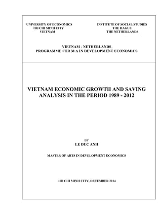
32. 26
Chapter 4: Empirical Analysis
In Chapter 4, the study presents estimated results for the interaction between economic
growth and saving with the confirmation of FDI in Vietnam. Step by step while
analyzing the 1989-2012 data, specific problems are solved and discussed as the
followings.
4.1 Empirical evidence
In this part, the study will employ the econometric techniques mentioned briefly at
Chapter 3 in which results of unit root test, ARDL cointegration bound test, long-run
coefficient estimation and VECM conditional on ARDL are presented respectively.
4.1.1 Unit root test results
The three variables are plotted on the graph as shown on Figure 1 below. There exists a
deterministic trend inside each series. Therefore, ADF and PP tests employed to detect
a problem of unit root existence should have a trend factor in unit-root test equations.
Figure 2: The graph of LGDP, LGDS and LFDI series
2
3
4
5
6
7
16
18
20
22
24
90 92 94 96 98 00 02 04 06 08 10 12
LFDI LGDP LGDS

33. 27
In detail, we could see that LFDI is said to be stationary at level by both unit root test
methods as shown on Table 2. Inversely, LGDP and LGDS are not stationary at level,
even the significance level is 10 per cent. Detecting orders of stationary in time series
analysis is the most important step because it will influence which method should be
employed to estimate short-run and long run effects amongst variables of interest.
Then, the next step is to check whether LGDP and LGDS are stationary at level 1 or
not.
Table 2: Unit root test of variables at level value
Variable
ADF PP
τ τ
log(GDP) -3.01 -1.62
log(GDS) -2.49 -3.13
log (FDI) -9.31***
-7.43***
Notes: the subscript τ in the model allows for a drift and deterministic trend. These (*),
(**) and (***) indicate the rejection of null hypothesis at 10 per cent, 5 per cent and 1
per cent respectively. Additionally, critical value obtains from MacKinnon (1995)
After taking the first difference of LGDP and LGDS, applying ADF and PP test, the
results in Table 3 show information as expected that two series are stationary at the
first difference. As Asteriou (2007) states most of economic indicators are trended,
therefore, rarely they are stationary at level data and usually stationary after taking the
first difference, and our research data is the case as he mentioned. For the case of
LGDS, the null hypothesis of non-stationary is rejected by two methods, thus this
series is said to be stationary at the first difference.

34. 28
Table 3: Unit root test of variables at the first difference
Variable
ADF PP
τ Μ τ Μ
ΔLGDP -4.03**
-2.64*
-2.96 -2.74*
ΔLGDS -3.92**
-5.13***
-6.39***
-5.09***
Notes: the subscript τ in the model allows for a drift and deterministic trend while μ
allowing for a drift. These (*), (**) and (***) indicate the rejection of null hypothesis
at 10 per cent, 5 per cent and 1 per cent respectively. Additionally, critical value
obtains from MacKinnon (1991)
Last but not the least, for the case of unit root tests of LGDP, PP test seems to fail to
reject the null hypothesis of non-stationary at the significance level 5 per cent. Then,
we must test on an assumption of ADF in which error term series of this test whether
follows the normal distribution or not. As shown at Appendix A.1, this error term
series follows a normal distribution, therefore, the results of ADF test for LGDP are
robust. Then, we could conclude that LGDS and LGDP are stationary at level 1, and
LFDI is stationary at level 0. Finally, ARDL method should be applied to test a
cointegration existence amongst these variables.
4.1.2 Cointegration test results
Based on the results of unit-root test, Johansen cointegration test for multivariate
causality could not be applied because this method only works if all relevant variables
are stationary at the same level. Therefore, ARDL bound test should be employed
instead of Johansen method. As mentioned in Chapter 3, ARDL is also effective in the
case of finite short time span. This is really important when analyzing Vietnam’s data
because the time span could not be longer the period 1989 – 2012 for three variables of
interest.
Tải bản FULL (76 trang): https://bit.ly/3h9DmHf
Dự phòng: fb.com/TaiHo123doc.net

35. 29
Table 4: Results of ARDL bound test
Dependent variable Independent
variables
Lag F-
statistic
Result
Equation
5
LGDS LGDP, LFDI 1 8.61 Cointegration
Equation
6
LGDP LGDS, LFDI 1 0.38 No cointegration
Equation
7
LFDI LGDS, LGDP 2 3.82 No cointegration
Lower-bound critical value for “without intercept and trend” at 1% = 3.88
Upper-bound critical value for “without intercept and trend” at 1% = 5.30
Applying the ARDL cointegration tests, we estimate three cointegration equations 5 –
7 as shown in Chapter 3. The maximum of lag length is 2 because the time span of
Vietnam data set is short, only 24 years, or on the other hand we have only 24
observations. Reducing the lag length of the first-difference terms corresponding to
each variable in each equation step by step, then we receive the optimum lag length is 1
based on Akaike information criterion for equations 5 to 6, but equation 7 with the
optimum lag length is 2 (see at Appendix A.2). the F statistical values are calculated
for the joint hypothesis of coefficients of lagged level terms in each equation
respectively given in Table 4. Comparing these statistical values with critical ones
given in the research by Pesaran (2001), we could only reject the null hypothesis of no
cointegration in equation 5. That means there is an existence of cointegration direction
from LGDP and LFDI to LGDS. Nevertheless, in equation 6 to 7, statistical values are
less than the lower-bound critical value, thus we accept the null hypothesis of no
cointegration.
Tải bản FULL (76 trang): https://bit.ly/3h9DmHf
Dự phòng: fb.com/TaiHo123doc.net

36. 30
4.1.3 Granger causality test results
The next step of ARDL bound test is to estimate a long run coefficient equation in the
form of equation 8. Detecting the optimum lag length based on Akaike information
criterion as the same way when estimating ARDL cointegration equations 5 – 7 (see at
Appendix A.3), finally ARDL (2, 0, 0) is employed to estimate long run coefficients
between LGDS, LGDP and LFDI. The results of long run coefficient equation are
shown on Table 5. As we could see, in long run LGDP really causes and pushes LGDS
represented by the coefficient value equals to 1.06 and is significant at 1 per cent.
Inversely LFDI causes, but tends to reduce LGDS represented by the coefficient value
equals to -0.12 and is significant at 5 percent.
Table 5: Estimated long run coefficients using the conditional ARDL(2, 0, 0)
Equation 8: LGDS is dependent variable
Variable Coefficient t-Statistic Probability
C -0.95 -0.74 0.47
LGDS(-1) 0.33 3.24 0.00
LGDS(-2) 0.04 0.43 0.67
LGDP 1.06 5.52 0.00
LFDI -0.12 -2.09 0.05
R2
= 0.97
Durbin-Watson Stat =2.06
F-statistic p-value = 0.00
In the causality analysis, estimating the long run adjustment coefficient 𝛼 is the most
important because it shows how strong the nexus amongst variables is. Based on the
long run coefficient equation estimated in form of equation 8 above, we receive the
error-term series (denoted as ECT – Error Correction Term) used to estimate the
adjustment coefficient. As mentioned above, we should estimate the short run

37. 31
coefficients combined with error terms. Then the VECM is applied in form of equation
11 because only this equation has the cointegration vector. The optimum lag length is
detected through estimating Unrestricted VAR amongst ΔLGDP, ΔLGDS and ΔLFDI
series. Then the optimum lag length 0 is selected by AIC (see more at Appendix A.3).
With the VECM results shown on Table 6, the long run adjustment coefficient (α)
equals to -0.706 and is significant at 5 per cent. It means there is an existence of long
run causal direction running from LGDP and LFDI to LGDS as early proved by the
ARDL bound test results above. The α value is -0.706 means the speed of adjustment
to equilibrium after an economic shock is high. Approximately 70.6% of
disequilibrium from the previous year’s shock could converge back to the long run
equilibrium in the current year (Asteriou, 2007).
Table 6: Results of VECM based on error terms taken from the conditional ARDL
VECM in a form of Equation 11: ΔLGDS is dependent variable
Variable Coefficient t-statistic Probability
C 0.001 0.008 0.993
ΔLGDP 2.068 0.678 0.507
ΔLFDI -0.105 -0.916 0.372
ECM(-1) -0.706 -2.184 0.043
R-squared = 0.277 0.277
Durbin-Watson
stat
1.499
Furthermore, this equation also passes all diagnostic tests including Ramsey RESET
test, White Heteroskedasticity test, Breusch-Godfrey Serial Correlation test and Jarque-
Berra Statistic for normality at the significant level 1 per cent. Furthermore, the results
of CUMSUM and CUMSUM-Squared tests (see more at Appendix A.3) show the
estimated coefficients and variance of VECM are stable in the period 1989 – 2012, on
6670216