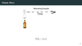
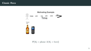
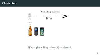
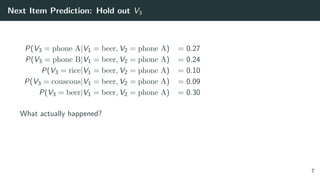
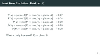
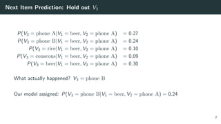
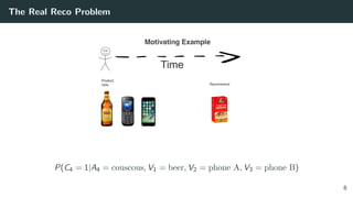
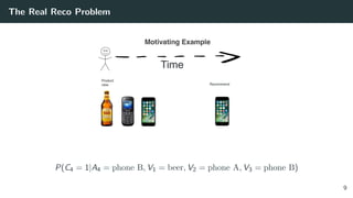
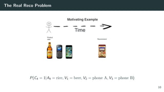
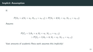
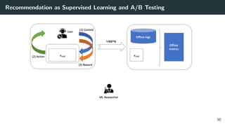
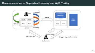
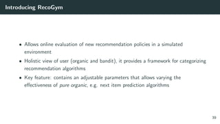
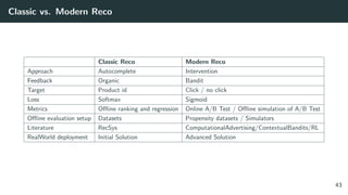
The document discusses the differences between classic and modern recommendation approaches. Classic recommendation frames the problem as next item prediction based on past user behavior, while modern recommendation frames it as predicting the success of intervention policies. Modern approaches aim to directly optimize business metrics and allow for better offline evaluation methods like inverse propensity scoring that can predict A/B test results. The document also outlines the experimentation lifecycle of real-world recommendation systems, which involves supervised learning from past user data, offline evaluation, A/B testing, and continuous improvement.

1. Modern Recommendation for Advanced Practitioners
Part I. Recommendation via Reward Modeling
Authors: Flavian Vasile, David Rohde, Amine Benhalloum, Martin Bompaire
Olivier Jeunen & Dmytro Mykhaylov
December 6, 2019

2. Acknowledgments
Special thanks to our colleagues, both from Criteo and academia, that contributed to
RecoGym and to some of the methods covered: Stephen Bonner, Alexandros
Karatzoglou, Travis Dunlop, Elvis Dohmatob, Louis Faury, Ugo Tanielian, Alexandre
Gilotte
1

3. Course
• Part I. Recommendation via Reward Modeling
• I.1. Classic vs. Modern: Recommendation as Autocomplete vs. Recommendation as
Intervention Policy
• I.2. Recommendation Reward Modeling via (Point Estimation) Maximum Likelihood
Models
• I.3. Shortcomings of Classical Value-based Recommendations
• Part II. Recommendation as Policy Learning Approaches
• II.1. Policy Learning: Concepts and Notations
• II.2. Fixing the issues of Value-based Models using Policy Learning
• Fixing Covariate Shift using Counterfactual Risk Minimization
• Fixing Optimizer’s Curse using Distributional Robust Optimization
• II.3. Recap and Conclusions
2

4. Getting Started with RecoGym and Google Colaboratory
• Open your favorite browser and go to the course repository:
https://github.com/criteo-research/bandit-reco
• You will find the notebooks and the slides for the course
• You can access the notebooks directly on Google Collab in the following manner:
- https://colab.research.google.com/github/criteo-research/
bandit-reco/blob/master/notebooks/0.%20Getting%20Started.ipynb
• Alternatively, clone the repository and run the notebooks locally.
• . . . you’re all set!
3

5. Part I. Recommendation via
Reward Modeling
3

6. I.1. Classic vs. Modern:
Recommendation as
Autocomplete
vs.
Recommendation as
Intervention Policy

7. What Makes a Recommender System Modern?
3

8. Classic Reco
P(V1 = beer)
4

9. Classic Reco
P(V2 = phone A|V1 = beer)
5

10. Classic Reco
P(V3 = phone B|V1 = beer, V2 = phone A)
6

11. Next Item Prediction: Hold out V3
P(V3 = phone A|V1 = beer, V2 = phone A) = 0.27
P(V3 = phone B|V1 = beer, V2 = phone A) = 0.24
P(V3 = rice|V1 = beer, V2 = phone A) = 0.10
P(V3 = couscous|V1 = beer, V2 = phone A) = 0.09
P(V3 = beer|V1 = beer, V2 = phone A) = 0.30
What actually happened?
7

12. Next Item Prediction: Hold out V3
P(V3 = phone A|V1 = beer, V2 = phone A) = 0.27
P(V3 = phone B|V1 = beer, V2 = phone A) = 0.24
P(V3 = rice|V1 = beer, V2 = phone A) = 0.10
P(V3 = couscous|V1 = beer, V2 = phone A) = 0.09
P(V3 = beer|V1 = beer, V2 = phone A) = 0.30
What actually happened? V3 = phone B
7

13. Next Item Prediction: Hold out V3
P(V3 = phone A|V1 = beer, V2 = phone A) = 0.27
P(V3 = phone B|V1 = beer, V2 = phone A) = 0.24
P(V3 = rice|V1 = beer, V2 = phone A) = 0.10
P(V3 = couscous|V1 = beer, V2 = phone A) = 0.09
P(V3 = beer|V1 = beer, V2 = phone A) = 0.30
What actually happened? V3 = phone B
Our model assigned: P(V3 = phone B|V1 = beer, V2 = phone A) = 0.24
7

14. The Real Reco Problem
P(C4 = 1|A4 = couscous, V1 = beer, V2 = phone A, V3 = phone B)
8

15. The Real Reco Problem
P(C4 = 1|A4 = phone B, V1 = beer, V2 = phone A, V3 = phone B)
9

16. The Real Reco Problem
P(C4 = 1|A4 = rice, V1 = beer, V2 = phone A, V3 = phone B)
10

17. What we have vs. what we want
Our model:
P(V4 = phone A|V1 = beer, V2 = phone A, V3 = phone A) = 0.27
P(V4 = phone B|V1 = beer, V2 = phone A, V3 = phone A) = 0.28
P(V4 = rice|V1 = beer, V2 = phone A, V3 = phone A) = 0.12
P(V4 = couscous|V1 = beer, V2 = phone A, V3 = phone A) = 0.14
P(V4 = beer|V1 = beer, V2 = phone A, V3 = phone A) = 0.19
Which is a vector of size P that sums to 1.
We want:
11

18. What we have vs. what we want
Our model:
P(V4 = phone A|V1 = beer, V2 = phone A, V3 = phone A) = 0.27
P(V4 = phone B|V1 = beer, V2 = phone A, V3 = phone A) = 0.28
P(V4 = rice|V1 = beer, V2 = phone A, V3 = phone A) = 0.12
P(V4 = couscous|V1 = beer, V2 = phone A, V3 = phone A) = 0.14
P(V4 = beer|V1 = beer, V2 = phone A, V3 = phone A) = 0.19
Which is a vector of size P that sums to 1.
We want:
P(C4 = 1|A4 = phone A, V1 = beer, V2 = phone A, V3 = phone A) = ?
P(C4 = 1|A4 = phone B, V1 = beer, V2 = phone A, V3 = phone A) = ?
P(C4 = 1|A4 = rice, V1 = beer, V2 = phone A, V3 = phone A) = ?
P(C4 = 1|A4 = couscous, V1 = beer, V2 = phone A, V3 = phone A) = ?
P(C4 = 1|A4 = beer, V1 = beer, V2 = phone A, V3 = phone A) = ?
Which is a vector of size P where each entry is between 0 and 1. 11

19. Implicit Assumption
Our model predicts:
P(V4 = phone A|V1 = beer, V2 = phone A, V3 = phone A) = 0.27
P(V4 = phone B|V1 = beer, V2 = phone A, V3 = phone A) = 0.28
P(V4 = rice|V1 = beer, V2 = phone A, V3 = phone A) = 0.12
P(V4 = couscous|V1 = beer, V2 = phone A, V3 = phone A) = 0.14
P(V4 = beer|V1 = beer, V2 = phone A, V3 = phone A) = 0.19
So let’s recommend phone B, it has the highest next item probability.
12

20. Implicit Assumption
If:
P(Vn = a|V1 = v1..Vn−1 = vn−1) > P(Vn = b|V1 = v1..Vn−1 = vn−1)
Assume:
P(Cn = 1|An = a, V1 = v1..Vn−1 = vn−1)
> P(Cn = 1|An = b, V1 = v1..Vn−1 = vn−1)
Vast amounts of academic Reco work assumes this implicitly!
13

21. Classical vs. Modern Recommendation
• Classical Approach: Recommendation as Autocomplete:
• Typically leverage organic user behaviour information (e.g. item views, page visits)
• Frame the problem either as missing link prediction/MF problem, either as a next
event prediction, sequence prediction problem
• Modern Approach: Recommendation as Intervention Policy:
• Typically leverage bandit user behaviour information (e.g. ad clicks)
• Frame the problem either as click likelihood problem, either as a contextual
bandit/policy learning problem
14

22. I.1.1. Advantages of the Classical
Approach

23. Academia
• An already established framework
• Standard datasets and metrics
• Easier to publish and compare methods!
15

24. Real-World
• Data arises naturally from the use of the application (before any recommendation
system in place)
• Methods have standard efficient and well-tested implementations
• Very good initial system!
16

25. I.1.2. Limitations of the Classical
Approach

26. What is Wrong with the Classical Formulation?
We are operating under the assumption that the best recommendation policy is, in
some sense, the optimal auto-complete of natural user behavior.
17

27. Solving the Wrong Problem
From the point of view of business metrics, learning to autocomplete behavior is a
great initial recommendation policy, especially when no prior user feedback is
available.
However, after a first golden age, where all offline improvements turn into positive
A/B tests, the naive recommendation optimization objective and the business objective
will start to diverge.
18

28. Solving the Wrong Problem: are the Classic Datasets Logs of RecSys?
• MovieLens: no, explicit feedback of movie ratings [1]
• Netflix Prize: no, explicit feedback of movie ratings [2]
• Yoochoose (RecSys competition ’15): no, implicit session-based behavior [3]
• 30 Music: no, implicit session-based behavior [4]
• Yahoo News Feed Dataset: yes! [5]
• Criteo Dataset for counterfactual evaluation of RecSys algorithms: yes! [6]
19

29. Solving the Wrong Problem: are the Classic Datasets Logs of RecSys?
• MovieLens: no, explicit feedback of movie ratings [1]
• Netflix Prize: no, explicit feedback of movie ratings [2]
• Yoochoose (RecSys competition ’15): no, implicit session-based behavior [3]
• 30 Music: no, implicit session-based behavior [4]
• Yahoo News Feed Dataset: yes! [5]
• Criteo Dataset for counterfactual evaluation of RecSys algorithms: yes! [6]
The Criteo Dataset shows a log of recommendations and if they were successful in
getting users to click.
19

30. Solving the Wrong Problem: do the Classical Offline Metrics Evaluate the Qual-
ity of Recommendation?
Classical offline metrics:
• Recall@K, Precision@K, HR@K: How often is an item in the top k - no, evaluates
next item prediction
• DCG: Are we assigning a high score to an item - no, evaluates next item prediction
Online metrics and their offline simulations:
• A/B Test: i.e. run a randomized control trial live — yes, but expensive + the
academic literature has no access to this
• Inverse Propensity Score estimate of click-through rate: - to be explained later.
— yes! (although it is often noisy) [7]
20

31. Solving the wrong problem: Do the classical offline metrics evaluate the quality
of recommendation?
Bottom line: If the dataset does not contain a log of recommendations, and if they
were successful, you cannot compute metrics of the recommendation quality!
21

32. I.1.3. Modern Reco: Solving the
Problems of Classical Approach

33. Aligning the Recommendation Objective with the Business Objectives
• Of course, we could start incorporating user feedback that we collected while
running the initial recommendation policies
• We should be able to continue bringing improvements using feedback that is now
aligned with our business metrics (ad CTR, post-click sales, dwell time, number of
videos watched, ...)
22

34. Better Offline Evaluation
22

35. Offline Evaluation that Predicts an A/B Test Result
Let’s follow the previous notation (A action/recommended item, V organic item
view/interaction) and denote π the recommendation policy (that assign probabilities to
items conditionally on user past).
23

36. Offline Evaluation that Predicts an A/B Test Result
Let’s follow the previous notation (A action/recommended item, V organic item
view/interaction) and denote π the recommendation policy (that assign probabilities to
items conditionally on user past). Imagine we have a new recommendation policy
πt(An = an|V1 = v1, ..., Vn = vn−1), can we predict how well it will perform if we
deploy it? We collected logs from a different policy:
π0(An = an|V1 = v1, ..., Vn = vn−1)
Let’s examine some hypothetical logs...
23

37. Offline Evaluation via IPS
Imagine the user clicks
πt(A4 = phone B|V1 = beer, V2 = phone A, V3 = phone B) = 1
π0(A4 = phone B|V1 = beer, V2 = phone A, V3 = phone B) = 0.8
The new policy will recommend “phone B” the 1
0.8 = 1.25× as often as the old policy.
24

38. Offline Evaluation via IPS
Imagine the user clicks
πt(A2 = rice|V1 = couscous) = 1
π0(A2 = rice|V1 = couscous) = 0.01
The new policy will recommend “rice” the 1
0.01 = 100× as often as the old policy.
25

39. Offline Evaluation IPS
Let’s denote cn the feedback on the nth recommendation, i.e. 1 if the recommendation
got clicked else 0.
26

40. Offline Evaluation IPS
Let’s denote cn the feedback on the nth recommendation, i.e. 1 if the recommendation
got clicked else 0.
Let’s re-weight each click by how much more likely the recommendation will appear
under the new policy πt compared the logging policy π0)
26

41. Offline Evaluation IPS
Let’s denote cn the feedback on the nth recommendation, i.e. 1 if the recommendation
got clicked else 0.
Let’s re-weight each click by how much more likely the recommendation will appear
under the new policy πt compared the logging policy π0)
We will assume that X = f (v1, ..., vn). Crafting f (·) is often called “feature
engineering”.
CTR estimate = Eπ0
c · πt(a|X)
π0(a|X)
≈
1
N
N
n
cnπt (a|X)
π0 (an|X)
26

42. Offline Evaluation via IPS
This estimator is unbiased
CTR estimate = Eπ0
c · πt(a|X)
π0(a|X)
= Eπt [c]
27

43. Offline Evaluation via IPS
Shortcomings:
• We only look at the clicks i.e. cn = 1 (otherwise the contribution is 0).
• When the new policy differs markedly from the old, the weights become very high
(to compensate for the fact that these are rare examples in your sample). These
rare high values contribute a lot to the variance of the estimator.
28

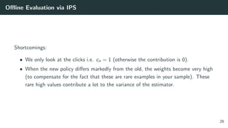
44. Offline Evaluation via IPS
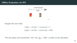
Overall, IPS actually attempts to answer a counterfactual question (what would have
happened if instead of π0 we would have used πt ?), but it often has less than
spectacular results because of its variance issues.
A lot of the shortcomings of the naive IPS estimator are handled in [8].
29

45. The Experimentation Life-Cycle of Real-World
Recommendation Systems
29

46. Recommendation as Supervised Learning and A/B Testing
30

47. Recommendation as Supervised Learning and A/B Testing
31

48. Recommendation as Supervised Learning and A/B Testing
32

49. Recommendation as Supervised Learning and A/B Testing
33

50. Recommendation as Supervised Learning and A/B Testing
34

51. Let’s Take a Step Back...
How are we improving large-scale Recommender Systems in the Real World
• Learn a supervised model from past user activity
• Evaluate offline and decide whether to A/B test
• A/B test
• If positive and scalable, roll-out
• If not, try to understand what happened and try to create a better model of the
world using the same past data
• Repeat
35

52. Relationship Between Reinforcement Learning and Recommendation
• We are doing Reinforcement Learning by hand!
• Furthermore, we are trying to do RL using the Supervised Learning Framework
• Standard test data sets do not let us explore this aspect of recommender systems
.. but how do you evaluate offline a reinforcement learning algorithm?
36

53. 1.4. RecoGym: an Offline Simulator
for Recommendation

54. OpenAI Gym
• Problem: The reinforcement learning community lacked a common set of tools to
allow comparison of reinforcement learning algorithms.
• OpenAI Gym: Software standard (Python API) that allows comparions of the
performance of reinforcement learning algorithms
• Core idea: Environments define the problem and the agents (the RL algorithms)
try to solve it by repeated interactions.
37

55. Introducing RecoGym
RecoGym: An OpenAI compatible environment that simulates user behavior (both
organic and bandit, e.g. its reaction to recommendation agents)
38

56. Introducing RecoGym
• Allows online evaluation of new recommendation policies in a simulated
environment
• Holistic view of user (organic and bandit), it provides a framework for categorizing
recommendation algorithms
• Key feature: contains an adjustable parameters that allows varying the
effectiveness of pure organic, e.g. next item prediction algorithms
39

57. The Simulation Model for Organic and Bandit Feedback
40

58. Let’s Get Started
An introductory notebook to RecoGym can be found: click here!
We will be using Google Colab, so you have nothing to install!
41

59. Exercise no. I.1: Organic Best Of
vs. Bandit Best Of

60. Exercise - The best of the best
Go to the notebook 1. Organic vs Bandit Best Ofs (click here)
• Examine the logs; to start with, we will look at non-personalized behavior only.
• Plot a histogram of organic product popularity. What is the most popular
product?
• Plot the (non-personalized) click-through rate of each product (with an error
analysis). What is the most clicked-on product?
• Plot popularity against click-through rate. How good is proxy popularity for
click-through rate?
• Simulate an A/B test comparing a simple recommender system (agent) that
always recommends the highest CTR product with a recommender system that
always recommends the organically most popular product.
42

61. A quick recap of the differences
between classic and modern reco

62. Classic vs. Modern Reco
Classic Reco Modern Reco
Approach Autocomplete Intervention
Feedback Organic Bandit
Target Product id Click / no click
Loss Softmax Sigmoid
Metrics Offline ranking and regression Online A/B Test / Offline simulation of A/B Test
Offline evaluation setup Datasets Propensity datasets / Simulators
Literature RecSys ComputationalAdvertising/ContextualBandits/RL
RealWorld deployment Initial Solution Advanced Solution
43

63. I.2. Recommendation Reward
Modeling via (Point
Estimation) Maximum
Likelihood Models

64. Maximum Likelihood-based Agent
How can we build an agent/recommender from historical recommendation data i.e.
(Xn, an, cn) ?
44

65. Maximum Likelihood-based Agent
How can we build an agent/recommender from historical recommendation data i.e.
(Xn, an, cn) ?
The most straight-forward way is to first frame the task as a reward/click prediction
task.
44

66. Maximum Likelihood-based Agent
How can we build an agent/recommender from historical recommendation data i.e.
(Xn, an, cn) ?
The most straight-forward way is to first frame the task as a reward/click prediction
task.
The classical solution:
Maximum Likelihood Linear Model = Logistic Regression
44

67. Maximum Likelihood-based Agent
How can we build an agent/recommender from historical recommendation data i.e.
(Xn, an, cn) ?
The most straight-forward way is to first frame the task as a reward/click prediction
task.
The classical solution:
Maximum Likelihood Linear Model = Logistic Regression
Point estimation = Estimates the best fit solution only = Non-Bayesian Model
44

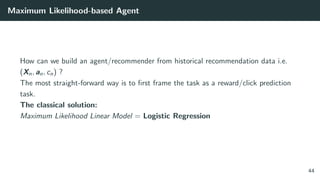
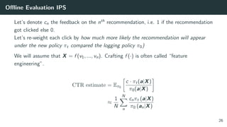
68. Reward(Click) Modeling via Logistic Regression
cn ∼ Bernoulli σ Φ([Xn an])T
β
where
• X represent context or user features
• a represent action or product features
• β are the parameters;
• σ (·) is the logistic sigmoid;
• Φ (·) is a function that maps X, a to a higher dimensional space and includes
some interaction terms between Xn and an.
45

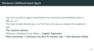
69. Reward(Click) Modeling via Logistic Regression
cn ∼ Bernoulli σ Φ([Xn an])T
β
where
• X represent context or user features
• a represent action or product features
• β are the parameters;
• σ (·) is the logistic sigmoid;
• Φ (·) is a function that maps X, a to a higher dimensional space and includes
some interaction terms between Xn and an. Why?
45

70. Modeling interaction between user/context and product/action
• Φ ([Xn an]) = Xn ⊗ an Kronecker product, this is somewhat what we will be
doing in the example notebook, these will model pairwise interactions between
user and product features.
• Φ ([Xn an]) = ν(Xn) · µ(an) Another more ”modern” approach, is to build an
embedded representation of the user and product features and consider the dot
product between both (in this case the parameters of the model are carried in the
embedding functions ν and µ and we have no parameter vector β)
46

71. Reward(Click) Modeling via Logistic Regression
Then it’s just a classification problem, right? We want to maximize the log-likelihood:
ˆβlh = argmaxβ
n
cn log σ Φ ([Xn an]))T
β
+ (1 − cn) log 1 − σ Φ ([Xn an])T
β
47

72. Other Possible Tasks
Imagine we recommend a group of items (a banner with products, for instance), and
one of them gets clicked, an appropriate task would be to rank the clicked items higher
than non clicked items.
Example: Pairwise Ranking Loss
n
log σ Φ ([Xn an])T
β − Φ Xn a n
T
β
Where an represent a clicked item from group n and a n a non clicked item.
Multitude of possible other tasks (list-wise ranking, top-1, ...) e.g. BPR [9]
48

73. I.2.1. Using Reward Models to Act

74. Value-based Models for Recommendation
To choose which action to take, we need to evaluate all possible actions and take the
one maximizing the predicted reward.
This is a value-based model approach to Recommendation, where in order to take the
optimal action we:
49

75. Value-based Models for Recommendation
To choose which action to take, we need to evaluate all possible actions and take the
one maximizing the predicted reward.
This is a value-based model approach to Recommendation, where in order to take the
optimal action we:
• Step1: Build a value model that can estimate the reward of using any action in
the context of any user
49

76. Value-based Models for Recommendation
To choose which action to take, we need to evaluate all possible actions and take the
one maximizing the predicted reward.
This is a value-based model approach to Recommendation, where in order to take the
optimal action we:
• Step1: Build a value model that can estimate the reward of using any action in
the context of any user
• Step2: At decision time, evaluate all possible actions given the user context
49

77. Max.Likelihood Model → Recommendation Policy
In the LR case, our max likelihood click predictor can be converted into a
(deterministic) policy by just taking the action with the highest predicted click
probability.
50

78. Sidepoint: Scaling argmax in the Case of Large Action Spaces
• Imagine we mapped the context/user features X into a dense representation
(embedding) u
• Same thing for the action/product features a into v
• Such that P(c = 1|X, a) = σ (u · v)
• Choosing for a given context the reward maximizing action is a Maximum
InnerProduct Search (MIPS) problem, which is a very well studied problem for
which approximate solutions have a high quality
51

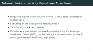
79. Sidepoint: Scaling argmax in the Case of Large Action Spaces
• Several method families
• Hashing based: Locality Sensitive Hashing [10]
• Tree based: Random Projection Trees [11]
• Graph based: Navigable Small World Graphs [12]
• Bottom line: use and abuse them!
52

80. Exercise no. I.2: Pure Bandit Model

81. Pure Bandit Feedback
• Build a model using feature engineering using logistic regression (or a deep model)
53

82. Pure Bandit Feedback
• Build a model using feature engineering using logistic regression (or a deep model)
• Finally you evaluate your performance against production.
53

83. Pure Bandit Feedback
• Build a model using feature engineering using logistic regression (or a deep model)
• Finally you evaluate your performance against production.
Please look at notebook “2. Likelihood Agent.ipynb” Click here!
53

84. I.3. Shortcomings of Classical
Value-based
Recommendations

85. I.3.1. Covariate Shift Problem

86. Issue #1: The Covariate Shift Problem
The problem: We train our value model on one distribution of (reward,
context, action) tuples, but we test on another!
• Train on: P(c = 1|X, a) · π0(a|X) · P(X)
• (Online) test on: P(c = 1|X, a) · πunif(a|X) · P(X)
In the case of value based recommendations we are biased at training time (because of
the logging policy) but we are always evaluating on the uniform distribution (because
of the argmax).
54

87. Good Recommendations are Similar to History, but not too Similar
55

88. Historical Reco Tries to be Good, It is Mostly Very Similar to History
56

89. When we Evaluate New Actions we do this Uniformly. The Model Underfits
Badly where most of the Data are
57

90. A Re-weighting Scheme Makes the Underfit Uniform when we Evaluate
58

91. Covariate Shift and Model Misspecification
Covariate Shift and Model Underfitting
• If we have a perfect predictor for P(c = 1|X, a), why should we care if π(a|X)
changes?
• Of course, P(c = 1|X, a) is not perfect and it is usually designed to underfit (to
insure generalization through capacity constraints — limited degrees of freedom)
• In this case, we should allocate the model capacity on the portions of the π(a|X)
where the model will be tested
59

92. Covariate Shift and Recommendation
• Note: In the case of using value-based models for decision making (and in our
case, Recommendation) we will evaluate all actions for all contexts so we will need
to be good everywhere!
In Part 2, we will see how we are going to solve this, but first let’s talk about the
second issue!
60

93. I.3.2. The Optimizer’s Curse

94. Issue #2: Optimizer’s Curse: a Story
61

95. Issue #2: Optimizer’s Curse: a Story
Day1: Offline Evaluation Time (Predicted Reward)
• Imagine a decision problem, handed to us by our CEO, where we need to choose
between 3 actions and where, for each one of them, we have samples of historical
rewards.
• In order to choose, we build empirical reward estimators for each of the 3 actions,
we find the one that has the best historical performance and we go back to our
CEO with the recommendation! After work, we congratulate ourselves and go to
sleep happy!
62

96. Issue #2: Optimizer’s Curse: a Story
Day2: Online Evaluation Time (True Reward)
• However, the next day we meet with the CEO only to find out this was just a test
of our decision-making capabilities, and that all of the sampled rewards for the 3
actions were all drawn independently from the same distribution.
• Due to the finite nature of our samples, each one of our 3 reward estimators made
errors, some of them more negative (pessimistic), and some of them more positive
(optimistic).
• Because when we decided, we selected the action with the highest estimate, we
obviously favored the most optimistic of the 3, making us believe we optimized
our decision, when we were just overfitting the historical returns. This effect is
known at the Optimizer’s Curse.
63

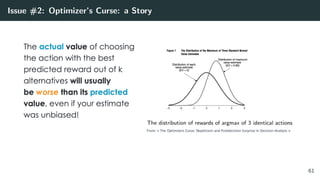
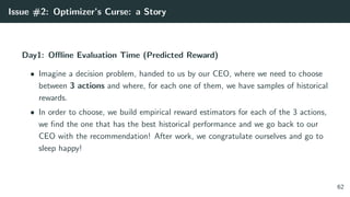
97. Issue #2: The Optimizer’s Curse. A Story
Figure 1: The distribution of rewards of argmax of 3 actions with ∆ separation. From: The
Optimizer’s Curse: Skepticism and Postdecision Surprise in Decision Analysis [13]
64

98. Optimizer’s Curse in Recommendation
• The Optimizer’s Curse mainly appears when the reward estimates are based on
small sample sizes and the deltas between the true mean rewards of the
different actions are relatively small such that the variance of the empirical
estimators can lead to overoptimistic expectations or even erroneous ranking of
actions.
• This is not a corner case! In real recommendation applications, the space of
possible context-action pairs is extremely large, so there are always areas of the
distribution where the current system is deciding based on very low sample sizes.
65

99. Fixing Covariate Shift and Optimizer’s Curse with Policy Learning
We saw that value-based approaches for decision-making suffer from two issues when
using ERM-based models.
In Part II. we will show how to solve both issues !
66

100. Example 3. Showcasing the
Optimizer’s Curse effect in our
likelihood agent

101. Demo: Expected CTR vs. Observed CTR
We will be using our likelihood model to showcase optimizer’s curse, where we
overstimate the number of clicks we will be getting from showing particular products.
The notebook is “3 Optimizer’s curse“ (Click here)
67

102. Wrapping-up Part I. of our course

103. What have we learnt so far?
• How the classical recommendation setting differs from real world recommendation
• Using a simulator aka RecoGym to build and evaluate recommender agents
• Shortcomings of value-based models with maximum likelihood estimators (e.g.
LR) (covariate shift and optimizer’s curse)
68

104. About Part II.
• Frame the problem in the contextual bandit vocabulary
• We will introduce an alternative approach to value-based models to solve the
covariate shift issue
• We will define a theoretical framework to help reason about Optimizer’s Curse
and solve the issue
69

105. Thank You!
69

106. Questions?
69

107. References i
References
[1] F Maxwell Harper and Joseph A Konstan. The movielens datasets: History and
context. Acm transactions on interactive intelligent systems (tiis), 5(4):19, 2016.
[2] James Bennett, Stan Lanning, et al. The netflix prize. In Proceedings of KDD
cup and workshop, volume 2007, page 35. New York, NY, USA., 2007.
[3] David Ben-Shimon, Alexander Tsikinovsky, Michael Friedmann, Bracha Shapira,
Lior Rokach, and Johannes Hoerle. Recsys challenge 2015 and the yoochoose
dataset. In Proceedings of the 9th ACM Conference on Recommender Systems,
pages 357–358. ACM, 2015.
70

108. References ii
[4] Roberto Turrin, Massimo Quadrana, Andrea Condorelli, Roberto Pagano, and
Paolo Cremonesi. 30music listening and playlists dataset. In RecSys 2015 Poster
Proceedings, 2015. Dataset: http://recsys.deib.polimi.it/datasets/.
[5] Yahoo. Yahoo news feed dataset, 2016.
[6] Damien Lefortier, Adith Swaminathan, Xiaotao Gu, Thorsten Joachims, and
Maarten de Rijke. Large-scale validation of counterfactual learning methods: A
test-bed. arXiv preprint arXiv:1612.00367, 2016.
[7] Daniel G Horvitz and Donovan J Thompson. A generalization of sampling
without replacement from a finite universe. Journal of the American statistical
Association, 47(260):663–685, 1952.
71

109. References iii
[8] Alexandre Gilotte, Cl´ement Calauz`enes, Thomas Nedelec, Alexandre Abraham,
and Simon Doll´e. Offline a/b testing for recommender systems. In Proceedings of
the Eleventh ACM International Conference on Web Search and Data Mining,
pages 198–206. ACM, 2018.
[9] Steffen Rendle, Christoph Freudenthaler, Zeno Gantner, and Lars
Schmidt-Thieme. Bpr: Bayesian personalized ranking from implicit feedback. In
Proceedings of the twenty-fifth conference on uncertainty in artificial intelligence,
pages 452–461. AUAI Press, 2009.
[10] Aristides Gionis, Piotr Indyk, Rajeev Motwani, et al. Similarity search in high
dimensions via hashing. In Vldb, volume 99, pages 518–529, 1999.
72

110. References iv
[11] erikbern. Approximate nearest neighbors in c++/python optimized for memory
usage and loading/saving to disk, 2019.
[12] Yury A Malkov and Dmitry A Yashunin. Efficient and robust approximate nearest
neighbor search using hierarchical navigable small world graphs. IEEE transactions
on pattern analysis and machine intelligence, 2018.
[13] James E Smith and Robert L Winkler. The optimizer’s curse: Skepticism and
postdecision surprise in decision analysis. Management Science, 52(3):311–322,
2006.
73