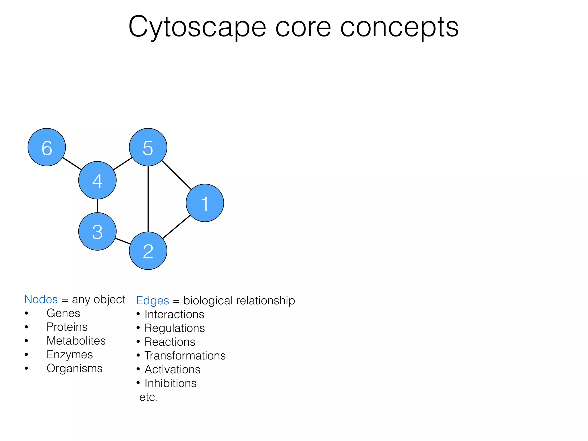
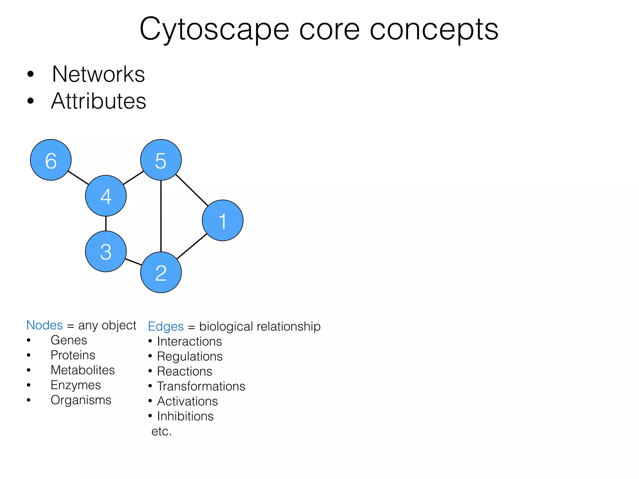
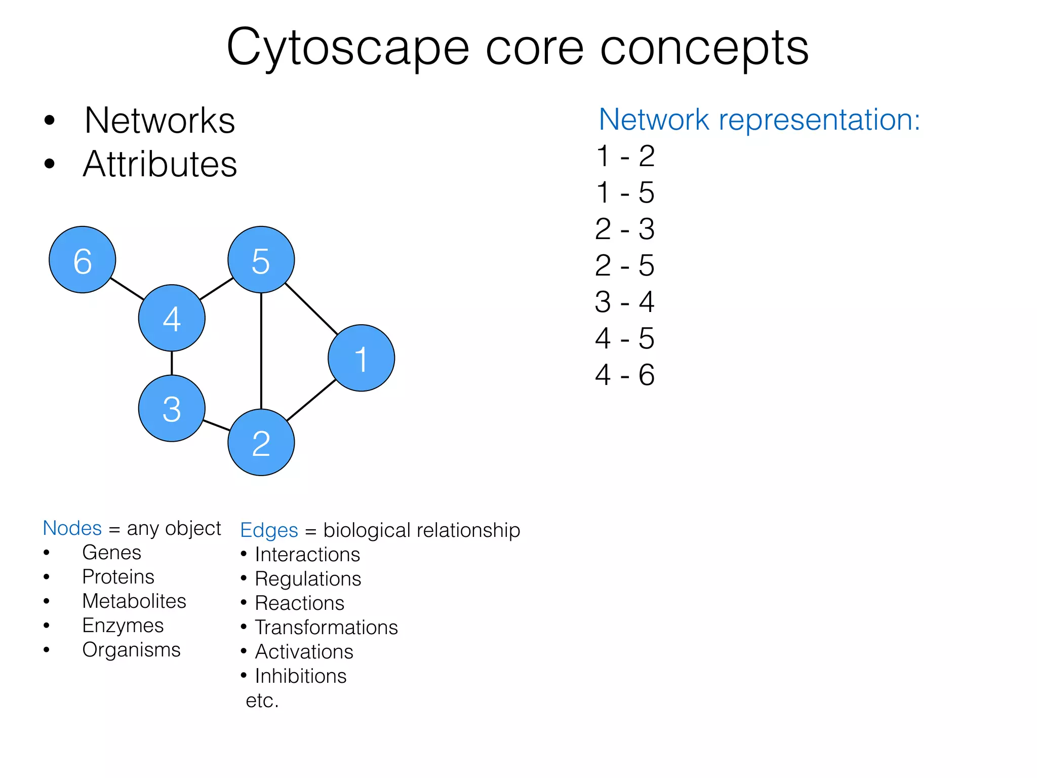
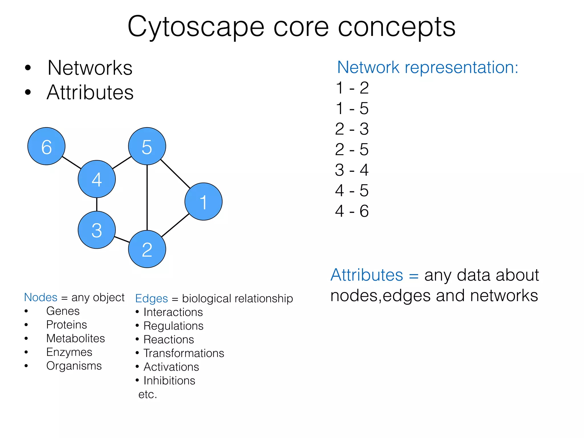
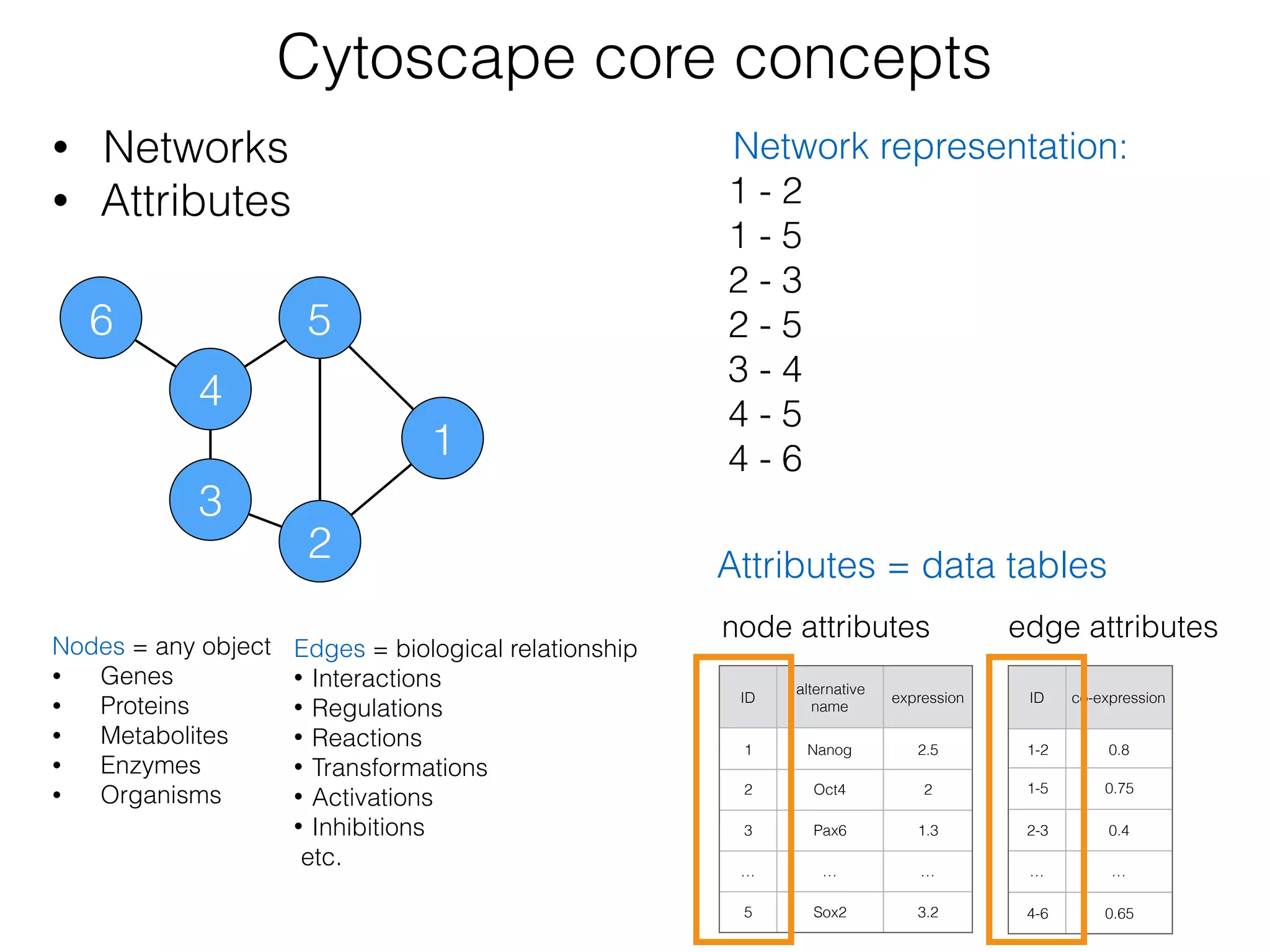
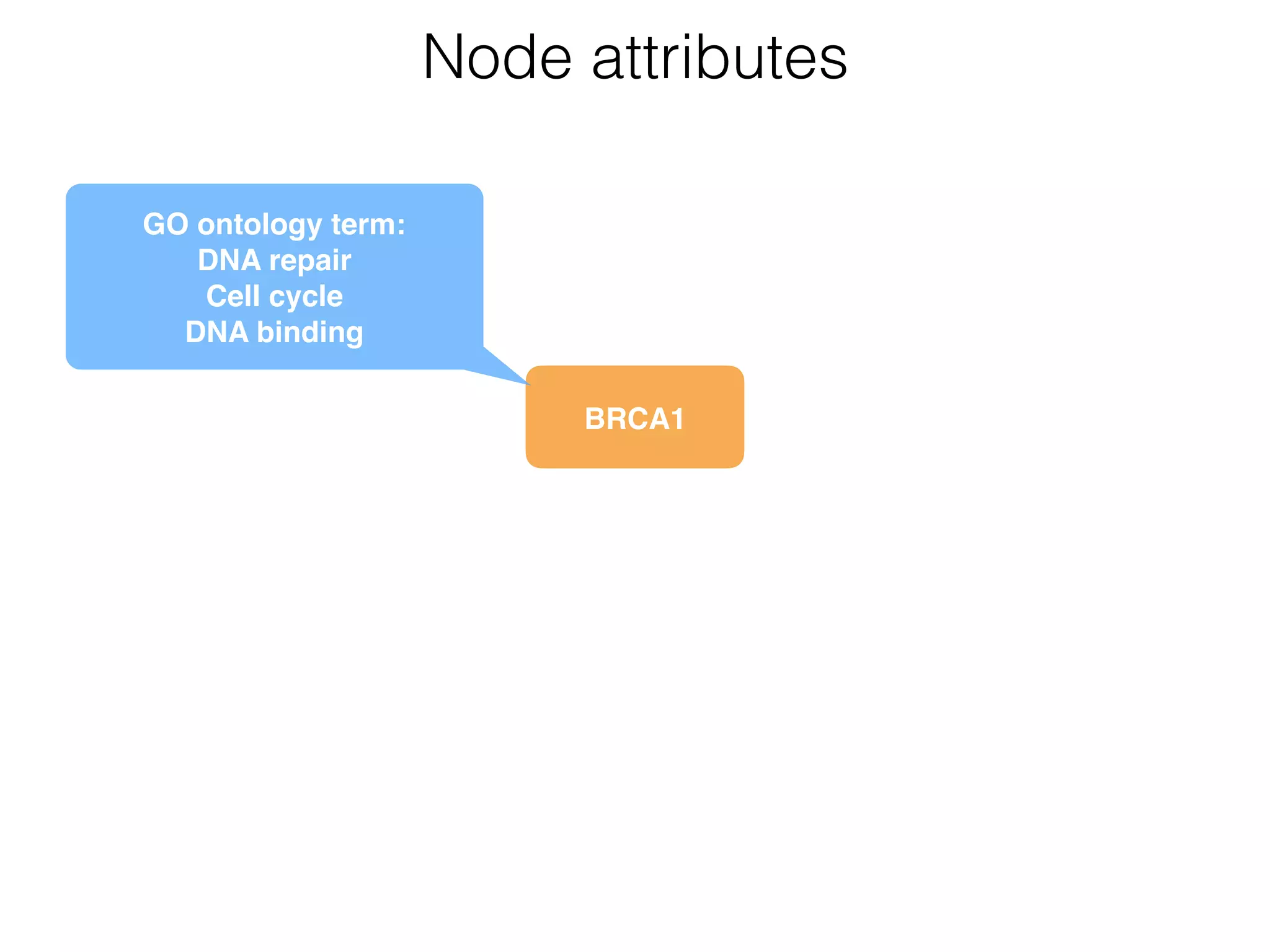
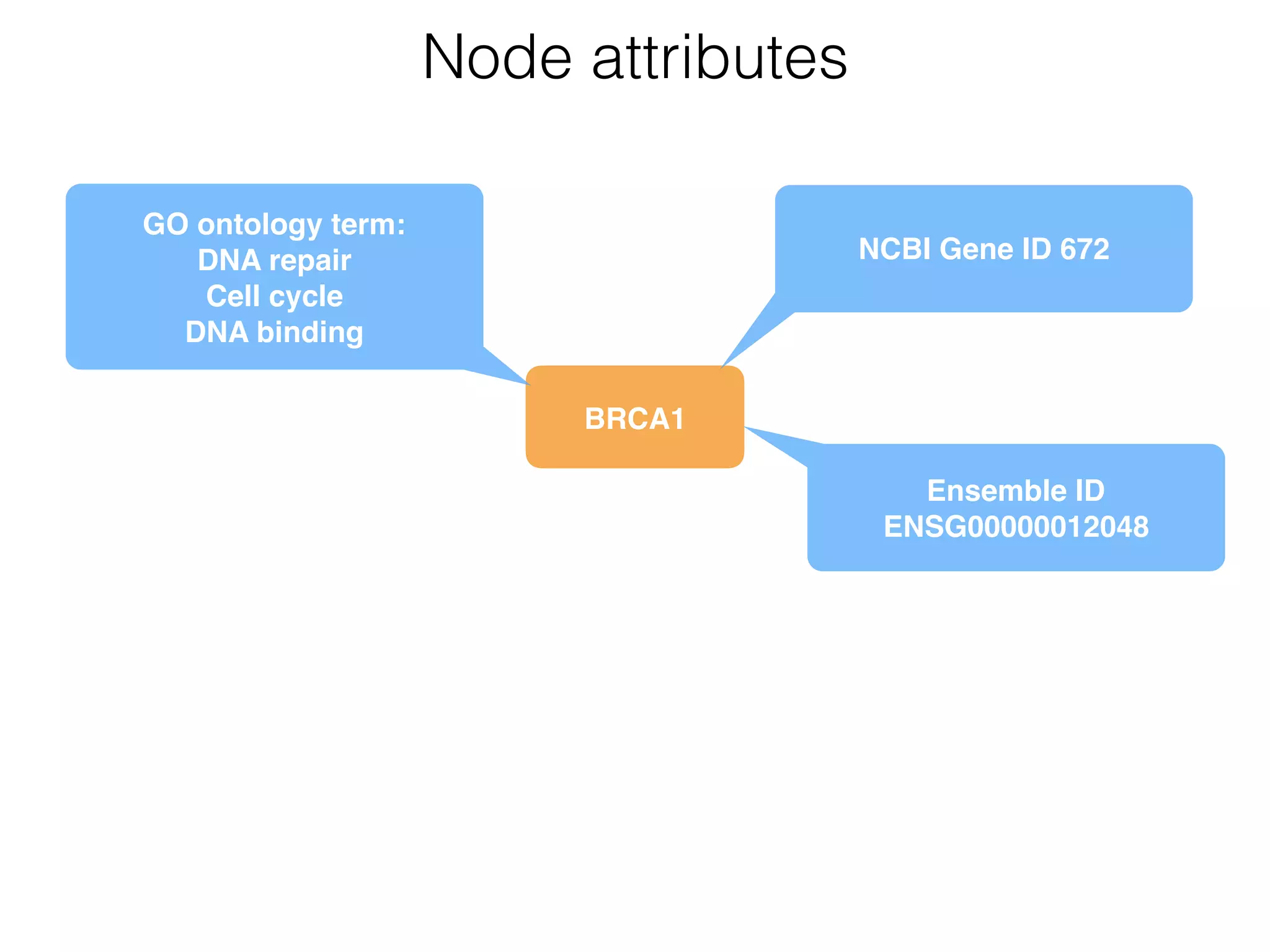
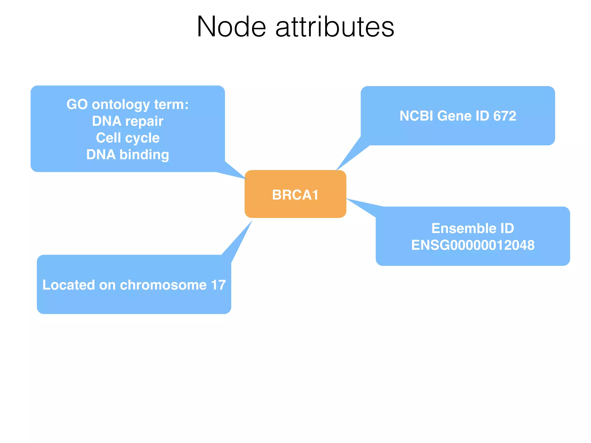
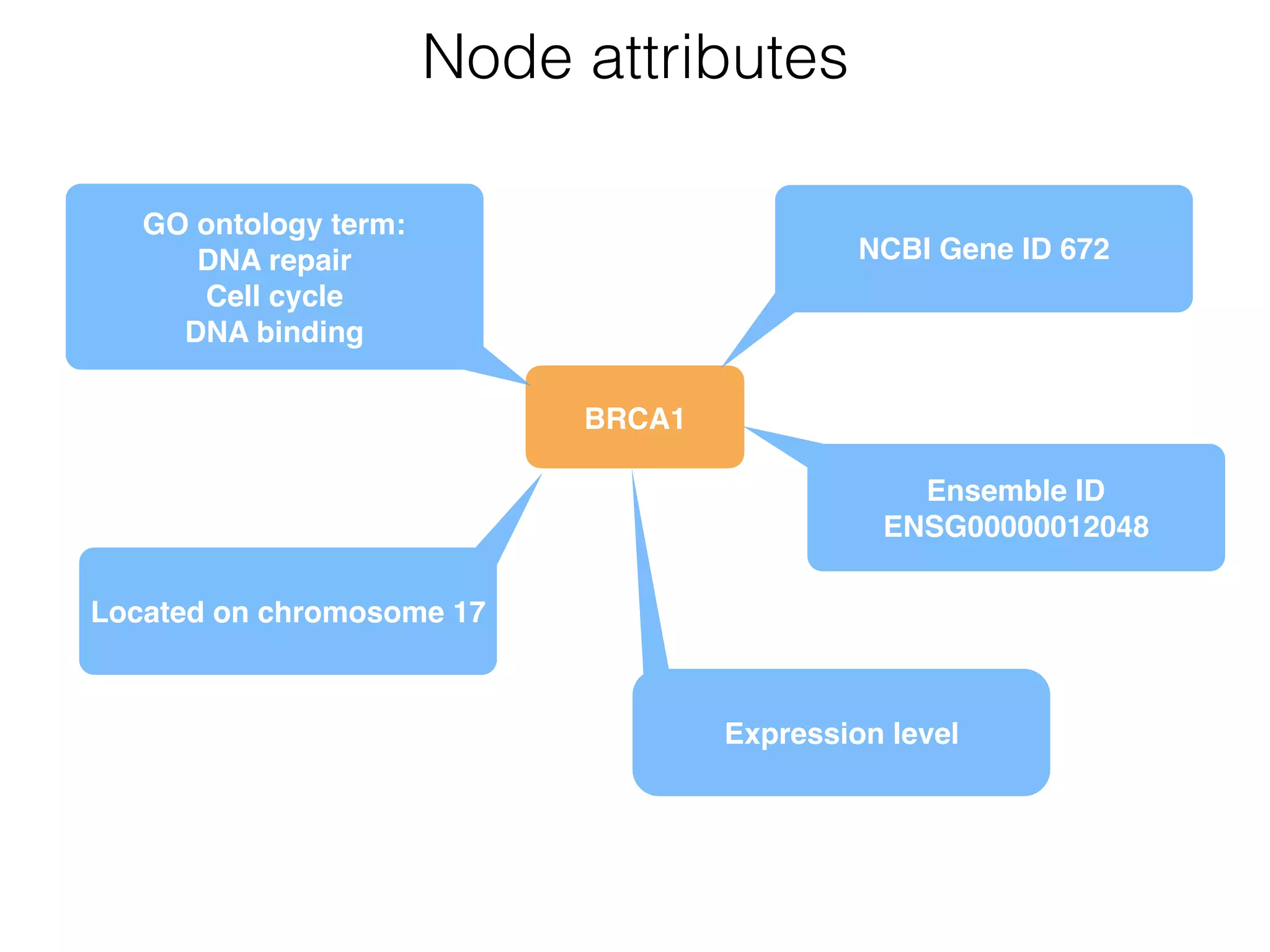
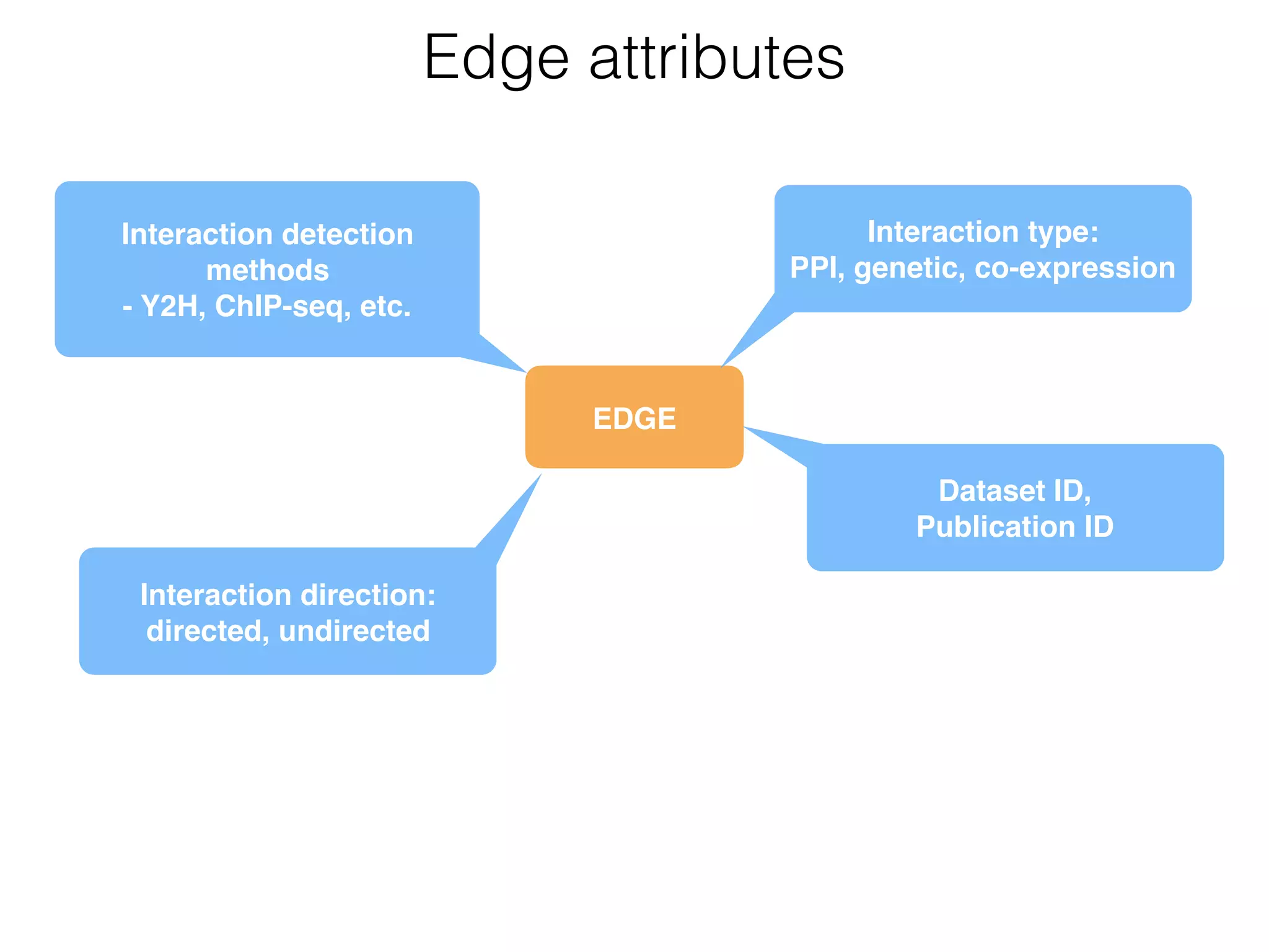
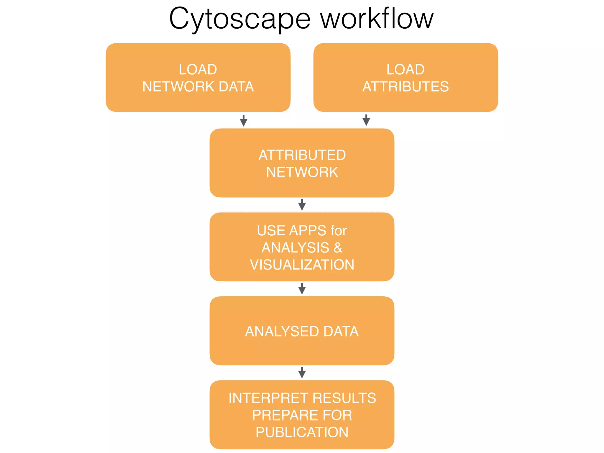
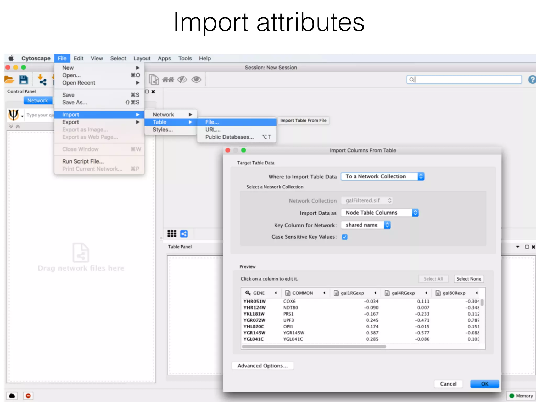
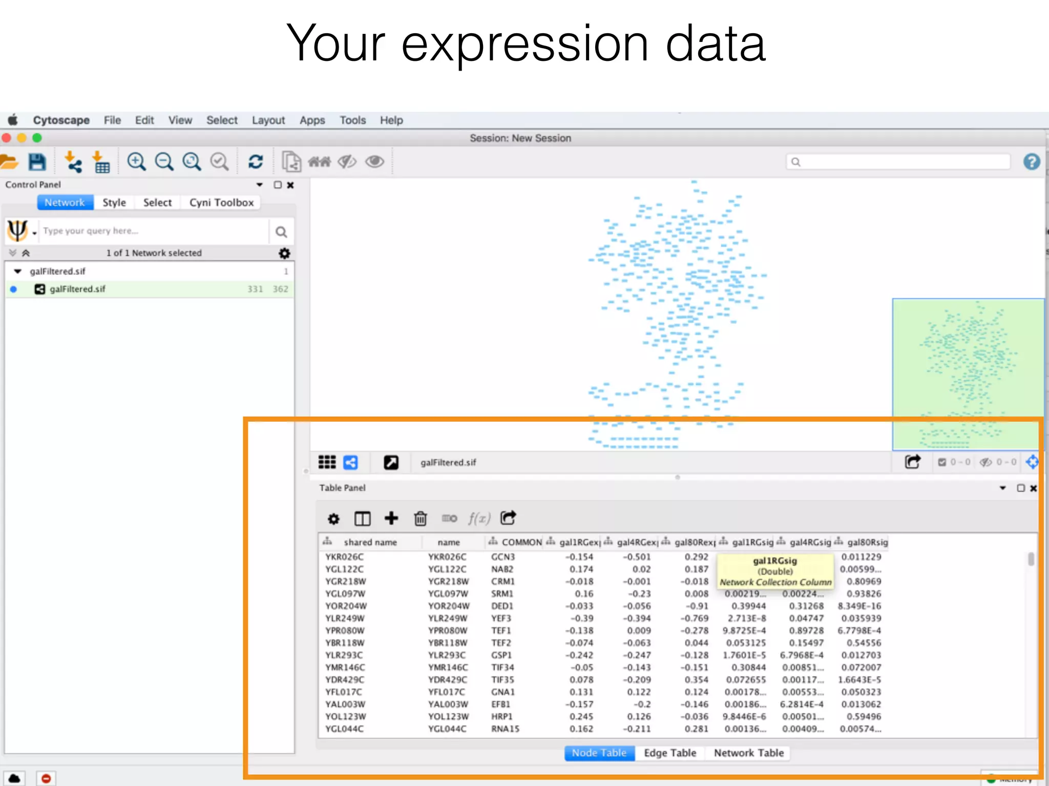
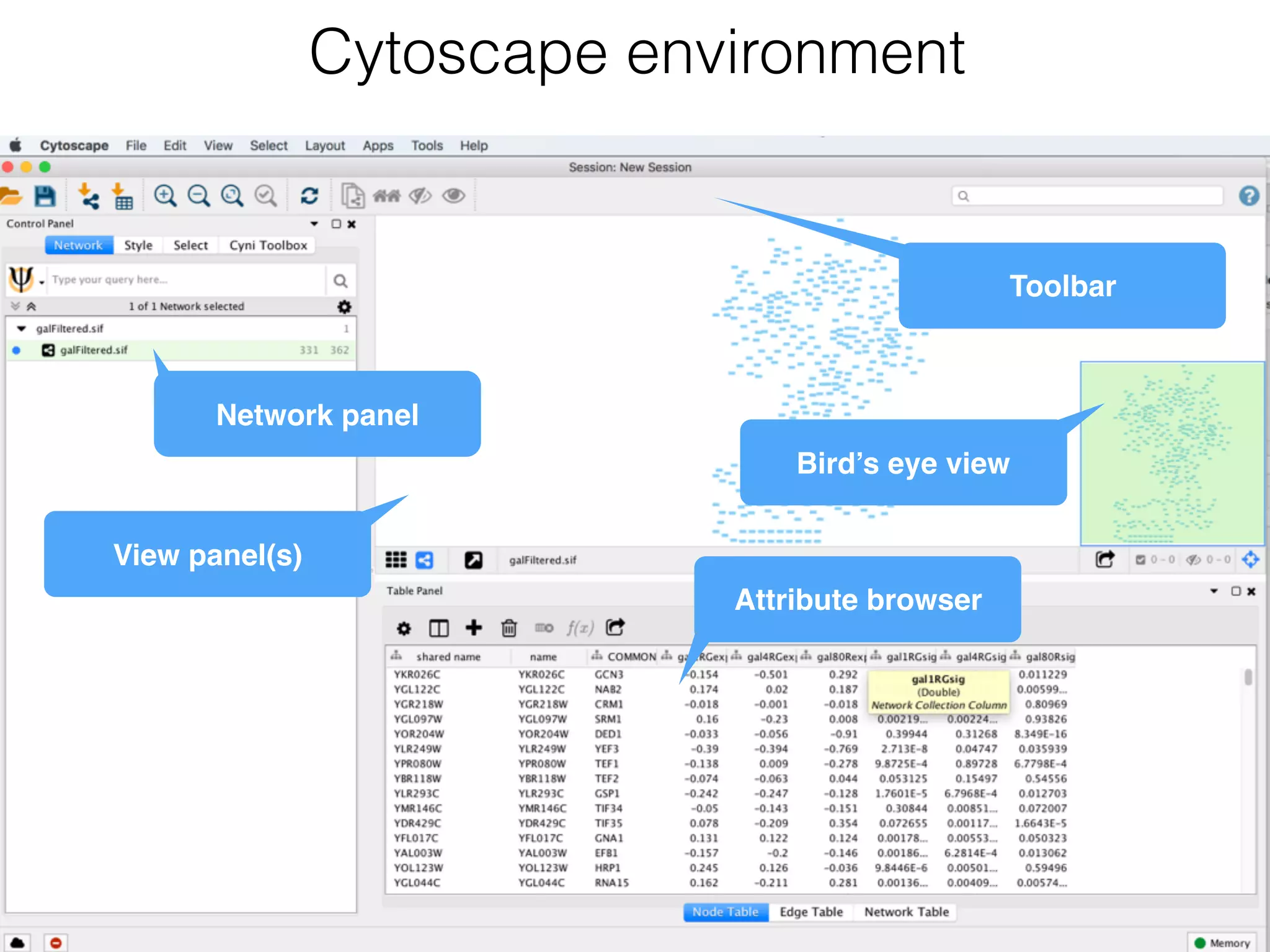
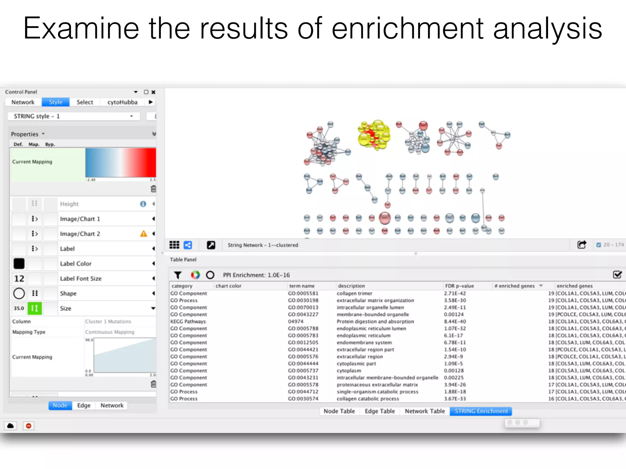
Interpretation of the biological knowledge
using networks approach

Practice Session IV
Elena Sügis
elena.sugis@.ut.ee
Bioinformatics for bioengineers LTTI.00.016, Spring 2018
Stickers
Everything is fine Some help won’t hurt
• Basic Concepts

• Browsing Network Data

• Networks and Attributes

• Visualization Techniques

• Basic Analysis

• Expression Data Analysis

• Advanced Topics
Agenda
Prerequisites
• Cytoscape ver. 3.6.0

• Apps: 

- clusterMaker2

- ClueGo

- stringApp

- Diffusion
Before the practice session
please install the following software:
http://www.cytoscape.org/index.html
• Download Cytoscape application
• Follow the installation instructions
- you might be asked to install Java 8
• Go to
Get Cytoscape
Install Apps
1
2
Open App manager
Type the app name &

hit install
https://goo.gl/keRXcj
Data download
galExpData.csv
galFiltered.sif
• Go to
• Download 2 files:
Cytoscape is a tool for visualising and extracting
meaningful information, or modules out of large biological
networks.
Cytoscape core concepts
Nodes = any object
• Genes
• Proteins
• Metabolites
• Enzymes
• Organisms
6
3
4
5
2
1
Edges = biological relationship
• Interactions
• Regulations
• Reactions
• Transformations
• Activations
• Inhibitions
etc.
Cytoscape core concepts
• Networks
• Attributes
Nodes = any object
• Genes
• Proteins
• Metabolites
• Enzymes
• Organisms
6
3
4
5
2
1
Edges = biological relationship
• Interactions
• Regulations
• Reactions
• Transformations
• Activations
• Inhibitions
etc.
Cytoscape core concepts
• Networks
• Attributes
Nodes = any object
• Genes
• Proteins
• Metabolites
• Enzymes
• Organisms
6
3
4
5
2
1
Edges = biological relationship
• Interactions
• Regulations
• Reactions
• Transformations
• Activations
• Inhibitions
etc.
Network representation:
1 - 2
1 - 5

2 - 3

2 - 5
3 - 4
4 - 5
4 - 6
Attributes = any data about
nodes,edges and networks
Cytoscape core concepts
• Networks
• Attributes
Nodes = any object
• Genes
• Proteins
• Metabolites
• Enzymes
• Organisms
6
3
4
5
2
1
Edges = biological relationship
• Interactions
• Regulations
• Reactions
• Transformations
• Activations
• Inhibitions
etc.
Network representation:
1 - 2
1 - 5

2 - 3

2 - 5
3 - 4
4 - 5
4 - 6
ID
alternative 

name
expression
1 Nanog 2.5
2 Oct4 2
3 Pax6 1.3
… … …
5 Sox2 3.2
ID co-expression
1-2 0.8
1-5 0.75
2-3 0.4
… …
4-6 0.65
node attributes edge attributes
Attributes = data tables
BRCA1
Node attributes
GO ontology term:

DNA repair

Cell cycle

DNA binding
BRCA1
Node attributes
NCBI Gene ID 672
Ensemble ID
ENSG00000012048
GO ontology term:

DNA repair

Cell cycle

DNA binding
BRCA1
Node attributes
NCBI Gene ID 672
Ensemble ID
ENSG00000012048
GO ontology term:

DNA repair

Cell cycle

DNA binding
Located on chromosome 17
BRCA1
Node attributes
NCBI Gene ID 672
Ensemble ID
ENSG00000012048
GO ontology term:

DNA repair

Cell cycle

DNA binding
Located on chromosome 17
Expression level
EDGE
Edge attributes
Interaction type:
PPI, genetic, co-expression
Dataset ID, 

Publication ID
Interaction detection
methods
- Y2H, ChIP-seq, etc.
Interaction direction:

directed, undirected
Cytoscape is a tool for:
• Visualisation
• Network data analysis
• Data integration (join networks and attributes, direct
access to remote data sources)
Cytoscape workflow
LOAD

NETWORK DATA
LOAD

ATTRIBUTES
ATTRIBUTED 

NETWORK
ANALYSED DATA
INTERPRET RESULTS

PREPARE FOR

PUBLICATION
USE APPS for

ANALYSIS &

VISUALIZATION
Network data formats
• SIF
• GML
• XGMML
• GraphML
• BioPAX
• PSI-MI
• SBML
• KGML (KEGG)
• Excel
• Delimited Text
• Table
• CSV
• Tab
• Any table data can be imported to Cytoscape by Table
Import function
• Preparing your table data with widely-used ID is important
for easy mapping
Cytoscape supports many standard network data formats
Load network 

data & attributes
Demo1
• Understand Basic UI.

• Load sample network and attributes files.

• Learn how to browse the network and attributes.
Goal
Your data


• 2 files:
network data galFiltered.sif
attributes data galExpData.csv
• Files describe yeast transcription factors (Gal1, Gal4, and
Gal80) experiments. 

Have a look at the network file


• Use text redactor of your choice and open file galFiltered.sif
• What do you see?

Network data
Node A ID
Node B ID
Interaction type
Import network
Import network to cytoscape


• Start Cytoscape and load the network via File → Import → Network
→ File.

• When the network first opens, the entire network might not be visible
because of the default zoom factor used. To see the whole network,
select View → Fit Content.

Imported network
Have a look at the attributes file


• Use text redactor of your choice and open file galExpData.csv
• What do you see?

Attribute data
Node ID

(here yeast locus tag)
Gene
common name
Node IDs must match the names of the nodes in your network exactly!
Gene expression 

in 3 conditions
Significance of change
in expression
Import attributes
Your expression data
Cytoscape environment
View panel(s)
Attribute browser
Toolbar
Bird’s eye view
Network panel
Data mapping to
visual styles
Demo 2
• Help scientists to understand their data sets.
• Tell a biological story.
Goal of scientific data visualization
Layouts
Circular Spring-embedded Hierarchical
Select layout
• Visual attributes
- Node fill colour, border colour, border width, size, shape,
opacity, label
-Edge type, colour, width, ending type, ending size,
ending colour

• Mapping types
- Continuous (numeric values)
- Discrete (categories)
- Passthrough (labels)
Data Mapping to visual styles
6
3
4
5
2
1
Map data values associated with graph elements onto graph visuals
Change labels
Zoomed in view
1
2
Mapping Expression Data to Networks
• Open the Styles interface by selecting its tab in the Control
Panel (the leftmost panel). We are going to use the "COMMON"
name attribute to give the nodes useful names:
• Zoom in on the network so that node labels are visible.
• Click the second column of the "Label" row in the Styles panel.
This should produce a drop-down panel with Column and
Mapping Type.
• Change the "Column" to COMMON by clicking on the field to
the right of the Column label. This should bring up a list of
columns. Select COMMON.
• Verify that the node labels on the network have changed to their
common names.
• By default, the Mapping Type is Passthrough Mapping, which
is what we want to use. Other options are Discrete Mapping and
Continuous Mapping.
Select expression column
Map gradient colour
Map expression to node colour
• Click on the middle square (Map.) next to the Fill Color row in the
Styles panel.
• Click the -- select value -- cell in the Column section.
• In the drop-down menu of available column names, select
"gal80Rexp".
• Click the -- select value-- cell in the Mapping Type section.
• In the drop-down menu of available mapping types, select Continuous
Mapping.
• This action will produce a gradient ranging from blue to red.
• Click on the color gradient to change the colors. This will pop-up a
gradient editing dialog.
• We're going to build a basic blue-white-yellow gradient for our
expression values.
Create your style
1
2
• Change the gradient in node fill colour.
• Drag the left-most, black inverted triangle handle along the top of
the gradient. Drag it to an value of approx -1.2. Double-click on the
handle and set a colour in the blue range.
• Drag the white inverted triangle handle to approx 0.5. You can type
the value in the Handle Position section to be more precise.
• Add a new handle by clicking Add, and drag that handle to 2.5. Set
the colour to yellow.
• Finally, set the Maximum Color by double-clicking on the white, left-
pointing triangle. Set it to green.
• You can also change the colour of each handle by double-clicking or
using the Node Fill Color selector button in the Handle Settings
section.
Create your own style
New gradient schema
• This should produce a Blue-White-Yellow Color gradient like the image
below, with min and max extremes coloured black and green,
respectively.
• Click OK to save the gradient adjustment dialog and verify that the
nodes in the network reflect the new colouring scheme.
Colour the default node
Set the node shape
• Use the significance values to change the shape of the nodes.

• So that high confidence measurements will appear as squares while
potentially bad measurements appear as circles.
1
2
3
Set the node shape
Network will look like
Exercise
• Use default visual mapping style.
• Set Default Node Color for nodes with no data mapping as dark
grey.
• Set nodes with expression values that are significant to be
rendered as rectangles, others are ovals.
• Set the common name for each gene as the Node Label.
• Apply circular layout.
Exercise
Resulting network view
Basic gene
expression analysis
demo 3
• Visualise networks using expression data.
• Filter networks based on expression data.
• Assess expression data in the context of a biological
network.
Goal
Network interaction types
1
Filter out pp interactions
32
Selected interactions are
highlighted red
Delete pp interactions
Since we're only interested in the protein-DNA edges, we can
delete the protein-protein edges we've just selected.

• To delete selected nodes or edges use the menu Edit → Delete
Selected Nodes and Edges.
• Clean up the network view by applying a force-directed layout
Layout → Prefuse Force Directed Layout.
Resulting network view
• Notice that three dark red (highly
induced) nodes are in the same
region of the graph.
• Notice that there are two nodes
that interact with all three red
nodes: GAL4 (YPL248C) and
GAL11 (YOL051W).
• Let's select these two nodes and
their first neighbours
Selecting first neighbours
1
2
Network from first neighbours
3
4
Interpreting the results
GAL4 is repressed by GAL80
GAL4 and GAL11 show fairly
small changes in expression, not
statistically significant
Interpreting the results
GAL4 is repressed by GAL80
GAL4 and GAL11 show fairly
small changes in expression, not
statistically significant
Significant level of repression
Interpreting the results
GAL4 is repressed by GAL80
GAL4 and GAL11 show fairly
small changes in expression, not
statistically significant
Significant level of repression
Most interactions of GAL4 are
significantly unregulated
• Transcriptional activation activity of Gal4 is repressed by Gal80.
• Repression of Gal80 increases the transcriptional activation
activity of Gal4. Expression of Gal4 itself did not change much,
but Gal4 transcripts were much more likely to be active
transcription factors when Gal80 was repressed.
• This explains why there is so much up-regulation in among
Gal4 interactors.
Summary
Get more info about the gene
• Right-click on the node GAL4.
• Select the menu External Links → Sequences and Proteins
→ Ensembl Gene View.
• This action will pop-up a browser window and search the
Ensembl database for the term "YPL248C", the id of the node.
• The description of GAL4 tells us that it is repressed by
GAL80.
1
2
Saving results
Cytoscape provides a number of ways to save results and visualizations:
• As a session: File→Save, File→Save As
• As an image: File→Export as Image
• To the web: File→Export as Web Page
• To a public repository: File → Export → Network Collection to NDEx
• As a graph format file: File → Export → Network.
Network formats:
• CX JSON
• Cytoscape.js JSON
• GraphML
• PSI-MI
• XGMML
• SIF
Saving the results
Save the session
Export as network,

table, image, etc
Interpretation of the biological knowledge
using networks approach

Practice Session V
Elena Sügis
elena.sugis@.ut.ee
Bioinformatics for bioengineers LTTI.00.016, Spring 2018
Stickers
Everything is fine Some help won’t hurt
• Exploratory analysis

• Computing network statistics

• Mapping statistics to visuals

• Expression clustering

• Combining your dataset with external data

• Community detection

• Functional enrichment analysis
Agenda
Prerequisites
• Cytoscape ver. 3.6.0

• Apps: 

- clusterMaker2

- ClueGo

- stringApp

- Diffusion
Before the practice session
please install the following software:
http://www.cytoscape.org/index.html
• Download Cytoscape application
• Follow the installation instructions
- you might be asked to install Java 8
• Go to
Get Cytoscape
Install Apps
1
2
Open App manager
Type the app name &

hit install
https://goo.gl/keRXcj
Data download
GBM-TP-all.tsv

GSE6887_Bcell_Healthy_top200UpRegulated.txt
GSE6887_NKcell_Healthy_top200DownRegulated.txt
GSE6887_NKcell_Healthy_top200UpRegulated.txt
• Go to
• Download files:
galFiltered.sif
galExpData.csv
• Download 2 files (if you haven’t attend practice session IV):
Or ask a friend to share existing Cytoscape session .cys file
Network statistics
demo 4
• Calculate network statistics by Network Analyzer
• Filter network based on statistics

• Map statistics to visual style

Goal
Provides basic statistics
of networks:
• Degree
• Centrality
• Shortest Path Length Distribution
• etc
Network Analyzer
Let’s refresh our
knowledge from the
lecture
Degree distribution
Degree of a node is the number of edges incident to the node.…
Degree distribution
Degree of a node is the number of edges incident to the node.
Degree distribution in a biological network
• Networks with power-law degree distributions are called scale-free
networks
• Most nodes are of low degree, but there is a small number of
highly-linked nodes (nodes of high degree) called “hubs.”
P(k) ~ k−γ
Image is adapted from E. Ravasz et al., Science, 2002
Shortest path
• Distance between two nodes is the smallest number of links that
have to be traversed to get from one node to the other.

Shortest path is the path that achieves that distance.

• Small world network is characterised by small average path length
l =
2
N(N −1)
lij
i<j
∑
lij is the shortest path length between node i and j
Figure is partially adapted with modifications from original https://cytoscape.github.io/cytoscape-tutorials/presentations/modules/network-analysis/index.html#/0/6
How different centralities look
HUB
node that connect two sub-networks
closest node to all other nodes
Biological meaning
Degree centrality Closeness centralityBetweenness centrality
• Amount of control that
this node has over the
interactions of other
nodes in the network

• How much information
load is on the node

• Describes connectivity of
the network

• Nodes that connect two
sub-networks

• Can be calculated for
edges as well
• Nodes with a high
degree are also called
hub nodes

• Real networks have many
nodes with low degree
and few nodes with high
degree

• Nodes with a high
degree tend to be
essential nodes

• Regulatory elements like
transcription factors often
have a high out-degree
• Indication for how fast
information spreads from
a given node to other
reachable nodes in the
network
• The more central a node
is, the smaller is the
distance to all other
nodes, the higher is the
closeness
Material is adapted from BioSB 2015 Network Analysis Course
• Open the session that you have saved File → Open 

Open saved session
OR if you haven’t saved the session
Create network from scratch:

• Start Cytoscape and load the network via File → Import →
Network → File (galFiltered.sif).

• When the network first opens, the entire network might not be
visible because of the default zoom factor used. To see the whole
network, select View → Fit Content.

• Import attributes File → Import → Table → File (galExpData.csv)

Import attributes
Compute summary network statistics
Inspect the results
• Inspect the results
• Does degree distribution follows power law?
Inspect the results
• Inspect the results
• Does degree distribution follows power law?
Network statistics as attributes
Arrange attribute columns showing node
Degree

Betweenness centrality

Clustering coefficient
• NetworkAnalyzer provides all results as regular attributes
• Can be used for filtering
• What are 3 top nodes with the highest betweenness centrality?

• What are 3 top nodes with the highest degree?
• What nodes have the highest clustering coefficient?
Observe your results
Map network statistics to visual style
Use node degree to change the size of the nodes
Filtering based on network statistics
• Select nodes with degree ≥ 5 and their first neighbours
• Create a new subnetwork from the selection
Filtering based on network statistics
• Select nodes with degree ≥ 5 and their first neighbours
• Create a new subnetwork from the selection
Sub-network from connected components
Sub-network from the largest
connected component
Functional enrichment
workflow
demo 5
• Retrieve networks and pathways

• Integrate and explore your data

• Perform functional enrichment analysis

• Functional interpretation
Goal
Get the data
• Download GBM-TP.all.tsv from https://goo.gl/keRXcj
• Open the file in your favourite text editor. Observe file content. Can we
create a network from this file?
• Import the file to create a network using File → Import → Network →
File.
• This will bring up the Import Network From Table dialog.
• Select Select None to disable all columns.
• Click only on the GeneName column and set this column as the
Source Node column (green circle).
• Click OK. You’ll see a warning about no edges, but that’s OK. This will
create a grid of 1500 unconnected nodes, where each node
represents a gene.
Add attributes
• Open the file again, but now use File → Import → Table → File. 

• This will bring up the Import Columns From Table dialog.
It turns out that all of the defaults are correct for just importing the
data, so click on OK.
This will import all of the data in the spreadsheet and associate
each row with the corresponding node.

• You should be able to see this in the Table Panel.
• Open the Select tab and click on the + button
to add a new condition. In this case we’re going
to add a Column Filter. 

• Select the "Mean log2FC" column and set the
values to be between -5 and -1. This will select
all genes that are significantly underexpressed
on average, across all samples (only one gene
should be selected).

• Repeat the same process as above, but set the
values to be between 1 and 5. You’ll also need
to change the type of match (at the top of the
panel) to Match any (OR). No additional genes
will be selected in this case (but this approach
will be reused later).
Find significant expression changes
Genes with significant average expression
changes across all samples
How many genes have you detected?
Genes with significant average expression
changes across all samples
RPS4Y1
protein that is linked to
glioblastoma
Only one gene…
• It is a relatively unsatisfying result that only a single protein changes
expression in glioblastoma patients. 

• Let’s have a closer look at our data.
• Cluster all of the data.

• Find significant patterns in the data.

• Apply clusterMaker2 is a Cytoscape app that provides a number of
clustering algorithms including hierarchical and k-means.
Find significant expression changes
• Perform hierarchical clustering.

• In Cytoscape, select Apps → clusterMaker → Hierarchical cluster. 

This will bring the settings for hierarchical clustering. Select select all of
the samples (TCGA-*) in Node Attributes for cluster list. 

• The checkboxes Cluster attributes as well as nodes, Ignore nodes/
edges with no data, and Show TreeView when complete should all be
checked. Then click OK. The resulting TreeView should look like the figure
on the next slide.
Find significant expression changes
• Looking at the result, is seems like there are definite bands of expression data that
look similar across a group of patients, but differ between groups. 

• Let’s take that known data and see if we can subset the data into 4 subtypes.
Hierarchical clustering result
• Select Apps → clusterMaker → K-Means cluster.
• In the resulting settings dialog, set the number of cluster to 4, which
is the number of known subtypes of glioblastoma, as with the
hierarchical cluster.

• Select all of the samples (TCGA-*), check Cluster attributes as
well as nodes and Show HeatMap when complete. 

• This will result in a heat map similar to the one in the figure on the next
slide.
K-means clustering
K-means clustering result
Find significant expression
changes in Cluster 1
• Open the Select tab.
• Use Column Filters for the "Cluster 1 Mean log2FC" column.

Select the "Cluster 1 Mean log2FC" column and set the values to be
between -5 and -1, then add a second filter (be sure to specify OR at
the top) and set the values between 1 and 5.

• This should result in a selection of 171 nodes.
Download the PPI from STRING
• Select gene names from Table Panel.
• Paste gene names into STRING network search. 

• In the Network tab of the Control Panel at the top should be a
text field with an icon at the left.
• Select STRING protein query. (If you don’t see any STRING
options, the stringApp hasn’t been loaded.) Then click into the text
field and paste the list of genes.

• Set STRING search parameters. Next to the text field is a menu
with a list of options. Change the Confidence (score) cutoff to 0.8
and the Maximum additional interactors to 30. This will get only
high quality results (80% confidence) and add 30 extra proteins to
the network.
Load the network
Style the network to show differential
expression
• Re-import expression data. Similar to the initial import, start by doing File
→ Import → Table → File. Again, select the GBM-TP-all.tsv file.
• Change the Key Column for Network: from share name to query term.
• STRING uses Ensembl identifiers, but retains the original query term so
we can match data against. Now select OK.
• Disable structure image. Disable the images by going to Apps →
STRING → Don’t show structure images.
• Create colour gradient for expression data.
Add styling to show mutations
• Lock node width and height. By default, the stringApp provides
separate values for Node Width and Node Height. In our case, we
just want to lock them to be the same so we only have to modify the
Node Size. The Lock node width and height is a checkbox at the
bottom of the Node tab in the Style tab of the Control Panel. Make
sure that it’s checked.
• Set the default node size. Click on the leftmost (Def.) box next to
Size. Set the default size to "45.0".
Map mutation to node size
Choose "Cluster 1 Mutations" for the Column and "Continuous Mapping" for the
Mapping Type
Examine the network
overexpressed genes,

exhibit some mutations
underexpressed genes,

exhibit some mutations
Community detection
demo 6
Community detection
Figure is adapted from original https://cytoscape.github.io/cytoscape-tutorials/presentations/advanced-automation-2017-mpi.html#/11
Identifying closely-related groups of nodes (modules/clusters)
• Based on topology
• Based on a shared function(s)
Cluster network using MCL
• Go to Apps → clusterMaker → MCL Cluster
• Create new clustered network
Functional enrichment
Your gene

list
• Each module contains a list of genes.

• You want to know ….
Functional enrichment
Does your gene list includes more
genes with function x than expected by
random chance?
Genes with
known

function x
?
Your gene

list
Set network as a STRING network
• Set network as a STRING network. A menu item is available for that
purpose: Apps → STRING → Set as STRING network.
• Retrieve functional enrichment of a component. through the

Apps → STRING → Retrieve functional enrichment.
• What are the top 3 biological processes that you observe?

• Where do biological processes take place?

• How many genes are enriched?

• Find top 3 biological pathways?
Study the results
Examine the results of enrichment analysis
Advanced enrichment
analysis and visualisation
using ClueGO
demo 7
• From Gene Expression Omnibus GSE6887, a gene expression
profile of peripheral blood lymphocytes of melanoma patients and
healthy controls.
• We will use expression profiles of B cells and NK cells in healthy
controls.
• We calculated a mean of the existing replicates for each immune
cells of interests. The genes were sorted based on their expression
for each, B and NK cells respectively.
• The top 200 most expressed genes were included in the list with up
regulated genes and the top 200 lowest expressed genes in the list
with down regulated genes.
• The reference used in this dataset was a pool of all immune cell
types.
• We lists with the top 200 up regulated genes and the top 200 down
regulated genes for B cells and NK cells.
Data
ClueGO options
gene list of interest goes here
Select ontologies, i.e. GO,
KEGG, Reactome
Choose evidence, i.e
experimental, inferred from
source A/B/C
Choose type of hypergeometric
test and correction method
• Open application Apps → ClueGO
Analysis of gene list
• Open file GSE6887_Bcell_Healthy_top200UpRegulated.txt

• Copy gene IDs.
• Paste gene IDs to “Load Marker list(s)”.

• Select KEGG and Reactome pathways in the ontology settings.

• Select “All” in evidence settings.
• Retrieve functional enrichment of a component.
ClueGO settings
1
2
3
gene list of interest goes here
Select KEGG and
Reactome
Select all evidence
Resulting view pathway enrichment analysis
ClueGO result
Leading term (has the highest
significance the group)
Term name Term p-value Associated genes

information (% of all
genes in the term,
number of genes,

gene names)
Histogram with terms
Term name Term significance
Associated genes

information (% of found genes
compared to all the genes associated
with the term)
Associated genes

information (# of the genes from the
analysed gene list found
associated with the term)
** term/group p-value<0.001
* term/group 0.001<p-value<0.05
. (dot) 0.05<p-value<0.01
Overview chart with functional groups
The name of the group is given by the group leading term (e.g. the most significant term in the group).
Show genes together with terms
Add/remove genes

related to pathways
Gene is associated
with 2 pathways
Visualise terms associated with the gene
Add/remove terms
from the network
Gene is associated
with 2 pathways
Add interactions from external source
1
2
3
Gene/Interaction Enrichment Options
Physical interactions
in your enriched
group of genes
Add interactions from external source
1
2
3
Gene/Interaction Enrichment Options
Physical interactions
in your enriched
group of genes
NOTE: you can define gene modules based on genes related to
term/group of terms additionally/instead of topology-based rules
Enrichment comparison
in 2 groups using
ClueGO
demo 8
Data
Use the gene lists from the files related to up/down regulated genes in
natural killer cells in healthy controls:
• GSE6887_NKcell_Healthy_top200DownRegulated.txt
• GSE6887_NKcell_Healthy_top200UpRegulated.txt
Select module for the analysis
Open file
GSE6887_NKcell_Healthy_top
200UpRegulated.txt
Open file
GSE6887_NKcell_Healthy_top
200DownRegulated.txt
Select ontologies,

use KEGG, Reactome
Change node shape for

KEGG and Reactome
Explore the network
Observe over represented terms in each cluster or in the overall group.
Explore the network
Find terms related to two or more groups
Explore the network
Find terms related to two or more groups
Colour the network based on clusters
Explore enriched processed
• Find interesting genes/groupings
• Find the 3 top significant pathways enriched with Down-reagulated genes
• Find the 3 top significant pathways enriched with Up-reagulated genes

Practice discovering biological knowledge using networks approach.

  • 1.
    Interpretation of thebiological knowledge using networks approach
 Practice Session IV Elena Sügis elena.sugis@.ut.ee Bioinformatics for bioengineers LTTI.00.016, Spring 2018
  • 2.
    Stickers Everything is fineSome help won’t hurt
  • 3.
    • Basic Concepts
 •Browsing Network Data
 • Networks and Attributes
 • Visualization Techniques
 • Basic Analysis
 • Expression Data Analysis
 • Advanced Topics Agenda
  • 4.
    Prerequisites • Cytoscape ver.3.6.0
 • Apps: 
 - clusterMaker2
 - ClueGo
 - stringApp
 - Diffusion Before the practice session please install the following software:
  • 5.
    http://www.cytoscape.org/index.html • Download Cytoscapeapplication • Follow the installation instructions - you might be asked to install Java 8 • Go to Get Cytoscape
  • 6.
    Install Apps 1 2 Open Appmanager Type the app name &
 hit install
  • 7.
  • 8.
    Cytoscape is atool for visualising and extracting meaningful information, or modules out of large biological networks.
  • 9.
    Cytoscape core concepts Nodes= any object • Genes • Proteins • Metabolites • Enzymes • Organisms 6 3 4 5 2 1 Edges = biological relationship • Interactions • Regulations • Reactions • Transformations • Activations • Inhibitions etc.
  • 10.
    Cytoscape core concepts •Networks • Attributes Nodes = any object • Genes • Proteins • Metabolites • Enzymes • Organisms 6 3 4 5 2 1 Edges = biological relationship • Interactions • Regulations • Reactions • Transformations • Activations • Inhibitions etc.
  • 11.
    Cytoscape core concepts •Networks • Attributes Nodes = any object • Genes • Proteins • Metabolites • Enzymes • Organisms 6 3 4 5 2 1 Edges = biological relationship • Interactions • Regulations • Reactions • Transformations • Activations • Inhibitions etc. Network representation: 1 - 2 1 - 5
 2 - 3
 2 - 5 3 - 4 4 - 5 4 - 6
  • 12.
    Cytoscape core concepts •Networks • Attributes Nodes = any object • Genes • Proteins • Metabolites • Enzymes • Organisms 6 3 4 5 2 1 Edges = biological relationship • Interactions • Regulations • Reactions • Transformations • Activations • Inhibitions etc. Network representation: 1 - 2 1 - 5
 2 - 3
 2 - 5 3 - 4 4 - 5 4 - 6 Attributes = any data about nodes,edges and networks
  • 13.
    Cytoscape core concepts •Networks • Attributes Nodes = any object • Genes • Proteins • Metabolites • Enzymes • Organisms 6 3 4 5 2 1 Edges = biological relationship • Interactions • Regulations • Reactions • Transformations • Activations • Inhibitions etc. Network representation: 1 - 2 1 - 5
 2 - 3
 2 - 5 3 - 4 4 - 5 4 - 6 ID alternative 
 name expression 1 Nanog 2.5 2 Oct4 2 3 Pax6 1.3 … … … 5 Sox2 3.2 ID co-expression 1-2 0.8 1-5 0.75 2-3 0.4 … … 4-6 0.65 node attributes edge attributes Attributes = data tables
  • 14.
    BRCA1 Node attributes GO ontologyterm:
 DNA repair
 Cell cycle
 DNA binding
  • 15.
    BRCA1 Node attributes NCBI GeneID 672 Ensemble ID ENSG00000012048 GO ontology term:
 DNA repair
 Cell cycle
 DNA binding
  • 16.
    BRCA1 Node attributes NCBI GeneID 672 Ensemble ID ENSG00000012048 GO ontology term:
 DNA repair
 Cell cycle
 DNA binding Located on chromosome 17
  • 17.
    BRCA1 Node attributes NCBI GeneID 672 Ensemble ID ENSG00000012048 GO ontology term:
 DNA repair
 Cell cycle
 DNA binding Located on chromosome 17 Expression level
  • 18.
    EDGE Edge attributes Interaction type: PPI,genetic, co-expression Dataset ID, 
 Publication ID Interaction detection methods - Y2H, ChIP-seq, etc. Interaction direction:
 directed, undirected
  • 19.
    Cytoscape is atool for: • Visualisation • Network data analysis • Data integration (join networks and attributes, direct access to remote data sources)
  • 20.
    Cytoscape workflow LOAD
 NETWORK DATA LOAD
 ATTRIBUTES ATTRIBUTED
 NETWORK ANALYSED DATA INTERPRET RESULTS
 PREPARE FOR
 PUBLICATION USE APPS for
 ANALYSIS &
 VISUALIZATION
  • 21.
    Network data formats •SIF • GML • XGMML • GraphML • BioPAX • PSI-MI • SBML • KGML (KEGG) • Excel • Delimited Text • Table • CSV • Tab • Any table data can be imported to Cytoscape by Table Import function • Preparing your table data with widely-used ID is important for easy mapping Cytoscape supports many standard network data formats
  • 22.
    Load network 
 data& attributes Demo1
  • 23.
    • Understand BasicUI.
 • Load sample network and attributes files.
 • Learn how to browse the network and attributes. Goal
  • 24.
    Your data 
 • 2files: network data galFiltered.sif attributes data galExpData.csv • Files describe yeast transcription factors (Gal1, Gal4, and Gal80) experiments. 

  • 25.
    Have a lookat the network file 
 • Use text redactor of your choice and open file galFiltered.sif • What do you see?

  • 26.
    Network data Node AID Node B ID Interaction type
  • 27.
  • 28.
    Import network tocytoscape 
 • Start Cytoscape and load the network via File → Import → Network → File.
 • When the network first opens, the entire network might not be visible because of the default zoom factor used. To see the whole network, select View → Fit Content.

  • 29.
  • 30.
    Have a lookat the attributes file 
 • Use text redactor of your choice and open file galExpData.csv • What do you see?

  • 31.
    Attribute data Node ID
 (hereyeast locus tag) Gene common name Node IDs must match the names of the nodes in your network exactly! Gene expression 
 in 3 conditions Significance of change in expression
  • 32.
  • 33.
  • 34.
    Cytoscape environment View panel(s) Attributebrowser Toolbar Bird’s eye view Network panel
  • 35.
  • 36.
    • Help scientiststo understand their data sets. • Tell a biological story. Goal of scientific data visualization
  • 37.
  • 38.
  • 39.
    • Visual attributes -Node fill colour, border colour, border width, size, shape, opacity, label -Edge type, colour, width, ending type, ending size, ending colour
 • Mapping types - Continuous (numeric values) - Discrete (categories) - Passthrough (labels) Data Mapping to visual styles 6 3 4 5 2 1 Map data values associated with graph elements onto graph visuals
  • 40.
  • 41.
    Mapping Expression Datato Networks • Open the Styles interface by selecting its tab in the Control Panel (the leftmost panel). We are going to use the "COMMON" name attribute to give the nodes useful names: • Zoom in on the network so that node labels are visible. • Click the second column of the "Label" row in the Styles panel. This should produce a drop-down panel with Column and Mapping Type. • Change the "Column" to COMMON by clicking on the field to the right of the Column label. This should bring up a list of columns. Select COMMON. • Verify that the node labels on the network have changed to their common names. • By default, the Mapping Type is Passthrough Mapping, which is what we want to use. Other options are Discrete Mapping and Continuous Mapping.
  • 42.
  • 43.
  • 44.
    Map expression tonode colour • Click on the middle square (Map.) next to the Fill Color row in the Styles panel. • Click the -- select value -- cell in the Column section. • In the drop-down menu of available column names, select "gal80Rexp". • Click the -- select value-- cell in the Mapping Type section. • In the drop-down menu of available mapping types, select Continuous Mapping. • This action will produce a gradient ranging from blue to red. • Click on the color gradient to change the colors. This will pop-up a gradient editing dialog. • We're going to build a basic blue-white-yellow gradient for our expression values.
  • 45.
  • 46.
    • Change thegradient in node fill colour. • Drag the left-most, black inverted triangle handle along the top of the gradient. Drag it to an value of approx -1.2. Double-click on the handle and set a colour in the blue range. • Drag the white inverted triangle handle to approx 0.5. You can type the value in the Handle Position section to be more precise. • Add a new handle by clicking Add, and drag that handle to 2.5. Set the colour to yellow. • Finally, set the Maximum Color by double-clicking on the white, left- pointing triangle. Set it to green. • You can also change the colour of each handle by double-clicking or using the Node Fill Color selector button in the Handle Settings section. Create your own style
  • 47.
    New gradient schema •This should produce a Blue-White-Yellow Color gradient like the image below, with min and max extremes coloured black and green, respectively. • Click OK to save the gradient adjustment dialog and verify that the nodes in the network reflect the new colouring scheme.
  • 48.
  • 49.
    Set the nodeshape • Use the significance values to change the shape of the nodes.
 • So that high confidence measurements will appear as squares while potentially bad measurements appear as circles.
  • 50.
  • 51.
  • 52.
  • 54.
    • Use defaultvisual mapping style. • Set Default Node Color for nodes with no data mapping as dark grey. • Set nodes with expression values that are significant to be rendered as rectangles, others are ovals. • Set the common name for each gene as the Node Label. • Apply circular layout. Exercise
  • 55.
  • 56.
  • 57.
    • Visualise networksusing expression data. • Filter networks based on expression data. • Assess expression data in the context of a biological network. Goal
  • 58.
  • 59.
    1 Filter out ppinteractions 32 Selected interactions are highlighted red
  • 60.
    Delete pp interactions Sincewe're only interested in the protein-DNA edges, we can delete the protein-protein edges we've just selected.
 • To delete selected nodes or edges use the menu Edit → Delete Selected Nodes and Edges. • Clean up the network view by applying a force-directed layout Layout → Prefuse Force Directed Layout.
  • 61.
    Resulting network view •Notice that three dark red (highly induced) nodes are in the same region of the graph. • Notice that there are two nodes that interact with all three red nodes: GAL4 (YPL248C) and GAL11 (YOL051W). • Let's select these two nodes and their first neighbours
  • 62.
  • 63.
    Network from firstneighbours 3 4
  • 64.
    Interpreting the results GAL4is repressed by GAL80 GAL4 and GAL11 show fairly small changes in expression, not statistically significant
  • 65.
    Interpreting the results GAL4is repressed by GAL80 GAL4 and GAL11 show fairly small changes in expression, not statistically significant Significant level of repression
  • 66.
    Interpreting the results GAL4is repressed by GAL80 GAL4 and GAL11 show fairly small changes in expression, not statistically significant Significant level of repression Most interactions of GAL4 are significantly unregulated
  • 67.
    • Transcriptional activationactivity of Gal4 is repressed by Gal80. • Repression of Gal80 increases the transcriptional activation activity of Gal4. Expression of Gal4 itself did not change much, but Gal4 transcripts were much more likely to be active transcription factors when Gal80 was repressed. • This explains why there is so much up-regulation in among Gal4 interactors. Summary
  • 68.
    Get more infoabout the gene • Right-click on the node GAL4. • Select the menu External Links → Sequences and Proteins → Ensembl Gene View. • This action will pop-up a browser window and search the Ensembl database for the term "YPL248C", the id of the node. • The description of GAL4 tells us that it is repressed by GAL80. 1 2
  • 69.
    Saving results Cytoscape providesa number of ways to save results and visualizations: • As a session: File→Save, File→Save As • As an image: File→Export as Image • To the web: File→Export as Web Page • To a public repository: File → Export → Network Collection to NDEx • As a graph format file: File → Export → Network. Network formats: • CX JSON • Cytoscape.js JSON • GraphML • PSI-MI • XGMML • SIF
  • 70.
    Saving the results Savethe session Export as network,
 table, image, etc
  • 71.
    Interpretation of thebiological knowledge using networks approach
 Practice Session V Elena Sügis elena.sugis@.ut.ee Bioinformatics for bioengineers LTTI.00.016, Spring 2018
  • 72.
    Stickers Everything is fineSome help won’t hurt
  • 73.
    • Exploratory analysis
 •Computing network statistics
 • Mapping statistics to visuals
 • Expression clustering
 • Combining your dataset with external data
 • Community detection
 • Functional enrichment analysis Agenda
  • 74.
    Prerequisites • Cytoscape ver.3.6.0
 • Apps: 
 - clusterMaker2
 - ClueGo
 - stringApp
 - Diffusion Before the practice session please install the following software:
  • 75.
    http://www.cytoscape.org/index.html • Download Cytoscapeapplication • Follow the installation instructions - you might be asked to install Java 8 • Go to Get Cytoscape
  • 76.
    Install Apps 1 2 Open Appmanager Type the app name &
 hit install
  • 77.
    https://goo.gl/keRXcj Data download GBM-TP-all.tsv
 GSE6887_Bcell_Healthy_top200UpRegulated.txt GSE6887_NKcell_Healthy_top200DownRegulated.txt GSE6887_NKcell_Healthy_top200UpRegulated.txt • Goto • Download files: galFiltered.sif galExpData.csv • Download 2 files (if you haven’t attend practice session IV): Or ask a friend to share existing Cytoscape session .cys file
  • 78.
  • 79.
    • Calculate networkstatistics by Network Analyzer • Filter network based on statistics
 • Map statistics to visual style
 Goal
  • 80.
    Provides basic statistics ofnetworks: • Degree • Centrality • Shortest Path Length Distribution • etc Network Analyzer
  • 81.
  • 82.
    Degree distribution Degree ofa node is the number of edges incident to the node.…
  • 83.
    Degree distribution Degree ofa node is the number of edges incident to the node.
  • 84.
    Degree distribution ina biological network • Networks with power-law degree distributions are called scale-free networks • Most nodes are of low degree, but there is a small number of highly-linked nodes (nodes of high degree) called “hubs.” P(k) ~ k−γ Image is adapted from E. Ravasz et al., Science, 2002
  • 85.
    Shortest path • Distancebetween two nodes is the smallest number of links that have to be traversed to get from one node to the other.
 Shortest path is the path that achieves that distance.
 • Small world network is characterised by small average path length l = 2 N(N −1) lij i<j ∑ lij is the shortest path length between node i and j
  • 86.
    Figure is partiallyadapted with modifications from original https://cytoscape.github.io/cytoscape-tutorials/presentations/modules/network-analysis/index.html#/0/6 How different centralities look HUB node that connect two sub-networks closest node to all other nodes
  • 87.
    Biological meaning Degree centralityCloseness centralityBetweenness centrality • Amount of control that this node has over the interactions of other nodes in the network
 • How much information load is on the node
 • Describes connectivity of the network
 • Nodes that connect two sub-networks
 • Can be calculated for edges as well • Nodes with a high degree are also called hub nodes
 • Real networks have many nodes with low degree and few nodes with high degree
 • Nodes with a high degree tend to be essential nodes
 • Regulatory elements like transcription factors often have a high out-degree • Indication for how fast information spreads from a given node to other reachable nodes in the network • The more central a node is, the smaller is the distance to all other nodes, the higher is the closeness Material is adapted from BioSB 2015 Network Analysis Course
  • 88.
    • Open thesession that you have saved File → Open 
 Open saved session OR if you haven’t saved the session Create network from scratch:
 • Start Cytoscape and load the network via File → Import → Network → File (galFiltered.sif).
 • When the network first opens, the entire network might not be visible because of the default zoom factor used. To see the whole network, select View → Fit Content.
 • Import attributes File → Import → Table → File (galExpData.csv)

  • 89.
  • 90.
  • 91.
    Inspect the results •Inspect the results • Does degree distribution follows power law?
  • 92.
    Inspect the results •Inspect the results • Does degree distribution follows power law?
  • 93.
    Network statistics asattributes Arrange attribute columns showing node Degree
 Betweenness centrality
 Clustering coefficient • NetworkAnalyzer provides all results as regular attributes • Can be used for filtering
  • 94.
    • What are3 top nodes with the highest betweenness centrality?
 • What are 3 top nodes with the highest degree? • What nodes have the highest clustering coefficient? Observe your results
  • 95.
    Map network statisticsto visual style Use node degree to change the size of the nodes
  • 96.
    Filtering based onnetwork statistics • Select nodes with degree ≥ 5 and their first neighbours • Create a new subnetwork from the selection
  • 97.
    Filtering based onnetwork statistics • Select nodes with degree ≥ 5 and their first neighbours • Create a new subnetwork from the selection
  • 98.
    Sub-network from connectedcomponents Sub-network from the largest connected component
  • 99.
  • 100.
    • Retrieve networksand pathways
 • Integrate and explore your data
 • Perform functional enrichment analysis
 • Functional interpretation Goal
  • 101.
    Get the data •Download GBM-TP.all.tsv from https://goo.gl/keRXcj • Open the file in your favourite text editor. Observe file content. Can we create a network from this file? • Import the file to create a network using File → Import → Network → File. • This will bring up the Import Network From Table dialog. • Select Select None to disable all columns. • Click only on the GeneName column and set this column as the Source Node column (green circle). • Click OK. You’ll see a warning about no edges, but that’s OK. This will create a grid of 1500 unconnected nodes, where each node represents a gene.
  • 102.
    Add attributes • Openthe file again, but now use File → Import → Table → File. 
 • This will bring up the Import Columns From Table dialog. It turns out that all of the defaults are correct for just importing the data, so click on OK. This will import all of the data in the spreadsheet and associate each row with the corresponding node.
 • You should be able to see this in the Table Panel.
  • 103.
    • Open theSelect tab and click on the + button to add a new condition. In this case we’re going to add a Column Filter. 
 • Select the "Mean log2FC" column and set the values to be between -5 and -1. This will select all genes that are significantly underexpressed on average, across all samples (only one gene should be selected).
 • Repeat the same process as above, but set the values to be between 1 and 5. You’ll also need to change the type of match (at the top of the panel) to Match any (OR). No additional genes will be selected in this case (but this approach will be reused later). Find significant expression changes
  • 104.
    Genes with significantaverage expression changes across all samples How many genes have you detected?
  • 105.
    Genes with significantaverage expression changes across all samples RPS4Y1 protein that is linked to glioblastoma Only one gene… • It is a relatively unsatisfying result that only a single protein changes expression in glioblastoma patients. • Let’s have a closer look at our data.
  • 106.
    • Cluster allof the data.
 • Find significant patterns in the data.
 • Apply clusterMaker2 is a Cytoscape app that provides a number of clustering algorithms including hierarchical and k-means. Find significant expression changes
  • 107.
    • Perform hierarchicalclustering.
 • In Cytoscape, select Apps → clusterMaker → Hierarchical cluster. 
 This will bring the settings for hierarchical clustering. Select select all of the samples (TCGA-*) in Node Attributes for cluster list. 
 • The checkboxes Cluster attributes as well as nodes, Ignore nodes/ edges with no data, and Show TreeView when complete should all be checked. Then click OK. The resulting TreeView should look like the figure on the next slide. Find significant expression changes
  • 108.
    • Looking atthe result, is seems like there are definite bands of expression data that look similar across a group of patients, but differ between groups. • Let’s take that known data and see if we can subset the data into 4 subtypes. Hierarchical clustering result
  • 109.
    • Select Apps→ clusterMaker → K-Means cluster. • In the resulting settings dialog, set the number of cluster to 4, which is the number of known subtypes of glioblastoma, as with the hierarchical cluster.
 • Select all of the samples (TCGA-*), check Cluster attributes as well as nodes and Show HeatMap when complete. 
 • This will result in a heat map similar to the one in the figure on the next slide. K-means clustering
  • 110.
  • 111.
    Find significant expression changesin Cluster 1 • Open the Select tab. • Use Column Filters for the "Cluster 1 Mean log2FC" column.
 Select the "Cluster 1 Mean log2FC" column and set the values to be between -5 and -1, then add a second filter (be sure to specify OR at the top) and set the values between 1 and 5.
 • This should result in a selection of 171 nodes.
  • 112.
    Download the PPIfrom STRING • Select gene names from Table Panel. • Paste gene names into STRING network search. 
 • In the Network tab of the Control Panel at the top should be a text field with an icon at the left. • Select STRING protein query. (If you don’t see any STRING options, the stringApp hasn’t been loaded.) Then click into the text field and paste the list of genes.
 • Set STRING search parameters. Next to the text field is a menu with a list of options. Change the Confidence (score) cutoff to 0.8 and the Maximum additional interactors to 30. This will get only high quality results (80% confidence) and add 30 extra proteins to the network.
  • 113.
  • 114.
    Style the networkto show differential expression • Re-import expression data. Similar to the initial import, start by doing File → Import → Table → File. Again, select the GBM-TP-all.tsv file. • Change the Key Column for Network: from share name to query term. • STRING uses Ensembl identifiers, but retains the original query term so we can match data against. Now select OK. • Disable structure image. Disable the images by going to Apps → STRING → Don’t show structure images. • Create colour gradient for expression data.
  • 115.
    Add styling toshow mutations • Lock node width and height. By default, the stringApp provides separate values for Node Width and Node Height. In our case, we just want to lock them to be the same so we only have to modify the Node Size. The Lock node width and height is a checkbox at the bottom of the Node tab in the Style tab of the Control Panel. Make sure that it’s checked. • Set the default node size. Click on the leftmost (Def.) box next to Size. Set the default size to "45.0".
  • 116.
    Map mutation tonode size Choose "Cluster 1 Mutations" for the Column and "Continuous Mapping" for the Mapping Type
  • 117.
    Examine the network overexpressedgenes,
 exhibit some mutations underexpressed genes,
 exhibit some mutations
  • 118.
  • 119.
    Community detection Figure isadapted from original https://cytoscape.github.io/cytoscape-tutorials/presentations/advanced-automation-2017-mpi.html#/11 Identifying closely-related groups of nodes (modules/clusters) • Based on topology • Based on a shared function(s)
  • 120.
    Cluster network usingMCL • Go to Apps → clusterMaker → MCL Cluster • Create new clustered network
  • 121.
    Functional enrichment Your gene
 list •Each module contains a list of genes. • You want to know ….
  • 122.
    Functional enrichment Does yourgene list includes more genes with function x than expected by random chance? Genes with known
 function x ? Your gene
 list
  • 123.
    Set network asa STRING network • Set network as a STRING network. A menu item is available for that purpose: Apps → STRING → Set as STRING network. • Retrieve functional enrichment of a component. through the
 Apps → STRING → Retrieve functional enrichment.
  • 124.
    • What arethe top 3 biological processes that you observe?
 • Where do biological processes take place?
 • How many genes are enriched?
 • Find top 3 biological pathways? Study the results
  • 125.
    Examine the resultsof enrichment analysis
  • 126.
    Advanced enrichment analysis andvisualisation using ClueGO demo 7
  • 127.
    • From GeneExpression Omnibus GSE6887, a gene expression profile of peripheral blood lymphocytes of melanoma patients and healthy controls. • We will use expression profiles of B cells and NK cells in healthy controls. • We calculated a mean of the existing replicates for each immune cells of interests. The genes were sorted based on their expression for each, B and NK cells respectively. • The top 200 most expressed genes were included in the list with up regulated genes and the top 200 lowest expressed genes in the list with down regulated genes. • The reference used in this dataset was a pool of all immune cell types. • We lists with the top 200 up regulated genes and the top 200 down regulated genes for B cells and NK cells. Data
  • 128.
    ClueGO options gene listof interest goes here Select ontologies, i.e. GO, KEGG, Reactome Choose evidence, i.e experimental, inferred from source A/B/C Choose type of hypergeometric test and correction method • Open application Apps → ClueGO
  • 129.
    Analysis of genelist • Open file GSE6887_Bcell_Healthy_top200UpRegulated.txt
 • Copy gene IDs. • Paste gene IDs to “Load Marker list(s)”.
 • Select KEGG and Reactome pathways in the ontology settings.
 • Select “All” in evidence settings. • Retrieve functional enrichment of a component.
  • 130.
    ClueGO settings 1 2 3 gene listof interest goes here Select KEGG and Reactome Select all evidence
  • 131.
    Resulting view pathwayenrichment analysis
  • 132.
    ClueGO result Leading term(has the highest significance the group) Term name Term p-value Associated genes
 information (% of all genes in the term, number of genes,
 gene names)
  • 133.
    Histogram with terms Termname Term significance Associated genes
 information (% of found genes compared to all the genes associated with the term) Associated genes
 information (# of the genes from the analysed gene list found associated with the term) ** term/group p-value<0.001 * term/group 0.001<p-value<0.05 . (dot) 0.05<p-value<0.01
  • 134.
    Overview chart withfunctional groups The name of the group is given by the group leading term (e.g. the most significant term in the group).
  • 135.
    Show genes togetherwith terms Add/remove genes
 related to pathways Gene is associated with 2 pathways
  • 136.
    Visualise terms associatedwith the gene Add/remove terms from the network Gene is associated with 2 pathways
  • 137.
    Add interactions fromexternal source 1 2 3 Gene/Interaction Enrichment Options Physical interactions in your enriched group of genes
  • 138.
    Add interactions fromexternal source 1 2 3 Gene/Interaction Enrichment Options Physical interactions in your enriched group of genes NOTE: you can define gene modules based on genes related to term/group of terms additionally/instead of topology-based rules
  • 139.
    Enrichment comparison in 2groups using ClueGO demo 8
  • 140.
    Data Use the genelists from the files related to up/down regulated genes in natural killer cells in healthy controls: • GSE6887_NKcell_Healthy_top200DownRegulated.txt • GSE6887_NKcell_Healthy_top200UpRegulated.txt
  • 141.
    Select module forthe analysis Open file GSE6887_NKcell_Healthy_top 200UpRegulated.txt Open file GSE6887_NKcell_Healthy_top 200DownRegulated.txt Select ontologies,
 use KEGG, Reactome Change node shape for
 KEGG and Reactome
  • 142.
    Explore the network Observeover represented terms in each cluster or in the overall group.
  • 143.
    Explore the network Findterms related to two or more groups
  • 144.
    Explore the network Findterms related to two or more groups
  • 145.
    Colour the networkbased on clusters
  • 146.
    Colour the networkbased on clusters
  • 147.
    Explore enriched processed •Find interesting genes/groupings • Find the 3 top significant pathways enriched with Down-reagulated genes • Find the 3 top significant pathways enriched with Up-reagulated genes