some explanation about signal and systems

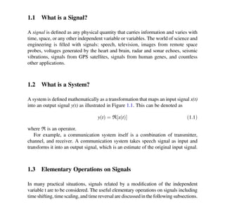
1. Chapter 1
Introduction
1.1 What is a Signal?
A signal is defined as any physical quantity that carries information and varies with
time, space, or any other independent variable or variables. The world of science and
engineering is filled with signals: speech, television, images from remote space
probes, voltages generated by the heart and brain, radar and sonar echoes, seismic
vibrations, signals from GPS satellites, signals from human genes, and countless
other applications.
1.2 What is a System?
A system is defined mathematically as a transformation that maps an input signal x(t)
into an output signal y(t) as illustrated in Figure 1.1. This can be denoted as
y t
ð Þ ¼ ℜ x t
ð Þ
½ ð1:1Þ
where ℜ is an operator.
For example, a communication system itself is a combination of transmitter,
channel, and receiver. A communication system takes speech signal as input and
transforms it into an output signal, which is an estimate of the original input signal.
1.3 Elementary Operations on Signals
In many practical situations, signals related by a modification of the independent
variable t are to be considered. The useful elementary operations on signals including
time shifting, time scaling, and time reversal are discussed in the following subsections.
© Springer International Publishing AG, part of Springer Nature 2018
K. D. Rao, Signals and Systems, https://doi.org/10.1007/978-3-319-68675-2_1
1

2. 1.3.1 Time Shifting
Consider a signal x(t). If it is time shifted by t0, the time-shifted version of x(t) is
represented by x(t t0). The two signals x(t) and x(t t0) are identical in shape but
time shifted relative to each other. If t0 is positive, the signal x(t) is delayed (right
shifted) by t0. If t0 is negative, the signal is advanced (left shifted) by t0. Signals
related in this fashion arise in applications such as sonar, seismic signal processing,
radar, and GPS. The time shifting operation is illustrated in Figure 1.2. If the signal x
(t) shown in Figure 1.2(a) is shifted by t0 ¼ 2 seconds, x(t 2) is obtained as shown
in Figure 1.2(b), i.e., x(t) is delayed (right shifted) by 2 seconds. If the signal is
advanced (left shifted) by 2 seconds, x(t þ 2) is obtained as shown in Figure 1.2(c),
i.e., x(t) is advanced (left shifted) by 2 seconds.
1.3.2 Time Scaling
The compression or expansion of a signal is known as time scaling. The time-scaling
operation is illustrated in Figure 1.3. If the signal x(t) shown in Figure 1.3(a) is
( )
Figure 1.1 Schematic representation of a system
0 2
1
-2 t
x(t)
4
0 2
1
-2 t
x(t-2)
1
-4 0 2
-2 t
x(t+2)
(a) (b)
(c)
Figure 1.2 Illustration of time shifting
2 1 Introduction

3. compressed in time by a factor 2, x(2t) is obtained as shown in Figure 1.3(b). If the
signal x(t) is expanded by a factor of 2, x(t/2) is obtained as shown in Figure 1.3(c).
1.3.3 Time Reversal
The signal x(t) is called the time reversal of the signal x(t). The x(t) is obtained
from the signal x(t) by a reflection about t ¼ 0. The time reversal operation is
illustrated in Figure 1.4. The signal x(t) is shown in Figure 1.4(a), and its time
reversal signal x(t) is shown in Figure 1.4(b).
(a) (b)
-4 -2
-2
2
2
4 t
x(t)
-1
1
-2
-2
2
2
t
x(2t)
-4 -2
-2
2
2
4 t
x(t/2)
Figure 1.3 Illustration of time scaling
t
-2 2
2
x(t)
(a) (b)
t
-2 2
2
x(-t)
Figure 1.4 Illustration of time reversal
1.3 Elementary Operations on Signals 3

4. Example 1.1 Consider the following signals x(t) and xi(t), i ¼ 1,2,3. Express them
using only x(t) and its time-shifted, time-scaled, and time-inverted version.
t
-2
2
x(t)
t
-2 2
2
t
4
4
4
t
2
2
Solution
0
0
0
0 t
2
2
x(t-2)
4
t
2
2
t
2
2
x(-t)
t
-2
2
x(t)
x1 t
ð Þ ¼ x t 2
ð Þ þ x t þ 2
ð Þ
t
2
2
x(-t)
t
-2
2
4 1 Introduction

5. x2 t
ð Þ ¼ x t 2
ð Þ þ x t 2
ð Þ
x3 t
ð Þ ¼ 2x
t
2
2
1.4 Classification of Signals
Signals can be classified in several ways. Some important classifications of signals
are:
1.4.1 Continuous-Time and Discrete-Time Signals
Continuous-time signals are defined for a continuous of values of the independent
variable. In the case of continuous-time signals, the independent variable t is
continuous as shown Figure 1.5(a).
Discrete-time signals are defined only at discrete times, and for these signals, the
independent variable n takes on only a discrete set of amplitude values as shown in
Figure 1.5(b).
1.4.2 Analog and Digital Signals
An analog signal is a continuous-time signal whose amplitude can take any value in
a continuous range. A digital signal is a discrete-time signal that can only have a
discrete set of values. The process of converting a discrete-time signal into a digital
signal is referred to as quantization.
−0.5
0.5
1.5
2.5
3.5
1
2
3
4
0
0 2 4 6 8
Time
a b
Time index n
Amplitude
−0.5
0.5
1.5
2.5
3.5
1
2
3
4
0
Amplitude
10 12 14 16 0 2 4 6 8 10 12 14 16
Figure 1.5 (a) Continuous-time signal, (b) discrete-time signal
1.4 Classification of Signals 5

6. 1.4.3 Periodic and Aperiodic Signals
A signal x(t) is said to be periodic with period T(a positive nonzero value), if it
exhibits periodicity, i.e., x(t þ T) ¼ x(t), for all values of t as shown in Figure 1.6(a).
Periodic signal has the property that it is unchanged by a time shift of T.
A signal that does not satisfy the above periodicity property is called an aperiodic
signal. The signal shown in Figure 1.6(b) is an example of an aperiodic signal.
Example 1.2 For each of the following signals, determine whether it is periodic or
aperiodic. If periodic, find the period.
(i) x(t) ¼ 5 sin(2πt)
(ii) x(t) ¼ 1 þ cos(4t þ 1)
(iii) x(t) ¼ e2t
(iv) x t
ð Þ ¼ ej 5tþπ
2
ð Þ
(v) x t
ð Þ ¼ ej 5tþπ
2
ð Þe2t
Solution
(i) It is periodic signal, period ¼ 2π
2π ¼ 1:
(ii) It is periodic, period ¼ 2π
4 ¼ π
2
(iii) It is aperiodic,
(iv) It is periodic. period ¼ 2π
5
(v) Since x(t) is a complex exponential multiplied by a decaying exponential, it is
aperiodic.
Example 1.3 If a continuous-time signal x(t) is periodic, for each of the following
signals, determine whether it is periodic or aperiodic. If periodic, find the period.
(i) x1(t) ¼ x(2t)
(ii) x2(t) ¼ x(t/2)
Solution Let T be the period of x(t). Then, we have
x t
ð Þ ¼ x t þ T
ð Þ
(a) (b)
0 1
1
2 Time
x(t)
0
−1
0
1
−0.5
0.5
0.05 0.1
Time (sec)
Amplitude
0.2
0.15
Figure 1.6 (a) Periodic signal, (b) aperiodic signal
6 1 Introduction

7. (i) For x1(t) to be periodic,
x 2t
ð Þ ¼ x 2t þ T
ð Þ
x 2t þ T
ð Þ ¼ x 2 t þ
T
2
¼ x1 t þ
T
2
Since x1 t
ð Þ ¼ x1 t þ T
2
, x1(t) is periodic with fundamental period T
2.
As x1(t) is compressed version of x(t) by half, the period of x1(t) is also com-
pressed by half.
(ii) For x2(t) to be periodic,
x t=2
ð Þ ¼ x
t
2
þ T
x
t
2
þ T
¼ x
1
2
t þ 2T
ð Þ
¼ x2 t þ 2T
ð Þ
Since x2(t) ¼ x2(t þ 2T), x2(t) is periodic with fundamental period 2T. As x2(t) is
expanded version of x(t) by two, the period of x2(t) is also twice the period of x(t).
Proposition 1.1 Let continuous-time signals x1(t) and x2(t) be periodic signals with
fundamental periods T1 and T2, respectively. The signal x(t) that is a linear combi-
nation of x1(t) and x2(t) is periodic if and only if there exist integers m and k such that
mT1 ¼ kT2 and
T1
T2
¼
k
m
¼ rational number ð1:2Þ
The fundamental period of x(t) is given by mT1 ¼ kT2 provided that the values of m
and k are chosen such that the greatest common divisor (gcd) between m and k is 1.
Example 1.4 For each of the following signals, determine whether it is periodic or
aperiodic. If periodic, find the period.
(i) x(t) ¼ 2 cos(4πt) þ 3 sin(3πt)
(ii) x(t) ¼ 2 cos(4πt) þ 3 sin(10t)
Solution
(i) Let x1(t) ¼ 2 cos(4πt) and x2(t) ¼ 3 sin(3πt).
The fundamental period of x1(t) is
T1 ¼
2π
4π
¼
1
2
1.4 Classification of Signals 7

8. The fundamental period of x2(t) is
T2 ¼
2π
3π
¼
2
3
The ratio T1
T2
¼ 1=2
2=3 ¼ 3
4 is a rational number. Hence, x(t) is a periodic signal.
The fundamental period of the signal x(t) is 4T1 ¼ 3T2 ¼ 2 seconds.
(ii) Let x1(t) ¼ 2 cos(4πt) and x2(t) ¼ 3 sin(10t).
The fundamental period of x1(t) is
T1 ¼
2π
4π
¼
1
2
The fundamental period of x2(t) is
T2 ¼
2π
10
¼
π
5
The ratio T1
T2
¼ 1=2
π=5 ¼ 5
2π is not a rational number. Hence, x(t) is an aperiodic signal.
Example 1.5 Consider the signals
x1 t
ð Þ ¼ cos
2πt
5
þ 2 sin
8πt
5
x2 t
ð Þ ¼ sin πt
ð Þ
Determine whether x3(t) ¼ x1(t)x2(t) is periodic or aperiodic. If periodic, find the
period.
Solution Decomposing signals x1(t) and x2(t) into sums of exponentials gives
x1 t
ð Þ ¼ 1
2 ej 2πt=5
ð Þ
þ 1
2 ej 2πt=5
ð Þ
þ ej 8πt=5
ð Þ
j ej 8πt=5
ð Þ
j
x2 t
ð Þ ¼
ej πt
ð Þ
2j
ej πt
ð Þ
2j
Then,
x3 t
ð Þ ¼
1
4j
ej 7πt=5
ð Þ
1
4j
ej 3πt=5
ð Þ
þ
1
4j
ej 3πt=5
ð Þ
1
4j
ej 7πt=5
ð Þ
ej 13πt=5
ð Þ
2
þ
ej 3πt=5
ð Þ
2
þ
ej 3πt=5
ð Þ
2
ej 13πt=5
ð Þ
2
It is seen that all complex exponentials are powers of ej(π/5)
. Hence, it is periodic.
Period is 2π
π=5 ¼ 10seconds:
8 1 Introduction

9. 1.4.4 Even and Odd Signals
The continuous-time signal is said to be even when x(t) ¼ x(t). The continuous-
time signal is said to be odd when x(t) ¼ x(t). Odd signals are also known as
nonsymmetrical signals. Examples of even and odd signals are shown in Figure 1.7
(a) and Figure 1.7(b), respectively.
Any signal can be expressed as sum of its even and odd parts as
x t
ð Þ ¼ xe t
ð Þ þ xo t
ð Þ ð1:3Þ
The even part and odd part of a signal are
xe t
ð Þ ¼
x t
ð Þ þ x t
ð Þ
2
ð1:3aÞ
xo t
ð Þ ¼
x t
ð Þ x t
ð Þ
2
ð1:3bÞ
Some important properties of even and odd signals are:
(i) Multiplication of an even signal by an odd signal produces an odd signal.
Proof Let y(t) ¼ xe(t)xo(t)
y t
ð Þ ¼ xe t
ð Þxo t
ð Þ
¼ xe t
ð Þxo t
ð Þ ¼ y t
ð Þ
ð1:4Þ
Hence, y(t) is an odd signal.
(ii) Multiplication of an even signal by an even signal produces an even signal.
Proof Let y(t) ¼ xe(t)xe(t)
y t
ð Þ ¼ xe t
ð Þxe t
ð Þ
¼ xe t
ð Þxe t
ð Þ ¼ y t
ð Þ
ð1:5Þ
Hence, y(t) is an even signal.
0 b
A
-b t
x(t)
(a) (b)
A
x(t)
0 b
-A
-b t
Figure 1.7 (a) Even signal, (b) odd signal
1.4 Classification of Signals 9

10. (iii) Multiplication of an odd signal by an odd signal produces an even signal.
Proof Let y(t) ¼ xo(t)xo(t)
y t
ð Þ ¼ x0 t
ð Þxo t
ð Þ
¼ xo t
ð Þ
ð Þ xo t
ð Þ
ð Þ
¼ xo t
ð Þxo t
ð Þ
¼ y t
ð Þ
Hence, y(t) is an even signal.
It is seen from Figure 1.7(a) that the even signal is symmetric about the vertical
axis, and hence
ð b
b
xe t
ð Þdt ¼ 2
ðb
0
xe t
ð Þdt ð1:6Þ
From Figure 1.6(b), it is also obvious that
ð b
b
xo t
ð Þdt ¼ 0 ð1:7Þ
Eqs. (1.6) and (1.7) are valid for no impulse or its derivative at the origin. These
properties are proved to be useful in many applications.
Example 1.6 Find the even and odd parts of x(t) ¼ ej2t
.
Solution From Eq. (1.3),
ej2t
¼ xe t
ð Þ þ xo t
ð Þ
where
xe t
ð Þ ¼
x t
ð Þ þ x t
ð Þ
2
¼
ej2t
þ ej2t
2
¼ cos 2t
ð Þ
xo t
ð Þ ¼
x t
ð Þ x t
ð Þ
2
¼
ej2t
ej2t
2
¼ j sin 2t
ð Þ:
Example 1.7 If xe(t) and xo(t) are the even and odd parts of x(t), show that
ð1
1
x2
t
ð Þdt ¼
ð1
1
x2
e t
ð Þdt þ
ð1
1
x2
o t
ð Þdt ð1:8Þ
10 1 Introduction

11. Solution ð1
1
x2
t
ð Þdt ¼
ð1
1
xe t
ð Þ þ xo t
ð Þ
ð Þ2
dt
¼
ð1
1
x2
e t
ð Þdt þ 2
ð1
1
xe t
ð Þxo t
ð Þdt þ
ð1
1
x2
o t
ð Þdt
¼
ð1
1
x2
e t
ð Þdt þ
ð1
1
x2
o t
ð Þdt
Since 2
ð1
1
xe t
ð Þxo t
ð Þdt ¼ 0
Example 1.8 For each of the following signals, determine whether it is even, odd,
or neither (Figure 1.8)
Solution By definition a signal is even if and only if x(t) ¼ x(t), while a signal is
odd if and only if x(t) ¼ x(t).
(a) It is readily seen that x(t) 6¼ x(t) for all t and x(t) 6¼ x(t) for all t; thus x(t) is
neither even nor odd.
(b) Since x(t) is symmetric about t ¼ 0, x(t) is even.
(c) Since x(t) ¼ x(t), x(t) is odd in this case.
-4 -2 2
2
4
x(t)
t
-2 2
2
x(t)
(a) (b)
(c)
-2
-2
2
2
x(t)
tt
Figure 1.8 Signals of example 1.8
1.4 Classification of Signals 11

12. 1.4.5 Causal, Noncausal, and Anticausal Signal
A causal signal is one that has zero values for negative time, i.e., t 0. A signal is
noncausal if it has nonzero values for both the negative and positive times. An
anticausal signal has zero values for positive time, i.e., t 0. Examples of causal,
noncausal, and anticausal signals are shown in Figure 1.9(a), 1.9(b), and 1.9(c),
respectively.
Example 1.9 Consider the following noncausal continuous-time signal. Obtain its
realization as causal signal.
-0.5
0.5
x(t)
1
1
-1
t
0
Solution
0
0.5
1.5
x(t)
2
1
-1
t
x(t)
t
x(t)
t
t
x(t)
(a) (b) (c)
Figure 1.9 (a) Causal signal, (b) noncausal signal, (c) anticausal signal
12 1 Introduction

13. 1.4.6 Energy and Power Signals
A signal x(t) with finite energy, which means that amplitude ! 0 as time ! 1, is
said to be energy signal, whereas a signal x(t) with finite and nonzero power is said to
be power signal. The instantaneous power p(t) of a signal x(t) can be expressed by
p t
ð Þ ¼ x2
t
ð Þ ð1:9Þ
The total energy of a continuous-time signal x(t) can be defined as
E ¼
ð1
1
x2
t
ð Þdt ð1:10aÞ
for a complex valued signal
E ¼
ð1
1
x t
ð Þ
j j2
dt ð1:10bÞ
Since the power is the time average of energy, the average power is defined as
P ¼ limT!1
1
T
ðT=2
T=2
x2
t
ð Þdt. The signal x(t) expressed by Eq. (1.11), which is
shown in Figure 1.10(a), is an example of energy signal.
x t
ð Þ ¼
t 0 t 1
1 1 t 2
(
ð1:11Þ
The energy of the signal is given by
E ¼
ð1
1
x2
t
ð Þdt ¼
ð1
0
t2
dt þ
ð2
1
1dt ¼
1
3
þ 1 ¼
4
3
The signal x(t) shown in Figure 1.10(b) is an example of a power signal. The
signal is periodic with period 2. Hence, averaging x2
(t) over infinitely large time
interval is the same as averaging over one period, i.e., 2. Thus, the average power P is
P ¼
1
2
ð1
1
x2
t
ð Þdt ¼
1
2
ð1
1
4t2
dt ¼
4
3
0 1
1
2 Time
x(t)
Figure 1.10(a) Energy
signal
1.4 Classification of Signals 13

14. Thus, an energy signal has finite energy and zero average power, whereas a power
signal has finite power and infinite energy.
Example 1.10 Compute energy and power for the following signals, and determine
whether each signal is energy signal, power signal, or neither.
(i) x(t) ¼ 4sin(2πt), 1 t 1.
(ii) x(t) ¼ 2e2|t|
, 1 t 1.
(iii) x t
ð Þ ¼
2
ffiffi
t
p t 1
0 t 1:
8
:
(iv) x(t) ¼ eat
for real value of a
(v) x(t) ¼ cos (t)
(vi) xðtÞ ¼ ej 2tþ
π
4Þ
ð
Solution
(i)
E ¼
ð1
1
x t
ð Þ
j j2
dt ¼
ð1
1
4 sin 2πt
ð Þ
j j2
dt
¼ 16
ð1
1
1 cos 4πt
ð Þ
2
dt
¼ 16
ð1
1
1
2
dt 8
ð1
1
cos 4πt
ð Þdt
¼ 1
P ¼ limT!1
1
T
ðT=2
T=2
x2
ðtÞdt ¼ limT!1
1
T
ðT=2
T=2
16 sin 2
ð2πtÞdt
¼ limT!1
1
T
ðT=2
T=2
16
1 cos ð4πtÞ
2
dt
¼ 16 limT!1
1
T
ðT=2
T=2
1
2
dt 16 limT!1
1
T
ðT=2
T=2
cos ð4πtÞ
2
dt
¼ 8
-4 -2
-2
2
2
4 t
x(t)
Figure 1.10(b) Power
signal
14 1 Introduction

15. The energy of the signal is infinite, and its average power is finite; x(t) is a power
signal.
(ii) x(t) ¼ 2e2|t|
E ¼
ð1
1
x t
ð Þ
j j2
dt ¼
ð1
1
2e2 t
j j 2
dt
¼ 4
ð0
1
e4t
dt þ 4
ð1
0
e4t
dt
¼
4
4
e4t 0
1
þ
4
4
e4t 1
0
¼
4
4
þ
4
4
¼ 2
P ¼ limT!1
1
T
ðT=2
T=2
x2
t
ð Þdt ¼ limT!1
1
T
ðT=2
T=2
2e2 t
j j 2
dt
¼ 4 limT!1
1
T
ð0
T=2
e4t
dt þ 4 limT!1
1
T
ðT=2
0
e4t
dt
¼
4
4
limT!1
1
T
e4t 0
T=2
þ
4
4
limT!1
1
T
e4t T=2
0
¼
4
4
limT!1
1
T
1 e2T
þ
4
4
limT!1
1
T
e2T
1
¼ 0 þ 0 ¼ 0
The energy of the signal is finite, and its average power is zero; x(t) is an energy
signal.
(iii) x t
ð Þ ¼
2
ffiffi
t
p t 1
0 t 1:
8
:
E ¼
ð1
1
x t
ð Þ
j j2
dt ¼
ð1
1
4
t
dt
¼ 4ln t
½ 1
1
¼ 1
1.4 Classification of Signals 15

16. P ¼ lim
T!1
1
T
ðT=2
T=2
x2
t
ð Þdt ¼ lim
T!1
1
T
ðT=2
1
4
t
dt
¼ 4 lim
T!1
1
T
ln t
½
1T=2
¼ 4 lim
T!1
1
T
ln
T
2
1
T
ln 1
½
¼ 4 lim
T!1
1
T
ln
T
2
¼ 4 lim
T!1
ln
T
2
T
0
B
B
@
1
C
C
A
Using L’Hospital’s rule, we see that the power of the signal is zero. That is
P ¼ 4 lim
T!1
ln T
2
T
¼ 4 lim
T!1
2
T
1
¼ 0
The energy of the signal is infinite and its average power is zero; x(t) is neither
energy signal nor power signal.
(iv) x(t) ¼ eat
for real value of a
E ¼
ð1
1
x t
ð Þ
j j2
dt ¼
ð1
1
eat
j j
2
dt ¼ 1,
P ¼ limT!1
1
T
ðT=2
T=2
x2
t
ð Þdt ¼ limT!1
1
T
ðT=2
T=2
e2at
dt
¼ lim
T!1
eaT
eaT
2aT
¼ lim
T!1
eaT
2aT
lim
T!1
eaT
2aT
¼ lim
T!1
eaT
2aT
0
Using L’Hospital’s rule, we see that the power of the signal is infinite. That is,
P ¼ lim
T!1
eaT
2aT
¼ lim
T!1
eaT
2
¼ 1
The energy of the signal is infinite and its average power is infinite; x(t) is neither
energy signal nor power signal.
(v) x(t) ¼ cos(t)
E ¼
ð1
1
x t
ð Þ
j j2
dt ¼
ð1
1
cos 2
t
ð Þdt ¼ 1,
16 1 Introduction

17. P ¼ limT!1
1
T
ðT=2
T=2
x2
t
ð Þdt ¼ limT!1
1
T
ðT=2
T=2
cos 2
t
ð Þdt
¼ limT!1
1
T
ðT=2
T=2
1 þ cos 2t
ð Þ
2
dt
¼ limT!1
1
T
ðT=2
T=2
1
2
dt þ limT!1
1
T
ðT=2
T=2
cos 2t
ð Þ
2
dt
¼
1
2
The energy of the signal is infinite and its average power is finite; x(t) is a power
signal.
(vi) x t
ð Þ ¼ ej 2tþπ
4
ð Þ, x t
ð Þ
j j ¼ 1.
E ¼
ð1
1
x t
ð Þ
j j2
dt ¼
ð1
1
dt ¼ 1,
P ¼ limT!1
1
T
ðT=2
T=2
x2
t
ð Þdt ¼ limT!1
1
T
ðT=2
T=2
1dt ¼ limT!11 ¼ 1
The energy of the signal is infinite and its average power is finite; x(t) is a power
signal.
Example 1.11 Consider the following signals, and determine the energy of each
signal shown in Figure 1.11. How does the energy change when transforming a
signal by time reversing, sign change, time shifting, or doubling it?
t
2
2
x(t)
t
-2
2
(t)
4
t
2
2
( )
t
2
-2
(t)
t
2
4
( )
Figure 1.11 Signals of example 1.11
1.4 Classification of Signals 17

18. Solution
xðtÞ ¼
(
t 0 t 2
0 otherwise
Ex ¼
ð1
1
jxðtÞj2
dt ¼
ð2
0
t2
dt ¼
t3
3
2
0
¼
8
3
x1ðtÞ ¼
(
t 2 t 0
0 otherwise
Ex1
¼
ð1
1
jx1ðtÞj2
dt ¼
ð0
2
t2
dt ¼
t3
3
0
2
¼
8
3
x2ðtÞ ¼
(
t 0 t 2
0 otherwise
Ex2
¼
ð1
1
jx2ðtÞj2
dt ¼
ð2
0
t2
dt ¼
t3
3
2
0
¼
8
3
x3ðtÞ ¼
(
ðt 2Þ 2 t 4
0 otherwise
Ex3
¼
ð1
1
jx3ðtÞj2
dt ¼
ð2
0
ðt 2Þ2
dt ¼
ð4
2
ðt2
4t þ 4Þdt
¼
t3
3
2t2
þ 4t
4
2
¼
8
3
x4ðtÞ ¼
(
2t 0 t 2
0 otherwise
Ex4
¼
ð1
1
jx4ðtÞj2
dt ¼
ð2
0
4t2
dt ¼ 4
t3
3
2
0
¼
32
3
The time reversal, sign change, and time shifting do not affect the signal energy.
Doubling the signal quadruples its energy. Similarly, it can be shown that the energy
of k x(t) is k2
Ex.
Proposition 1.2 The sum of two sinusoids of different frequencies is the sum of the
power of individual sinusoids regardless of phase.
Proof Let us consider a sinusoidal signal x(t) ¼ Acos(Ωt + θ). The power of x(t) is
given by
18 1 Introduction

19. P ¼ limT!1
1
T
ðT=2
T=2
x2
ðtÞdt ¼ limT!1
1
T
ðT=2
T=2
A2
cos 2
ðΩt þ θÞdt
¼ limT!1
1
2T
ðT=2
T=2
A2
½1 þ cos 2
ð2Ωt þ 2θÞdt
¼ limT!1
A2
2T
ðT=2
T=2
dt þ
ðT=2
T=2
cos 2Ωt þ 2θ
ð Þdt
#
¼
A2
2T
½T þ 0 ¼
A2
2
ð1:12Þ
Thus, a sinusoid signal of amplitude A has a power A2
2 regardless of the values of
its frequency Ω and phase θ.
Now, consider the following two sinusoidal signals:
x1 t
ð Þ ¼ A1 cos Ω1t þ θ1
ð Þ
x2 t
ð Þ ¼ A2 cos Ω2t þ θ2
ð Þ
Let xs t
ð Þ ¼ x1 t
ð Þ þ x2 t
ð Þ
The power of the sum of the two sinusoidal signals is given by
Ps ¼ limT!1
1
T
ðT
2
T
2
x2
s ðtÞ
¼ limT!1
1
T
ðT=2
T=2
½A1cos ðΩ1t þ θ1Þ þ A2cos ðΩ2t þ θ2Þ2
dt
¼ limT!1
1
T
ðT
2
T
2
A2
1cos 2
ðΩ1t þ θ1Þdt
þ limT!1
1
T
ðT
2
T
2
A2
2cos 2
ðΩ2t þ θ2Þdt
þ limT!1
2A1A2
T
ðT
2
T
2
cos ðΩ1t þ θ1Þcos ðΩ2t þ θ2Þdt
The first and second integrals on the right-hand side are the powers of the two
sinusoidal signals, respectively, and the third integral becomes zero since
cos Ω1t þ θ1
ð Þ cos Ω2t þ θ2
ð Þ ¼ cos Ω1 þ Ω2
ð Þt þ θ1 þ θ2
ð Þ
½
þ cos Ω1 Ω2
ð Þt þ θ1 θ2
ð Þ
½
Hence,
Ps ¼
A2
1
2
þ
A2
2
2
ð1:13Þ
1.4 Classification of Signals 19

20. It can be easily extended to sum of any number of sinusoids with distinct
frequencies
1.4.7 Deterministic and Random Signals
For any given time, the values of deterministic signal are completely specified as
shown in Figure 1.12(a). Thus, a deterministic signal can be described mathemati-
cally as a function of time. A random signal takes random statistically characterized
random values as shown in Figure 1.12(b) at any given time. Noise is a common
example of random signal.
1.5 Basic Continuous-Time Signals
1.5.1 The Unit Step Function
The unit step function is defined as
u t
ð Þ ¼
1 t 0
0 t 0
ð1:14Þ
which is shown in Figure 1.13.
It should be noted that u(t) is discontinuous at t ¼ 0.
1
u(t)
t
Figure 1.13 Unit step
function
1
1
−1
0.5
−0.5
0
0.8
0.6
0.4
0.2
0
0 50
0 0.05 0.15
0.1
Time (sec)
Amplitude
0.2
100 150
(a) (b)
Figure 1.12 (a) Deterministic signal, (b) random signal
20 1 Introduction

21. 1.5.2 The Unit Impulse Function
The unit impulse function also known as the Dirac delta function, which is often
referred as delta function is defined as
δ t
ð Þ ¼ 0, t 6¼ 0 ð1:15aÞ
ð1
1
δ t
ð Þ ¼ 1: ð1:15bÞ
The delta function shown in Figure 1.14(b) can be evolved as the limit of the
rectangular pulse as shown in Figure 1.14(a).
δ t
ð Þ ¼ lim
Δ!0
pΔ t
ð Þ ð1:16Þ
As the width Δ ! 0, the rectangular function converges to the impulse function
δ(t) with an infinite height at t ¼ 0, and the total area remains constant at one.
Some Special Properties of the Impulse Function
• Sampling property
If an arbitrary signal x(t) is multiplied by a shifted impulse function, the product is
given by
x t
ð Þδ t t0
ð Þ ¼ x t0
ð Þδ t t0
ð Þ ð1:17aÞ
implying that multiplication of a continuous-time signal and an impulse function
produces an impulse function, which has an area equal to the value of the
continuous-time function at the location of the impulse. Also, it follows that for
t0 ¼ 0,
x t
ð Þδ t
ð Þ ¼ x 0
ð Þδ t
ð Þ ð1:17bÞ
• Shifting property
ð1
1
x t
ð Þδ t t0
ð Þdt ¼ x t0
ð Þ ð1:18Þ
pΔ(t)
(a) (b)
1/Δ
Δ/2
−Δ/2
d(t)
t
t
0
Figure 1.14
(a) Rectangular pulse,
(b) unit impulse
1.5 Basic Continuous-Time Signals 21

22. • Scaling property
δ at þ b
ð Þ ¼
1
a
j j
δ t þ
b
a
ð1:19Þ
• The unit impulse function can be obtained by taking the derivative of the unit step
function as follows:
δ t
ð Þ ¼
du t
ð Þ
dt
ð1:20Þ
• The unit step function is obtained by integrating the unit impulse function as
follows:
u t
ð Þ ¼
ð t
1
δ t
ð Þdt ð1:21Þ
1.5.3 The Ramp Function
The ramp function is defined as
r t
ð Þ ¼
t t 0
0 t 0
ð1:22aÞ
which can also be written as
r t
ð Þ ¼ tu t
ð Þ ð1:22bÞ
The ramp function is shown in Figure 1.15.
1.5.4 The Rectangular Pulse Function
The continuous-time rectangular pulse function is defined as
Figure 1.15 The ramp
function
22 1 Introduction

23. x t
ð Þ ¼
1 t
j j T1
0 t
j j T1
ð1:23Þ
which is shown in Figure 1.16.
1.5.5 The Signum Function
The signum function also called sign function is defined as
sgn t
ð Þ ¼
1 t 0
0 t ¼ 0
1 t 0
8
:
ð1:24Þ
which is shown in Figure 1.17.
1.5.6 The Real Exponential Function
A real exponential function is defined as
x t
ð Þ ¼ Aeσt
ð1:25Þ
where both A and σ are real. If σ is positive, x(t) is a growing exponential signal. The
signal x(t) is exponentially decaying for negative σ. For σ ¼ 0, the signal x(t) is equal
to a constant. Exponentially decaying signal and exponentially growing signal are
shown in Figure 1.18(a) and (b), respectively.
0
1
1
-
1 t
x(t)
Figure 1.16 The
rectangular pulse function
-1
0
1
t
x(t)=
Figure 1.17 The signum
function
1.5 Basic Continuous-Time Signals 23

24. 1.5.7 The Complex Exponential Function
A real exponential function is defined as
x t
ð Þ ¼ Ae σþjΩ
ð Þt
ð1:26Þ
Hence
x t
ð Þ ¼ Aeσt
ejΩt
ð1:26aÞ
Using Euler’s identity
ejΩt
¼ cos Ωt
ð Þ þ j sin Ωt
ð Þ ð1:27Þ
Substituting Eq. (1.27) in Eq. (1.26a), we obtain
x t
ð Þ ¼ Aeσt
cos Ωt
ð Þ þ j sin Ωt
ð Þ
ð Þ ð1:28Þ
Real sine function and real cosine function can be expressed by the trigonometric
identities as
cos Ωt
ð Þ ¼ ejΩt
þejΩt
2 and sin Ωt
ð Þ ¼ ejΩt
ejΩt
2j
1.5.8 The Sinc Function
The continuous-time sinc function is defined as
Sinc t
ð Þ ¼
sin πt
ð Þ
πt
ð1:28Þ
which is shown in Figure 1.19
A
0
t
x(t)
A
0
t
x(t)
(a) (b)
Figure 1.18 Real exponential function. (a) Decaying, (b) growing
24 1 Introduction

25. Example 1.12 State whether the following signals are causal, anticausal, or
noncausal.
(a) x(t) ¼ e2t
u(t)
(b) x(t) ¼ tu(t) t(u(t 1) þ e(1t)
u(t 1))
(c) x(t) ¼ et
cos (2πt)u(1 t)
Solution (a)
1
0.25
x(t)
1
t
It is causal since x(t) ¼ 0 for t 0
(b)
1
1
t
x(t)
It is causal since x(t) ¼ 0 for t 0
Figure 1.19 The sinc function
1.5 Basic Continuous-Time Signals 25

26. (c)
(c )
It is non causal since for t0
u(1-t)
1
t
Example 1.13 Determine and plot the even and odd components of the following
continuous-time signal
x t
ð Þ ¼ tu t þ 2
ð Þ tu t 1
ð Þ
Solution
x t
ð Þ ¼ tu t þ 2
ð Þ tu t 1
ð Þ
x t
ð Þ ¼ tu t þ 2
ð Þ þ tu t þ 1
ð Þ
-2
-2 1
x(t)
1
t 2
-2
-2 1
x(-t)
1
t
xeðtÞ ¼
xðtÞ þ xðtÞ
2
¼
1
2
t
uðt þ 2Þ uðt 1Þ uðt þ 2Þ þ uðt þ 1Þ
26 1 Introduction

27. -0.5
2
-1
-2
1
1
)
(
t
xo t
ð Þ ¼
x t
ð Þ x t
ð Þ
2
¼
1
2
t u t þ 2
ð Þ u t 1
ð Þ þ u t þ 2
ð Þ u t þ 1
ð Þ
ð Þ
-0.5
2
-1
-2
1
1
t
Example 1.14 Simplify the following expressions:
(a) sin t
t2þ3
δ t
ð Þ
(b) 4þjt
3jt δ t 1
ð Þ
(c)
Ð1
1 4t 3
ð ÞÞδ t 1
ð Þdt
Solution
(a) sin 0
ð Þ
0þ3
δ t
ð Þ ¼ 0
(b) 4þjt
3jt δ t 1
ð Þ ¼ 4þj
3j δ t 1
ð Þ
(c)
Ð1
1 4 1
ð Þ 3
ð ÞÞδ t 1
ð Þdt ¼
Ð1
1 1δ t 1
ð Þdt ¼ 1:
1.5 Basic Continuous-Time Signals 27

28. 1.6 Generation of Continuous-Time Signals Using
MATLAB
An exponentially damped sinusoidal signal can be generated using the following
MATLAB command:
x(t) ¼ A ∗ sin (2 ∗ pi ∗ f0 ∗ t + θ) ∗ exp (a ∗ t)where a is positive for
decaying exponential.
Example 1.15 Write a MATLAB program to generate the following exponentially
damped sinusoidal signal.
x(t) ¼ 5 sin (2πt)e0.4t
10 t 10
Solution The following MATLAB program generates the exponentially damped
sinusoidal signal as shown in Figure 1.20.
MATLAB program to generate exponentially damped sinusoidal signal
clear all;clc;
x =inline('5*sin(2*pi*1*t).*exp(-.4*t)','t');
t = (-10:.01:10);
plot(t,x(t));
xlabel ('t (seconds)');
ylabel ('Ámplitude');
-10 -8 -6 -4 -2 0 2 4 6 8 10
-250
-200
-150
-100
-50
0
50
100
150
200
250
t (seconds)
Ámplitude
Figure 1.20 Exponentially damped sinusoidal signal with exponential parameter a ¼ 0.4.
28 1 Introduction

29. Example 1.16 Generate unit step function over [5,5] using MATLAB
Solution The following MATLAB program generates the unit step function over
[5,5] as shown in Figure 1.21.
MATLAB program to generate unit step function over [5,5]
clear all;clc;
u=inline('(t=0)','t');
t=-5:0.01:5;
plot(t,u(t))
xlabel ('t (seconds)');
ylabel ('Ámplitude')
axis([-5 5 -2 2])
Example 1.17 Generate the following rectangular pulse function rect(t) using
MATLAB:
rect t
10
¼
1, 5 t 5
0, elsewhere
Solution The following MATLAB program generates the rectangular pulse func-
tion as shown in Figure 1.22.
-5 -4 -3 -2 -1 0 1 2 3 4 5
-2
-1.5
-1
-0.5
0
0.5
1
1.5
2
t (seconds)
Ámplitude
Figure 1.21 Unit step function
1.6 Generation of Continuous-Time Signals Using MATLAB 29

30. MATLAB program to generate rectangular pulse function
clear all;clc;
u=inline('(t=-5) (t5)','t');
t=-10:0.01:10;
plot(t,u(t))
xlabel ('t (seconds)');
ylabel ('Ámplitude')
axis([-10 10 -2 2])
1.7 Typical Signal Processing Operations
1.7.1 Correlation
Correlation of signals is necessary to compare one reference signal with one or more
signals to determine the similarity between them and to determine additional infor-
mation based on the similarity. Applications of cross correlation include cross-
spectral analysis, detection of signals buried in noise, pattern matching, and delay
measurements.
-10 -8 -6 -4 -2 0 2 4 6 8 10
-2
-1.5
-1
-0.5
0
0.5
1
1.5
2
t (seconds)
Ámplitude
Figure 1.22 Rectangular pulse function
30 1 Introduction

31. 1.7.2 Filtering
Filtering is basically a frequency domain operation. Filter is used to pass certain band
of frequency components without any distortion and to block other frequency
components. The range of frequencies that is allowed to pass through the filter is
called the passband, and the range of frequencies that is blocked by the filter is called
the stopband. A low-pass filter passes all low-frequency components below a certain
specified frequency Ωc, called the cutoff frequency, and blocks all high-frequency
components above Ωc. A high-pass filter passes all high-frequency components
above a certain cutoff frequency Ωc and blocks all low-frequency components
below Ωc. A band-pass filter passes all frequency components between two cutoff
frequencies Ωc1 and Ωc2 where Ωc1 Ωc2 and blocks all frequency components
below the frequency Ωc1 and above the frequency Ωc2. A band-stop filter blocks all
frequency components between two cutoff frequencies Ωc1 and Ωc2 where Ωc1 Ωc2
and passes all frequency components below the frequency Ωc1 and above the
frequency Ωc2. Notch filter is a narrow band-stop filter used to suppress a particular
frequency, called the notch frequency.
1.7.3 Modulation and Demodulation
Transmission media, such as cables and optical fibers, are used for transmission of
signals over long distances; each such medium has a bandwidth that is more suitable
for the efficient transmission of signals in the high-frequency range. Hence, for
transmission over such channels, it is necessary to transform the low-frequency
signal to a high-frequency signal by means of a modulation operation. The desired
low-frequency signal is extracted by demodulating the modulated high-frequency
signal at the receiver end.
1.7.4 Transformation
The transformation is the representation of signals in the frequency domain, and
inverse transform converts the signals from the frequency domain back to the time
domain. The transformation provides the spectrum analysis of a signal. From the
knowledge of the spectrum of a signal, the bandwidth required to transmit the signal
can be determined. The transform domain representations provide additional insight
into the behavior of the signal and make it easy to design and implement algorithms,
such as those for filtering, convolution, and correlation.
1.7 Typical Signal Processing Operations 31

32. 1.7.5 Multiplexing and Demultiplexing
Multiplexing is used in situations where the transmitting media is having higher
bandwidth, but the signals have lower bandwidth. Thus, multiplexing is the process
in which multiple signals, coming from different sources, are combined and trans-
mitted over a single channel. Multiplexing is performed by multiplexer placed at the
transmitter end. At the receiving end, the composite signal is separated by demul-
tiplexer performing the reverse process of multiplexing and routes the separated
signals to their corresponding receivers or destinations.
In electronic communications, the two basic forms of multiplexing are time-
division multiplexing (TDM) and frequency-division multiplexing (FDM). In
time-division multiplexing, transmission time on a single channel is divided into
non-overlapped time slots. Data streams from different sources are divided into units
with same size and interleaved successively into the time slots. In frequency-division
multiplexing (FDM), numerous low-frequency narrow bandwidth signals are com-
bined for transmission over a single communication channel. A different frequency
is assigned to each signal within the main channel. Code-division multiplexing
(CDM) is a communication networking technique in which multiple data signals
are combined for simultaneous transmission over a common frequency band.
1.8 Some Examples of Real-World Signals and Systems
1.8.1 Audio Recording System
An audio recording system shown in Figure 1.23(a) takes an audio or speech as input
and converts the audio signal into an electrical signal, which is recorded on a
magnetic tape or a compact disc. An example of recorded voice signal is shown in
Figure 1.23(b).
(a) (b)
Audio
output
signal
Audio
Recording
System
Figure 1.23 (a) Audio recording system, (b) the recorded voice signal “don’t fail me again”
32 1 Introduction