This document discusses adaptive filtering, which uses an iterative method to automatically adjust filter coefficients over time to deal with non-stationary signals. It describes the general adaptive filtering block diagram and algorithm. It then discusses specific applications of adaptive filtering, including adaptive frequency estimation/system identification, adaptive noise cancelling, and adaptive line enhancement. It provides an example of using adaptive filtering for system identification and shows the results of the first three iterations.

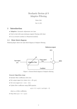
1. Stochastic Section # 9
Adaptive Filtering
Eslam Adel
May 21, 2018
1 Introduction
• Adaptive: Automatic adjustment over time.
• Used to deal with none-stationary signals (Varying with time)
• It is an iterative method or (Numerical method).
1.1 Main block diagram
Following figure shows the main block diagram of adaptive filtering.
Figure 1: General block diagram of adaptive filtering
General Algorithm steps
• Initialize filter coefficients with zeros
• Get output signal ˆx(n) where ˆx(n) = H ∗ y(n)
• Get error signal e(n) = x(n) − ˆx(n)
• Update filter coefficients using LMS equation
ak(n + 1) = ak(n) + µe(n)y(n − k)
where ak is filter coefficients.
• Stop when ak(n + 1) ∼ ak(n)
1

2. 2 Adaptive Frequency Estimation (System identification)
Objective
Identify system or estimate its frequency response. The configuration is a special case from the general config-
uration as follow. see figure 2
• We have unknown system i.e its frequency response is unknown.
• The process can be considered as a calibration of the unknown system till finding its response.
• After convergence, adaptive filter coefficients will be almost the same coefficients of the unknown system
as error almost goes to zero. So we have identified the system.
Figure 2: Adaptive filters for frequency estimation or system identification
3 Adaptive Noise cancelling
Objective: Cancelling the noise and getting the desired signal from noisy one.
The configuration of adaptive noise canceller is shown in figure 3.
Figure 3: Adaptive noise canceller configuration
• We assume that our signal x(n) has two components s(n) and y1(n) i.e x(n) = s(n) + y1(n).
• We have a similar noise signal y2(n).
• Adaptive filter gives us an estimate (ˆy1(n)) of the noise component y1(n).
• Subtracting the estimated signal ˆy1(n) from signal x(n) gives us an estimate of the desired signal ˆs(n).
2

3. 4 Adaptive Line Enhancement
• Adaptive line enhancer is a special case of adaptive noise canceller.
• Only source signal is available and no information about noise component.
• Noise will be same in both versions of signal (Original and delayed one) and adaptive filter will remove
this correlation and cancel the noise.
Figure 4: Adaptive Line enhancer configuration
5 Example
For system identification configuration figure 2. Given
x(n) = [−1, −1.5, −0.5, 0.5, 1.5, 1]
And
y(n) = [−2, −1, 0, 1, 2]
Assuming first order filter H = a0 +a1z−1
and initial values are a0 = 0.2, a1 = 0.3. Adaptation step µ = 0.2.
Identify the unknown system (using three iterations).
Solution
At first Make sure that signals are zero mean, if not subtract the mean. Here our signals are zero mean.
Algorithm steps
• Initialize filter coefficients
• Get output signal ˆx(n) where ˆx(n) = H ∗ y(n).
For first order filter ˆx(n) = a0y(n) + a1y(n − 1)
• Get error signal e(n) = x(n) − ˆx(n)
• Update filter coefficients using LMS equation
a0(n + 1) = a0(n) + 0.2 ∗ e(n)y(n).
a1(n + 1) = a1(n) + 0.2 ∗ e(n)y(n − 1).
Solution is shown is table 1.
Solution is obtained using following python script. We can see that the error is decreasing and values of our
filter is converging. Unknown system will the same as our adaptive filter.
3

4. Table 1: Results of first three iteration of adaptive filtering example
Iteration n ˆx(n) e(n) a0(n + 1) a1(n + 1)
1 0 -0.4 -0.6 0.44 0.3
2 1 -1.04 -0.46 0.532 0.484
3 2 -0.484 -0.016 0.532 0.4872
1 #!/ usr / bin /env python3
2 # −∗− coding : utf −8 −∗−
3 ”””
4 Created on Mon May 14 18:36:49 2018
5
6 @author : eslam
7 ”””
8 import numpy as np
9
10 # x(n) s i g n a l
11 x = np . array ([ −1 , −1.5 , −0.5 , 0.5 , 1.5 , 1 ] )
12 # y(n) s i g n a l
13 y = np . array ([ −2 , −1, 0 , 1 , 2 ] )
14
15 #I n i t i a l i z e a0 and a1 with 0.2 and 0.3
16 # We can n i t i a l i z e them with zeros but we need to converge f a s t e r
17 a0 , a1 = 0.2 , 0.3
18 # Adaptation step
19 mu = 0.2
20 # Number of i t e r a t i o n s
21 num iterations = 3
22 # Results of each i t e r a t i o n ( to f i l l the table )
23 r e s u l t s = np . zeros (( num iterations , 4 ) )
24 f o r i in range ( num iterations ) :
25 # Boundary condition
26 i f i == 0:
27 #y[ −1] = 0
28 xhat = a0∗y [ i ]
29 e l s e :
30 #Get estimate of x ( xhat ) using convolution with a0 and a1
31 xhat = a0 ∗y [ i ] + a1 ∗y [ i −1]
32 #Get the e r r o r
33 e = x [ i ] − xhat
34 #Update your f i l t e r c o e f f s
35 a0 = a0 + mu∗e∗y [ i ]
36 #Checking f o r boundary condition
37 i f i !=0:
38 a1 = a1 + mu∗e∗y [ i −1]
39 # Add to r e s u l t s matrix
40 r e s u l t s [ i , : ] = np . array ( [ xhat , e , a0 , a1 ] )
6 Useful Links
• Overview of adaptive filtering
• LMS adaptive filter (Matlab)
4