SlideShare a Scribd company logo
1 of 34
Download to read offline
7
Chapter
Kinematics is the branch of mechanics that studies the motion of a body or a system
of bodies without consideration given to its mass or the forces acting on it. A serial-
link manipulator comprises a chain of mechanical links and joints. Each joint can
move its outward neighbouring link with respect to its inward neighbour. One end of
the chain, the base, is generally fixed and the other end is free to move in space and
holds the tool or end-effector.
Figure 7.1 shows two classical robots that are the precursor to all arm-type robots
today.Each robot has six joints and clearly the pose of the end-effector will be a complex
function of the state of each joint.Section 7.1 describes a notation for describing the link
and joint structure of a robot and Sect. 7.2 discusses how to compute the pose of the end-
effector. Section 7.3 discusses the inverse problem, how to compute the position of each
joint given the end-effector pose. Section 7.4 describes methods for generating smooth
paths for the end-effector. The remainder of the chapter covers advanced topics and
two complex applications: writing on a plane surface and a four-legged walking robot.
7.1 lDescribing a Robot Arm
A serial-link manipulator comprises a set of bodies, called links, in a chain and con-
nected by joints. Each joint has one degree of freedom, either translational (a sliding
or prismatic joint) or rotational (a revolute joint). Motion of the joint changes the
relative angle or position of its neighbouring links. The joints of most common robot
are revolute but the Stanford arm shown in Fig. 7.1b has one prismatic joint.
The joint structure of a robot can be described by a string such as “RRRRRR” for
the Puma and “RRPRRR” for the Stanford arm, where the jth character represents the
type of joint j, either Revolute or Prismatic. A systematic way of describing the geom-
etry of a serial chain of links and joints was proposed by Denavit and Hartenberg in
1955 and is known today as Denavit-Hartenberg notation.
For a manipulator with N joints numbered from 1 to N, there are N + 1 links, num-
bered from 0 to N. Link 0 is the base of the manipulator and link N carries the end-
Robot Arm Kinematics
Take to Kinematics. It will repay you.
It is more fecund than geometry; it adds a fourth dimension to space.
Chebyshev
Fig. 7.1.
a The Puma 560 robot was the
first modern industrial robot
(courtesy Oussama Khatib).
b The Stanford arm was an early
research arm and is unusual
in that it has a prismatic joint
(Stanford University AI Lab 1972;
courtesy Oussama Khatib). Both
arms were designed by robotics
pioneer Victor Scheinman and
both robots can be seen in the
Smithsonian Museum of Ameri-
can History, Washington DC
138
effector or tool. Joint j connects link j − 1 to link j and therefore joint j moves link j.A
link is considered a rigid body that defines the spatial relationship between two
neighbouring joint axes.A link can be specified by two parameters,its length aj and its
twist αj. Joints are also described by two parameters. The link offset dj is the distance
from one link coordinate frame to the next along the axis of the joint.The joint angle θj
is the rotation of one link with respect to the next about the joint axis.
Figure 7.2 illustrates this notation.The coordinate frame {j} is attached to the far (dis-
tal) end of link j.The axis of joint j is aligned with the z-axis.These link and joint param-
eters are known as Denavit-Hartenberg parameters and are summarized in Table 7.1.
Following this convention the first joint, joint 1, connects link 0 to link 1. Link 0 is
the base of the robot. Commonly for the first link d1 = α1 = 0 but we could set d1 > 0
to represent the height of the shoulder joint above the base.In a manufacturing system
the base is usually fixed to the environment but it could be mounted on a mobile base
such as a space shuttle, an underwater robot or a truck.
The final joint,joint Nconnects link N − 1 to link N.Link N is the tool of the robot and
the parameters dN and aN specify the length of the tool and its x-axis offset respectively.
The tool is generally considered to be pointed along the z-axis as shown in Fig. 2.14.
The transformation from link coordinate frame {j − 1} to frame {j} is defined in
terms of elementary rotations and translations as
(7.1)
which can be expanded as
(7.2)
Fig. 7.2.
Definition of standard Denavit
and Hartenberg link parameters.
The colors red and blue denote all
things associated with links j − 1
and j respectively. The numbers
in circles represent the order in
which the elementary trans-
forms are applied
Jacques Denavit and Richard Hartenberg introduced many of the key concepts of kinematics for
serial-link manipulators in a 1955 paper (Denavit and Hartenberg 1955) and their later classic
text Kinematic Synthesis of Linkages (Hartenberg and Denavit 1964).
The 3 × 3 orthonormal matrix is aug-
mented with a zero translational com-
ponent to form a 4 × 4 homogenous
transformation.
Chapter 7 · Robot Arm Kinematics
139
The parameters αj and aj are always constant.For a revolute joint θj is the joint vari-
able and dj is constant,while for a prismatic joint dj is variable,θj is constant and αj = 0.
In many of the formulations that follow we use generalized joint coordinates
For an N-axis robot the generalized joint coordinates q ∈ C where C ⊂ RN is called
the joint space or configuration space. For the common case of an all-revolute robot
C ⊂ SN the joint coordinates are referred to as joint angles. The joint coordinates are
also referred to as the pose of the manipulator which is different to the pose of the
end-effector which is a Cartesian pose ξ ∈ SE(3). The term configuration is shorthand
for kinematic configuration which will be discussed in Sect. 7.3.1.
Within the Toolbox we represent a robot link with a Link object which is created by
>> L = Link([0, 0.1, 0.2, pi/2, 0])
L =
theta=q, d=0.1, a=0.2, alpha=1.571 (R,stdDH)
where the elements of the input vector are given in the order θk, dj, aj, αj. The optional
fifth element σj indicates whether the joint is revolute (σi = 0) or prismatic (σi = 0). If
not specified a revolute joint is assumed.
The displayed values of the Link object shows its kinematic parameters as well as
other status such the fact that it is a revolute joint (the tag R) and that the standard
Denavit-Hartenberg parameter convention is used (the tag stdDH).
Although a value was given for θ it is not displayed – that value simply served
as a placeholder in the list of kinematic parameters.θ is substituted by the joint
variable q and its value in the Link object is ignored. The value will be man-
aged by the Link object.
A Link object has many parameters and methods which are described in the online
documentation, but the most common ones are illustrated by the following examples.
The link transform Eq. 7.2 for q = 0.5 rad is
Table 7.1.
Denavit-Hartenberg parameters:
their physical meaning, symbol
and formal definition
Jacques Denavit (1930–) was born in Paris where he studied for his Bachelor degree before
pursuing his masters and doctoral degrees in mechanical engineering at Northwestern Univer-
sity, Illinois. In 1958 he joined the Department of Mechanical Engineering and Astronautical
Science at Northwestern where the collaboration with Hartenberg was formed. In addition to
his interest in dynamics and kinematics Denavit was also interested in plasma physics and
kinetics. After the publication of the book he moved to Lawrence Livermore National Lab,
Livermore, California, where he undertook research on computer analysis of plasma physics
problems. He retired in 1982.
This is the same concept as was intro-
duced for mobile robots on page 65.
A slightly different notation, modifed
Denavit-Hartenberg notation is dis-
cussed in Sect. 7.5.3.
7.1 · Describing a Robot Arm
140
>> L.A(0.5)
ans =
0.8776 -0.0000 0.4794 0.1755
0.4794 0.0000 -0.8776 0.0959
0 1.0000 0.0000 0.1000
0 0 0 1.0000
is a 4 × 4 homogeneous transformation. Various link parameters can be read or al-
tered, for example
>> L.RP
ans =
R
indicates that the link is prismatic and
>> L.a
ans =
0.2000
returns the kinematic parameter a. Finally a link can contain an offset
>> L.offset = 0.5;
>> L.A(0)
ans =
0.8776 -0.0000 0.4794 0.1755
0.4794 0.0000 -0.8776 0.0959
0 1.0000 0.0000 0.1000
0 0 0 1.0000
which is added to the joint variable before computing the link transform and will be
discussed in more detail in Sect. 7.5.1.
7.2 lForward Kinematics
The forward kinematics is often expressed in functional form
(7.3)
with the end-effector pose as a functionof joint coordinates.Using homogeneoustrans-
formations this is simply the product of the individual link transformation matrices
given by Eq. 7.2 which for an N-axis manipulator is
(7.4)
The forward kinematic solution can be computed for any serial-link manipulator
irrespective of the number of joints or the types of joints. Determining the Denavit-
Hartenberg parameters for each of the robot’s links is described in more detail in
Sect. 7.5.2.
The pose of the end-effector ξE ∼ TE ∈ SE(3) has six degrees of freedom – three in
translation and three in rotation. Therefore robot manipulators commonly have six
joints or degrees of freedom to allow them to achieve an arbitrary end-effector pose.
The overall manipulator transform is frequently written as T6 for a 6-axis robot.
Richard Hartenberg (1907–1997) was born in Chicago and studied for his degrees at the University
of Wisconsin,Madison.He served in the merchant marine and studied aeronautics for two years at
the University of Goettingen with space-flight pioneer Theodor von Karman.He was Professor of
mechanical engineering at Northwestern University where he taught for 56 years. His research in
kinematics led to a revival of interest in this field in the 1960s,and his efforts helped put kinemat-
ics on a scientific basis for use in computer applications in the analysis and design of complex
mechanisms. His also wrote extensively on the history of mechanical engineering.
Chapter 7 · Robot Arm Kinematics
141
7.2.1 lA 2-Link Robot
The first robot that we will discuss is the two-link planar manipulator shown in Fig. 7.3.
It has the following Denavit-Hartenberg parameters
which we use to create a vector of Link objects
Fig. 7.3.
Two-link robot as per
Spong et al. (2006, fig. 3.6, p. 84)
>> L(1) = Link([0 0 1 0]);
>> L(2) = Link([0 0 1 0]);
>> L
L =
theta=q1, d=0, a=1, alpha=0 (R,stdDH)
theta=q2, d=0, a=1, alpha=0 (R,stdDH)
which are passed to the constructor SerialLink
>> two_link = SerialLink(L, 'name', 'two link');
which returns a SerialLink object that we can display
>> two_link
two_link =
two link (2 axis, RR, stdDH)
+---+-----------+-----------+-----------+-----------+
| j | theta | d | a | alpha |
+---+-----------+-----------+-----------+-----------+
| 1| q1| 0| 1| 0|
| 2| q2| 0| 1| 0|
+---+-----------+-----------+-----------+-----------+
grav = 0 base = 1 0 0 0 tool = 1 0 0 0
0 0 1 0 0 0 1 0 0
9.81 0 0 1 0 0 0 1 0
0 0 0 1 0 0 0 1
7.2 · Forward Kinematics
142
This provides a concise description of the robot. We see that it has 2 revolute joints as
indicated by the structure string 'RR', it is defined in terms of standard Denavit-
Hartenberg parameters, that gravity is acting in the default z-direction. The kine-
matic parameters of the link objects are also listed and the joint variables are shown as
variables q1 and q2. We have also assigned a name to the robot which will be shown
whenever the robot is displayed graphically. The script
>> mdl_twolink
performs the above steps and defines this robot in the MATLAB® workspace, creating
a SerialLink object named twolink.
The SerialLink object is key to the operation of the Robotics Toolbox. It has a
great many methods and properties which are illustrated in the rest of this part, and
described in detail in the online documentation. Some simple examples are
>> twolink.n
ans =
2
which returns the number of joints, and
>> links = twolink.links
L =
theta=q1, d=0, a=1, alpha=0 (R,stdDH)
theta=q2, d=0, a=1, alpha=0 (R,stdDH)
which returns a vector of Link objects comprising the robot. We can also make a
copy of a SerialLink object
>> clone = SerialLink(twolink, 'name', 'bob')
clone =
bob (2 axis, RR, stdDH)
+---+-----------+-----------+-----------+-----------+
| j | theta | d | a | alpha |
+---+-----------+-----------+-----------+-----------+
| 1| q1| 0| 1| 0|
| 2| q2| 0| 1| 0|
+---+-----------+-----------+-----------+-----------+
grav = 0 base = 1 0 0 0 tool = 1 0 0 0
0 0 1 0 0 0 1 0 0
9.81 0 0 1 0 0 0 1 0
0 0 0 1 0 0 0 1
which has the name 'bob'.
Now we can put the robot arm to work. The forward kinematics are computed us-
ing the fkine method. For the case where q1 = q2 = 0
>> twolink.fkine([0 0])
ans =
1 0 0 2
0 1 0 0
0 0 1 0
0 0 0 1
the method returns the homogenous transform that represents the pose of the
second link coordinate frame of the robot, T2. For a different configuration the
tool pose is
>> twolink.fkine([pi/4 -pi/4])
ans =
1.0000 0 0 1.7071
0 1.0000 0 0.7071
0 0 1.0000 0
0 0 0 1.0000
By convention, joint coordinates with the Toolbox are row vectors.
Normal to the plane in which the robot
moves.
Link objects are derived from the
MATLAB® handle class and can be
set in place.Thus we can write code like
twolink.links(1).a = 2
to change the kinematic parameter a2.
A unique name is required when mul-
tiple robots are displayed graphically,
see Sect. 7.8 for more details.
Chapter 7 · Robot Arm Kinematics
143
The robot can be visualized graphically
>> twolink.plot([0 0])
>> twolink.plot([pi/4 -pi/4])
as stick figures shown in Fig. 7.4. The graphical representation includes the robot’s
name, the final-link coordinate frame, T2 in this case, the joints and their axes, and a
shadow on the ground plane. Additional features of the plot method such as mul-
tiple views and multiple robots are described in Sect. 7.8 with additional details in the
online documentation.
The simple two-link robot introduced above is limited in the poses that it can achieve
since it operates entirely within the xy-plane, its task space is T ⊂ R2.
7.2.2 lA 6-Axis Robot
Truly useful robots have a task space T ⊂ SE(3) enabling arbitrary position and atti-
tude of the end-effector – the task space has six spatial degrees of freedom: three trans-
lational and three rotational. This requires a robot with a configuration space C ⊂ R6
which can be achieved by a robot with six joints.In this section we will use the Puma 560
as an example of the class of all-revolute six-axis robot manipulators. We define an
instance of a Puma 560 robot using the script
>> mdl_puma560
which creates a SerialLink object, p560, in the workspace
>> p560
p560 =
Puma 560 (6 axis, RRRRRR, stdDH)
Unimation; viscous friction; params of 8/95;
+---+-----------+-----------+-----------+-----------+
| j | theta | d | a | alpha |
+---+-----------+-----------+-----------+-----------+
| 1| q1| 0| 0| 1.571|
| 2| q2| 0| 0.4318| 0|
| 3| q3| 0.15| 0.0203| -1.571|
| 4| q4| 0.4318| 0| 1.571|
| 5| q5| 0| 0| -1.571|
| 6| q6| 0| 0| 0|
+---+-----------+-----------+-----------+-----------+
grav = 0 base = 1 0 0 0 tool = 1 0 0 0
0 0 1 0 0 0 1 0 0
9.81 0 0 1 0 0 0 1 0
0 0 0 1 0 0 0 1
Fig. 7.4. Thetwo-linkrobotintwo
different poses, a the pose (0, 0);
b the pose (ý , −ý). Note the
graphical details. Revolute joints
are indicated by cylinders and the
joint axes are shown as line seg-
ments. The final-link coordinate
frameandashadowontheground
are also shown
TheToolbox has scripts to define a num-
ber of common industrial robots in-
cluding the Motoman HP6, Fanuc 10L,
ABB S4 2.8 and the Stanford arm.
7.2 · Forward Kinematics
144
Note that aj and dj are in SI units which means that the translational part of the for-
ward kinematics will also have SI units.
The script mdl_puma560 also creates a number of joint coordinate vectors in the
workspace which represent the robot in some canonic configurations:
qz (0, 0, 0, 0, 0, 0) zero angle
qr (0, ü, −ü , 0, 0, 0) ready, the arm is straight and vertical
qs (0, 0, −ü , 0, 0, 0) stretch, the arm is straight and horizontal
qn (0, ý , −π, 0, ý, 0) nominal, the arm is in a dextrous working pose
and these are shown graphically in Fig. 7.5. These plots are generated using the plot
method, for example
>> p560.plot(qz)
The Puma 560 robot (Programmable Universal Manipulator for Assembly) shown in Fig. 7.1 was
released in 1978 and became enormously popular. It featured an anthropomorphic design, elec-
tric motors and a spherical wrist which makes it the first modern industrial robot – the archetype
of all that followed.
The Puma 560 catalyzed robotics research in the 1980s and it was a very common laboratory
robot. Today it is obsolete and rare but in homage to its important role in robotics research
we use it here. For our purposes the advantages of this robot are that it has been well studied
and its parameters are very well known – it has been described as the “white rat” of robotics
research.
Most modern 6-axis industrial robots are very similar in structure and can be accomodated
simply by changing the Denavit-Hartenberg parameters. The Toolbox has kinematic models for
a number of common industrial robots including the Motoman HP6, Fanuc 10L, and ABB S4 2.8.
Fig. 7.5. The Puma robot in 4 dif-
ferent poses.a Zero angle;b ready
pose; c stretch; d nominal
Well awayfrom singularities,which will
be discussed in Sect. 7.4.3.
Chapter 7 · Robot Arm Kinematics
145
Forward kinematics can be computed as before
>> p560.fkine(qz)
ans =
1.0000 0 0 0.4521
0 1.0000 0 -0.1500
0 0 1.0000 0.4318
0 0 0 1.0000
which returns the homogeneous transformation corresponding to the end-effector
pose T6. The origin of this frame, the link 6 coordinate frame {6}, is defined as the
point of intersection of the axes of the last 3 joints – physically this point is inside the
robot’s wrist mechanism. We can define a tool transform, from the T6 frame to the
actual tool tip by
>> p560.tool = transl(0, 0, 0.2);
in this case a 200 mm extension in the T6 z-direction. The pose of the tool tip, often
referred to as the tool centre point or TCP, is now
>> p560.fkine(qz)
ans =
1.0000 0 0 0.4521
0 1.0000 0 -0.1500
0 0 1.0000 0.6318
0 0 0 1.0000
The kinematic definition we have used considers that the base of the robot is the inter-
section point of the waist and shoulder axes which is a point inside the structure of the
robot. The Puma 560 robot includes a 30 inch tall pedestal.We can shift the origin of the
robot from the point inside the robot to the base of the pedestal using a base transform
>> p560.base = transl(0, 0, 30*0.0254);
where for consistency we have converted the pedestal height to SI units. Now, with
both base and tool transform, the forward kinematics are
>> p560.fkine(qz)
ans =
1.0000 0 0 0.4521
0 1.0000 0 -0.1500
0 0 1.0000 1.3938
0 0 0 1.0000
and we can see that the z-coordinate of the tool is now greater than before.
We can also do more interesting things, for example
>> p560.base = transl(0,0,3) * trotx(pi);
>> p560.fkine(qz)
ans =
1.0000 0 0 0.4521
0 -1.0000 -0.0000 0.1500
0 0.0000 -1.0000 2.3682
0 0 0 1.0000
which positions the robot’s origin 3 m above the world origin with its coordinate frame
rotated by 180° about the x-axis. This robot is now hanging from the ceiling!
Anthropomorphic means having human-like characteristics. The Puma 560 robot was designed
to have approximately the dimensions and reach of a human worker. It also had a spherical joint
at the wrist just as humans have.
Roboticists also tend to use anthropomorphic terms when describing robots. We use words
like waist, shoulder, elbow and wrist when describing serial link manipulators. For the Puma
these terms correspond respectively to joint 1, 2, 3 and 4–6.
By the mdl_puma560 script.
Alternatively we could change the ki-
nematic parameter d6. The tool trans-
form approach is more general since
thefinallinkkinematicparametersonly
allow setting of d6, a6 and α6 which
provide z-axis translation, x-axis trans-
lation and x-axis rotation respectively.
7.2 · Forward Kinematics
146
The Toolbox supports joint angle time series or trajectories such as
>> q
q =
0 0 0 0 0 0
0 0.0365 -0.0365 0 0 0
0 0.2273 -0.2273 0 0 0
0 0.5779 -0.5779 0 0 0
0 0.9929 -0.9929 0 0 0
0 1.3435 -1.3435 0 0 0
0 1.5343 -1.5343 0 0 0
0 1.5708 -1.5708 0 0 0
where each row represents the joint coordinates at a different timestep and the col-
umns represent the joints. In this case the method fkine
>> T = p560.fkine(q);
returns a 3-dimensional matrix
>> about(T)
T [double] : 4x4x8 (1024 bytes)
where the first two dimensions are a 4 × 4 homogeneous transformation and the third
dimension is the timestep. The homogeneous transform corresponding to the joint
coordinates in the fourth row of q is
>> T(:,:,4)
ans =
1.0000 0.0000 0 0.3820
0.0000 1.0000 -0.0000 -0.1500
0 -0.0000 1.0000 1.6297
0 0 0 1.0000
Creating a trajectory is the topic of Sect. 7.4.
7.3 lInverse Kinematics
We have shown how to determine the pose of the end-effector given the joint coordi-
nates and optional tool and base transforms.A problem of real practical interest is the
inverse problem: given the desired pose of the end-effector ξE what are the required
joint coordinates? For example, if we know the Cartesian pose of an object, what joint
coordinates does the robot need in order to reach it? This is the inverse kinematics
problem which is written in functional form as
(7.5)
Ingeneral this function is not unique and for some classes of manipulator no closed-
form solution exists, necessitating a numerical solution.
7.3.1 lClosed-Form Solution
A necessary condition for a closed-form solution of a 6-axis robot is that the three
wrist axes intersect at a single point. This means that motion of the wrist joints only
changes the end-effector orientation, not its translation. Such a mechanism is known
as a spherical wrist and almost all industrial robots have such wrists.
We will explore inverse kinematics using the Puma robot model
>> mdl_puma560
Generated by the jtraj function,
which is discussed in Sect. 7.4.1.
Chapter 7 · Robot Arm Kinematics
147
At the nominal joint coordinates
>> qn
qn =
0 0.7854 3.1416 0 0.7854 0
the end-effector pose is
>> T = p560.fkine(qn)
T =
-0.0000 0.0000 1.0000 0.5963
-0.0000 1.0000 -0.0000 -0.1501
-1.0000 -0.0000 -0.0000 -0.0144
0 0 0 1.0000
Since the Puma 560 is a 6-axis robot arm with a spherical wrist we use the method
ikine6s to compute the inverse kinematics using a closed-form solution. The re-
quired joint coordinates to achieve the pose T are
>> qi = p560.ikine6s(T)
qi =
2.6486 -3.9270 0.0940 2.5326 0.9743 0.3734
Surprisingly, these are quite different to the joint coordinates we started with. How-
ever if we investigate a little further
>> p560.fkine(qi)
ans =
-0.0000 0.0000 1.0000 0.5963
0.0000 1.0000 -0.0000 -0.1500
-1.0000 0.0000 -0.0000 -0.0144
0 0 0 1.0000
we see that these two different sets of joint coordinates result in the same end-effector
pose and these are shown in Fig. 7.6. The shoulder of the Puma robot is horizontally
offset from the waist, so in one solution the arm is to the left of the waist, in the other
it is to the right. These are referred to as the left- and right-handed kinematic con-
figurations respectively. In general there are eight sets of joint coordinates that give
the same end-effector pose – as mentioned earlier the inverse solution is not unique.
We can force the right-handed solution
>> qi = p560.ikine6s(T, 'ru')
qi =
-0.0000 0.7854 3.1416 0.0000 0.7854 -0.0000
which gives the original set of joint angles by specifying a right handed configuration
with the elbow up.
In addition to the left- and right-handed solutions, there are solutions with the
elbow either up or down, and with the wrist flipped or not flipped. For the Puma 560
robot the wrist joint, θ4, has a large rotational range and can adopt one of two angles
Fig. 7.6. Two solutions to the in-
verse kinematic problem, left-
handed and right-handed solu-
tions. The shadow shows clearly
the two different configurations
Themethodikine6scheckstheDe-
navit-Hartenberg parameters to deter-
mine if the robot meets these criteria.
Morepreciselytheelbowisaboveorbe-
low the shoulder.
7.3 · Inverse Kinematics
148
that differ by π rad. Since most robot grippers have just two fingers, see Fig. 2.14, this
makes no difference in its ability to grasp an object.
The various kinematic configurations are shown in Fig. 7.7. The kinematic con-
figuration returned by ikine6s is controlled by one or more of the character flags:
left or right handed 'l', 'r'
elbow up or down 'u', 'd'
wrist flipped or not flipped 'f', 'n'
Due to mechanical limits on joint angles and possible collisions between links not
all eight solutions are physically achievable. It is also possible that no solution can be
achieved, for example
>> p560.ikine6s( transl(3, 0, 0) )
Warning: point not reachable
ans =
NaN NaN NaN NaN NaN NaN
fails because the arm is simply not long enough to reach this pose.A pose may also be
unachievable due to singularity where the alignment of axes reduces the effective de-
grees of freedom (the gimbal lock problem again). The Puma 560 has a singularity
when q5 is equal to zero and the axes of joints 4 and 6 become aligned. In this case the
best that ikine6s can do is to constrain q4 + q6 but their individual values are arbi-
trary. For example consider the configuration
>> q = [0 pi/4 pi 0.1 0 0.2];
for which q4 + q6 = 0.3. The inverse kinematic solution is
>> p560.ikine6s(p560.fkine(q), 'ru')
ans =
-0.0000 0.7854 3.1416 2.9956 0.0000 -2.6956
Fig. 7.7. Different configurations
of the Puma 560 robot. a Right-
up-noflip; b right-down-noflip;
c right-down-flip
Chapter 7 · Robot Arm Kinematics
149
has quite different values for q4 and q6 but their sum
>> q(4)+q(6)
ans =
0.3000
remains the same.
7.3.2 lNumerical Solution
For the case of robots which do not have six joints and a spherical wrist we need to use
an iterative numerical solution. Continuing with the example of the previous section
we use the method ikine to compute the general inverse kinematic solution
>> T = p560.fkine(qn)
ans =
-0.0000 0.0000 1.0000 0.5963
-0.0000 1.0000 -0.0000 -0.1501
-1.0000 -0.0000 -0.0000 -0.0144
0 0 0 1.0000
>> qi = p560.ikine(T)
qi =
0.0000 -0.8335 0.0940 -0.0000 -0.8312 0.0000
which is different to the original value
>> qn
qn =
0 0.7854 3.1416 0 0.7854 0
but does result in the correct tool pose
>> p560.fkine(qi)
ans =
-0.0000 0.0000 1.0000 0.5963
-0.0000 1.0000 -0.0000 -0.1501
-1.0000 -0.0000 -0.0000 -0.0144
0 0 0 1.0000
Plotting the pose
>> p560.plot(qi)
shows clearly that ikine has found the elbow-down configuration.
A limitation of this general numeric approach is that it does not provide explicit
control over the arm’s kinematic configuration as did the analytic approach – the only
control is implicit via the initial value of joint coordinates (which defaults to zero). If
we specify the initial joint coordinates
>> qi = p560.ikine(T, [0 0 3 0 0 0])
qi =
0.0000 0.7854 3.1416 0.0000 0.7854 -0.0000
the solution converges on the elbow-up configuration.
Aswouldbeexpectedthegeneralnumericalapproachof ikineisconsiderablyslower
than the analytic approach of ikine6s. However it has the great advantage of being
able to work with manipulators at singularities and manipulators with less than six or
more than six joints. Details of the principle behind ikine is provided in Sect. 8.4.
7.3.3 lUnder-Actuated Manipulator
An under-actuated manipulator is one that has fewer than six joints, and is therefore
limitedintheend-effectorposesthatitcanattain.SCARArobotssuchasshownonpage 135
are a common example, they have typically have an x-y-z-θ task space, T ⊂ R3 × S
and a configuration space C ⊂ S3 × R.
7.3 · Inverse Kinematics
Whensolvingforatrajectoryasonp.146
the inverse kinematic solution for one
point is used to initialize the solution
for the next point on the path.
150
We will revisit the two-link manipulator example from Sect. 7.2.1,first defining the robot
>> mdl_twolink
and then defining the desired end-effector pose
>> T = transl(0.4, 0.5, 0.6);
However this pose is over-constrained for the two-link robot – the tool cannot meet
the orientation constraint on the direction of '2 and (2 nor a z-axis translational
value other than zero. Therefore we require the ikine method to consider only er-
ror in the x- and y-axis translational directions, and ignore all other Cartesian de-
grees of freedom.We achieve this by specifying a mask vector as the fourth argument
>> q = twolink.ikine(T, [0 0], [1 1 0 0 0 0])
q =
-0.3488 2.4898
The elements of the mask vector correspond respectively to the three translations
and three orientations: tx, ty, tz, rx, ry, rz in the end-effector coordinate frame. In this
example we specified that only errors in x- and y-translation are to be considered
(the non-zero elements). The resulting joint angles correspond to an endpoint pose
>> twolink.fkine(q)
ans =
ans =
-0.5398 -0.8418 0 0.4000
0.8418 -0.5398 0 0.5000
0 0 1.0000 0
0 0 0 1.0000
which has the desired x- and y-translation, but the orientation and z-translation are
incorrect, as we allowed them to be.
7.3.4 lRedundant Manipulator
A redundant manipulator is a robot with more than six joints. As mentioned previ-
ously, six joints is theoretically sufficient to achieve any desired pose in a Cartesian
taskspace T ⊂ SE(3). However practical issues such as joint limits and singularities
mean that not all poses within the robot’s reachable space can be achieved. Adding
additional joints is one way to overcome this problem.
To illustrate this we will create a redundant manipulator. We place our familiar
Puma robot
>> mdl_puma560
onaplatformthatmovesinthexy-plane,mimickingarobotmountedonavehicle.Thisrobot
hasthesametaskspaceT ⊂ SE(3)asthePumarobot,butaconfigurationspaceC ⊂ R2 × S6.
The dimension of the configuration space exceeds the dimensions of the task space.
The Denavit-Hartenberg parameters for the base are
and using a shorthand syntax we create the SerialLink object directly from the
Denavit-Hartenberg parameters
>> platform = SerialLink( [0 0 0 -pi/2 1; -pi/2 0 0 pi/2 1], ...
'base', troty(pi/2), 'name', 'platform' );
Chapter 7 · Robot Arm Kinematics
151
The Denavit-Hartenberg notation requires that prismatic joints cause translation in
the local z-direction and the base-transform rotates that z-axis into the world x-axis
direction. This is a common complexity with Denavit-Hartenberg notation and an
alternative will be introduced in Sect. 7.5.2.
The joint coordinates of this robot are its x- and y-position and we test that our
Denavit-Hartenberg parameters are correct
>> platform.fkine([1, 2])
ans =
1.0000 0.0000 0.0000 1.0000
-0.0000 1.0000 0.0000 2.0000
0 -0.0000 1.0000 0.0000
0 0 0 1.0000
We see that the rotation submatrix is the identity matrix, meaning that the coordinate
frame of the platform is parallel with the world coordinate frame, and that the x- and
y-displacement is as requested.
We mount the Puma robot on the platform by connecting the two robots in series.
In the Toolbox we can express this in two different ways, by multiplication
>> p8 = platform * p560;
or by concatenation
p8 = SerialLink( [platform, p560]);
which also allows other attributes of the created SerialLink object to be specified.
However there is a small complication.We would like the Puma arm to be sitting on
its tall pedestal on top of the platform. Previously we added the pedestal as a base
transform, but base transforms can only exist at the start of a kinematic chain, and we
require the transform between joints 2 and 3 of the 8-axis robot.Instead we implement
the pedestal by setting d1 of the Puma to the pedestal height
>> p560.links(1).d = 30 * 0.0254;
and now we can compound the two robots
>> p8 = SerialLink( [platform, p560], 'name', 'P8')
p8 =
P8 (8 axis, PPRRRRRR, stdDH)
+---+-----------+-----------+-----------+-----------+
| j | theta | d | a | alpha |
+---+-----------+-----------+-----------+-----------+
| 1| 0| q1| 0| -1.571|
| 2| -1.571| q2| 0| 1.571|
| 3| q3| 0.762| 0| 1.571|
| 4| q4| 0| 0.4318| 0|
| 5| q5| 0.15| 0.0203| -1.571|
| 6| q6| 0.4318| 0| 1.571|
| 7| q7| 0| 0| -1.571|
| 8| q8| 0| 0| 0|
+---+-----------+-----------+-----------+-----------+
grav = 0 base = 0 0 0 0 tool = 1 0 0 0
0 0 1 0 0 0 1 0 0
9.81 1 0 0 0 0 0 1 0
0 0 0 1 0 0 0 1
resulting in a new 8-axis robot which we have named the P8. We note that the new
robot has inherited the base transform of the platform, and that the pedestal displace-
ment appears now as d3.
We can find the inverse kinematics for this new redundant manipulator using the
general numerical solution.For example to move the end effector to (0.5, 1.0, 0.7) with
the tool pointing downward in the xz-plane the Cartesian pose is
7.3 · Inverse Kinematics
152
>> T = transl(0.5, 1.0, 0.7) * rpy2tr(0, 3*pi/4, 0);
The required joint coordinates are
>> qi = p8.ikine(T)
qi =
-0.3032 1.0168 0.1669 -0.4908 -0.6995 -0.1276
-1.1758 0.1679
The first two elements are displacements of the prismatic joints in the base, and the
last six are the robot arm’s joint angles.We see that the solution has made good use of
the second joint, the platform’s y-axis translation to move the base of the arm close to
the desired point. We can visualize the configuration
>> p8.plot(qi)
which is shown in Fig. 7.8.We can also show that the plain old Puma cannot reach the
point we specified
>> p560.ikine6s(T)
Warning: point not reachable
This robot has 8 degrees of freedom. Intuitively it is more dextrous than its 6-axis
counterpart because there is more than one joint that can contribute to every Carte-
sian degree of freedom. This is more formally captured in the notion of manipulabil-
ity which we will discuss in Sect. 8.1.4. For now we will consider it as a scalar measure
that reflects the ease with which the manipulator’s tool can move in different Carte-
sian directions. The manipulability of the 6-axis robot
>> p560.maniplty(qn)
ans =
0.0786
is much less than that for the 8-axis robot
>> p8.maniplty([0 0 qn])
ans =
1.1151
which indicates the increased dexterity of the 8-axis robot.
7.4 lTrajectories
One of the most common requirements in robotics is to move the end-effector smoothly
from pose A to pose B. Building on what we learnt in Sect. 3.1 we will discuss two ap-
proaches to generating such trajectories: straight lines in joint space and straight lines in
Cartesian space. These are known respectively as joint-space and Cartesian motion.
Fig. 7.8.
Redundant manipulator P8
Chapter 7 · Robot Arm Kinematics
153
7.4.1 lJoint-Space Motion
Consider the end-effector moving between two Cartesian poses
>> T1 = transl(0.4, 0.2, 0) * trotx(pi);
>> T2 = transl(0.4, -0.2, 0) * trotx(pi/2);
which lie in the xy-plane with the end-effector oriented downward. The initial and
final joint coordinate vectors associated with these poses are
>> q1 = p560.ikine6s(T1);
>> q2 = p560.ikine6s(T2);
and we require the motion to occur over a time period of 2 seconds in 50 ms time
steps
>> t = [0:0.05:2]';
A joint-space trajectory is formed by smoothly interpolating between two
configurations q1 and q2. The scalar interpolation functions tpoly or lspb
from Sect. 3.1 can be used in conjunction with the multi-axis driver function
mtraj
>> q = mtraj(@tpoly, q1, q2, t);
or
>> q = mtraj(@lspb, q1, q2, t);
which each result in a 50 × 6 matrix q with one row per time step and one column per
joint. From here on we will use the jtraj convenience function
>> q = jtraj(q1, q2, t);
which is equivalent to mtraj with tpoly interpolation but optimized for the multi-
axis case and also allowing initial and final velocity to be set using additional argu-
ments. For mtraj and jtraj the final argument can be a time vector, as here, or an
integer specifying the number of time steps.
We obtain the joint velocity and acceleration vectors, as a function of time,through
optional output arguments
>> [q,qd,qdd] = jtraj(q1, q2, t);
An even more concise expression for the above steps is provided by the jtraj method
of the SerialLink class
>> q = p560.jtraj(T1, T2, t)
The trajectory is best viewed as an animation
>> p560.plot(q)
but we can also plot the joint angle, for instance q2, versus time
>> plot(t, q(:,2))
or all the angles versus time
>> qplot(t, q);
as shown in Fig. 7.9a. The joint coordinate trajectory is smooth but we do not
know how the robot’s end-effector will move in Cartesian space. However we can
easily determine this by applying forward kinematics to the joint coordinate tra-
jectory
>> T = p560.fkine(q);
Wechoosethetoolz-axisdownwardon
these poses as it would be if the robot
was reaching down to work on some
horizontalsurface.ForthePuma 560ro-
bot it be physically impossible for the
tool z-axis to point upward in such a
situation.
7.4 · Trajectories
154
which results in a 3-dimensional Cartesian trajectory. The translational part of this
trajectory is
>> p = transl(T);
which is in matrix form
>> about(p)
p [double] : 41x3 (984 bytes)
and has one row per time step,and each row is the end-effector position vector.This is
plotted against time in Fig. 7.9b. The path of the end-effector in the xy-plane
>> plot(p(:,1), p(:,2))
is shown in Fig. 7.9c and it is clear that the path is not a straight line. This is to be
expected since we only specified the Cartesian coordinates of the end-points. As the
robot rotates about its waist joint during the motion the end-effector will naturally
follow a circular arc. In practice this could lead to collisions between the robot and
nearby objects even if they do not lie on the path between poses A and B. The orienta-
tion of the end-effector, in roll-pitch-yaw angles form, can be plotted against time
>> plot(t, tr2rpy(T))
as shown in Fig. 7.9d. Note that the roll angle varies from π to ü as we specified.
However while the pitch angle has met its boundary conditions it has varied along
Fig. 7.9. Jointspacemotion.a Joint
coordinates versus time; b Carte-
sian position versus time; c Carte-
sian position locus in the xy-plane
d roll-pitch-yawanglesversustime
Rotation about x-axis from Sect. 2.2.1.2.
Chapter 7 · Robot Arm Kinematics
155
the path.Also note that the initial roll angle is shown as −π but at the next time step
it is π.This is an artifact of finite precision arithmetic and both angles are equivalent
on the circle.
We can also implement this example in Simulink®
>> sl_jspace
and the block diagram model is shown in Fig. 7.10. The parameters of the jtraj
block are the initial and final values for the joint coordinates and the time duration of
the motion segment. The smoothly varying joint angles are wired to a plot block
which will animate a robot in a separate window, and to an fkine block to compute
the forward kinematics. Both the plot and fkine blocks have a parameter which is
a SerialLink object, in this case p560. The Cartesian position of the end-effector
pose is extracted using the T2xyz block which is analogous to the Toolbox function
transl. The XY Graph block plots y against x.
7.4.2 lCartesian Motion
For many applications we require straight-line motion in Cartesian space which is
known as Cartesian motion. This is implemented using the Toolbox function ctraj
which was introduced in Chap. 3. Its usage is very similar to jtraj
>> Ts = ctraj(T1, T2, length(t));
where the arguments are the initial and final pose and the number of time steps and it
returns the trajectory as a 3-dimensional matrix.
As for the previous joint-space example we will extract and plot the translation
>> plot(t, transl(Ts));
and orientation components
>> plot(t, tr2rpy(Ts));
of this motion which is shown in Fig. 7.11 along with the path of the end-effector in
the xy-plane. Compared to Fig. 7.9b and c we note some important differences. Firstly
the position and orientation, Fig. 7.11b and d vary linearly with time. For orientation
the pitch angle is constant at zero and does not vary along the path. Secondly the end-
effector follows a straight line in the xy-plane as shown in Fig. 7.9c.
The corresponding joint-space trajectory is obtained by applying the inverse ki-
nematics
>> qc = p560.ikine6s(Ts);
and is shown in Fig. 7.11a.While broadly similar to Fig. 7.9a the minor differences are
what result in the straight line Cartesian motion.
Fig. 7.10.
Simulink® model sl_jspace
for joint-space motion
The Simulink® integration time needs to
besetequaltothemotionsegmenttime,
through the Simulation menu
or from the MATLAB® command line
>> sim('sl_jspace', 10);.
7.4 · Trajectories
156
7.4.3 lMotion through a Singularity
We have already briefly touched on the topic of singularities (page 148) and we will
revisit it again in the next chapter.In the next example we deliberately choose a trajec-
tory that moves through a robot singularity.We change the Cartesian endpoints of the
previous example to
>> T1 = transl(0.5, 0.3, 0.44) * troty(pi/2);
>> T2 = transl(0.5, -0.3, 0.44) * troty(pi/2);
which results in motion in the y-direction with the end-effector z-axis pointing in the
x-direction. The Cartesian path is
>> Ts = ctraj(T1, T2, length(t));
which we convert to joint coordinates
>> qc = p560.ikine6s(Ts)
and is shown in Fig. 7.12a. At time t ≈ 0.7 s we observe that the rate of change of the
wrist joint angles q4 and q6 has become very high. The cause is that q5 has become
almost zero which means that the q4 and q6 rotational axes are almost aligned – an-
other gimbal lock situation or singularity.
Fig. 7.11. Cartesianmotion.aJoint
coordinates versus time; b Carte-
sian position versus time; c Carte-
sianpositionlocusinthexy-plane;
d roll-pitch-yawanglesversustime
q6 has increased rapidly, while q4 has
decreased rapidly and wrapped around
from −π to π.
Chapter 7 · Robot Arm Kinematics
157
The joint alignment means that the robot has lost one degree of freedom and is
now effectively a 5-axis robot.Kinematically we can only solve for the sum q4 + q6 and
there are an infinite number of solutions for q4 and q6 that would have the same sum.
The joint-space motion between the two poses, Fig. 7.12b, is immune to this problem
since it is does not require the inverse kinematics. However it will not maintain the
pose of the tool in the x-direction for the whole path – only at the two end points.
From Fig. 7.12c we observe that the generalized inverse kinematics method ikine
handles the singularity with ease.
The manipulability measure for this path
>> m = p560.maniplty(qc);
is plotted in Fig. 7.12d and shows that manipulability was almost zero around the time of
the rapid wrist joint motion.Manipulability and the generalized inverse kinematics func-
tion are based on the manipulator’s Jacobian matrix which is the topic of the next chapter.
7.4.4 lConfiguration Change
Earlier (page 147) we discussed the kinematic configuration of the manipulator arm
and how it can work in a left- or right-handed manner and with the elbow up or down.
Consider the problem of a robot that is working for a while left-handed at one work
Fig.7.12.Cartesianmotionthrough
a wrist singularity. a Joint coordi-
nates computed by inverse kine-
matics(ikine6s);b jointcoordi-
nates computed by generalized in-
verse kinematics (ikine); c joint
coordinatesforjoint-spacemotion;
d manipulability
7.4 · Trajectories
158
station, then working right-handed at another. Movement from one configuration to
another ultimately results in no change in the end-effector pose since both configura-
tion have the same kinematic solution – therefore we cannot create a trajectory in
Cartesian space. Instead we must use joint-space motion.
For example to move the robot arm from the right- to left-handed configuration we
first define some end-effector pose
>> T = transl(0.4, 0.2, 0) * trotx(pi);
and then determine the joint coordinates for the right- and left-handed elbow-up con-
figurations
>> qr = p560.ikine6s(T, 'ru');
>> ql = p560.ikine6s(T, 'lu');
and then create a path between these two joint coordinates
>> q = jtraj(qr, ql, t);
Although the initial and final end-effector pose is the same, the robot makes some
quite significant joint space motion as shown in Fig. 7.13 – in the real world you need
to be careful the robot doesn’t hit something.Once again, the best way to visualize this
is in animation
>> p560.plot(q)
7.5 lAdvanced Topics
7.5.1 lJoint Angle Offsets
The pose of the robot with zero joint angles is frequently some rather unusual (or
even mechanically unachievable) pose. For the Puma robot the zero-angle pose is a
non-obvious L-shape with the upper arm horizontal and the lower arm vertically
upward as shown in Fig. 7.5a. This is a consequence of constraints imposed by the
Denavit-Hartenberg formalism. A robot control designer may choose the zero-angle
configuration to be something more obvious such as that shown in Fig. 7.5b or c.
The joint coordinate offset provides a mechanism to set an arbitrary configu-
ration for the zero joint coordinate case. The offset vector, q0, is added to the user
specified joint angles before any kinematic or dynamic function is invoked, for
example
Fig. 7.13.
Joint space motions for con-
figuration change from right-
handed to left-handed
It is actually implemented within the
Link object.
Chapter 7 · Robot Arm Kinematics
159
(7.6)
Similarly it is subtracted after an operation such as inverse kinematics
(7.7)
The offset is set by assigning the offset property of the Link object, for example
>> L = Link([0 0 1 0]);
>> L.offset = pi/4
or
>> p560.links(2).offset = pi/2;
7.5.2 lDetermining Denavit-Hartenberg Parameters
The classical method of determining Denavit-Hartenberg parameters is to systemati-
cally assign a coordinate frame to each link.The link frames for the Puma robot using the
standardDenavit-HartenbergformalismareshowninFig. 7.14a.Howevertherearestrong
constraints on placing each frame since joint rotation must be about the z-axis and the
link displacement must be in the x-direction. This in turn imposes constraints on the
placement of the coordinate frames for the base and the end-effector,and ultimately dic-
tates the zero-angle pose just discussed. Determining the Denavit-Hartenberg param-
eters and link coordinate frames for a completely new mechanism is therefore more dif-
ficult than it should be – even for an experienced roboticist.
Fig. 7.14.
Puma 560 robot coordinate
frames. a Standard Denavit-Har-
tenberg link coordinate frames for
Puma in the zeroangle pose (Corke
1996b); b alternative approach
showing the sequence of elemen-
tary transforms from base to tip.
Rotations are about the axes shown
as dashed lines (Corke 2007)
7.5 · Advanced Topics
160
An alternative approach, supported by the Toolbox, is to simply describe the ma-
nipulator as a series of elementary translations and rotations from the base to the tip
of the end-effector.Some of the the elementary operations are constants such as trans-
lations that represent link lengths or offsets,and some are functions of the generalized
joint coordinates qi. Unlike the conventional approach we impose no constraints on
the axes about which these rotations or translations can occur.
An example for the Puma robot is shown in Fig. 7.14b.We first define a convenient
coordinate frame at the base and then write down the sequence of translations and
rotations in a string
>> s = 'Tz(L1) Rz(q1) Ry(q2) Ty(L2) Tz(L3) Ry(q3) Tx(L6) Ty(L4)
Tz(L5) Rz(q4) Ry(q5) Rz(q6)'
Note that we have described the second joint as Ry(q2), a rotation about the y-axis,
which is not possible using the Denavit-Hartenberg formalism.
This string is input to a symbolic algebra function
>> dh = DHFactor(s);
which returns a DHFactor object that holds the kinematic structure of the robot
that has been factorized into Denavit-Hartenberg parameters.We can display this in a
human-readable form
>> dh.display
DH(q1, L1, 0, -90).DH(q2+90, 0, -L3, 0).DH(q3-90, L2+L4, L6, 90).
DH(q4, L5, 0, -90).DH(q5, 0, 0, 90).DH(q6, 0, 0, 0)
which shows the Denavit-Hartenberg parameters for each joint in the order θ,d,a and α.
Joint angle offsets (the constants added toor subtracted from joint angle variables such as
q2 and q3) are generated automatically, as are base and tool transformations. The object
cangenerateastringthatisacompleteToolboxcommandtocreatetherobotnamed“puma”
>> cmd = dh.command('puma')
cmd =
SerialLink([-pi/2, 0, 0, L1; 0, -L3, 0, 0; pi/2, L6, 0, L2+L4;
-pi/2, 0, 0, L5; pi/2, 0, 0, 0; 0, 0, 0, 0; ], ...
'name', 'puma', ...
'base', eye(4,4), 'tool', eye(4,4), ...
'offset', [0 pi/2 -pi/2 0 0 0 ])
which can be executed
>> robot = eval(cmd)
to create a workspace variable called robot that is a SerialLink object.
7.5.3 lModified Denavit-Hartenberg Notation
The Denavit-Hartenberg parameters introduced in this chapter is commonly used and
describedinmanyroboticstextbooks.Craig(1986)firstintroducedthemodifiedDenavit-
Hartenberg parameters where the link coordinate frames shown in Fig. 7.15 are attached
to the near (proximal), rather than the far end of each link. This modified notation in in
some ways clearer and tidier and is also now commonly used.However this has increased
the scope for confusion,particularly for those who are new to robot kinematics.The root of
the problem is that the algorithms for kinematics,Jacobians and dynamics depend on the
kinematic conventions used.According to Craig’s convention the link transform matrix is
(7.8)
denoted by Craig as j−1
jA. This has the same terms as Eq. 7.1 but in a different order –
remember rotations are not commutative – and this is the nub of the problem. aj is
Written in Java and part of the Robot-
ics Toolbox, the MATLAB® Symbolic
Toolbox is not required.
Actually a Java object.
The length parameters L1 to L6 must
be defined in the workspace first.
Chapter 7 · Robot Arm Kinematics
161
always the length of link j, but it is the displacement between the origins of frame {j}
and frame {j + 1} in one convention, and frame {j − 1} and frame {j} in the other.
If you intend to build a Toolbox robot model from a table of kinematic param-
eters provided in a paper it is really important to know which convention the
author of the table used. Too often this important fact is not mentioned. An
important clue lies in the column headings.If they all have the same subscript,
i.e. θj, dj, aj and αj then this is standard Denavit-Hartenberg notation. If half the
subscripts are different, i.e. θj, dj, aj−1 and αj−1 then you are dealing with modi-
fiedDenavit-Hartenbergnotation.Inshort,youmustknowwhichkinematiccon-
vention your Denavit-Hartenberg parameters conform to.
You can also help the cause when publishing by stating clearly which kine-
matic convention is used for your parameters.
The Toolboxcan handle either form,it onlyneeds tobe specified,and this is achieved
via an optional argument when creating a link object
>> L1 = link([0 1 0 0 0], 'modified')
L1 =
q1 0 1 0 (modDH)
rather than
>> L1 = link([0 1 0 0 0])
L1 =
q1 0 1 0 (stdDH)
Everything else from here on, creating the robot object, kinematic and dynamic
functions works as previously described.
The two forms can be interchanged by considering the link transform as a string of
elementary rotations and translations as in Eq. 7.1 or Eq. 7.8. Consider the transfor-
mation chain for standard Denavit-Hartenberg notation
Fig. 7.15.
Definition of modified Denavit
and Hartenberg link parameters.
The colors red and blue denote
all things associated with links
j − 1 and j respectively. The
numbers in circles represent the
order in which the elementary
transforms are applied
7.5 · Advanced Topics
162
which we can regroup as
where the terms marked as MDHj have the form of Eq. 7.8 taking into account that
translation along, and rotation about the same axis is commutative, that is,
TRk(θ )Tk(d) = Tk(d)TRk(θ ) for k ∈ {x, y, z}.
7.6 lApplication: Drawing
Our goal is to create a trajectorythat will allow a robot to draw the letter‘E’. Firstly we
define a number of via points that define the strokes of the letter
>> path = [ 1 0 1; 1 0 0; 0 0 0; 0 2 0; 1 2 0;
1 2 1; 0 1 1; 0 1 0; 1 1 0; 1 1 1];
which is defined in the xy-plane in arbitrary units.The pen is down when z = 0 and up
when z > 0. The path segments can be plotted
>> plot3(path(:,1), path(:,2), path(:,3), 'color', 'k', 'LineWidth', 2)
as shown in Fig. 7.16. We convert this to a continuous path
>> p = mstraj(path, [0.5 0.5 0.3], [], [2 2 2], 0.02, 0.2);
where the second argument is the maximum speed in the x-, y- and z-directions, the
fourth argument is the initial coordinate followed by the sample interval and the ac-
celeration time. The number of steps in the interpolated path is
>> about(p)
p [double] : 1563x3 (37512 bytes)
and will take
>> numrows(p) * 0.02
ans =
31.2600
seconds to execute at the 20 ms sample interval.
Fig. 7.16.
The letter‘E’ drawn with a
10-point path. Markers show
the via points and solid lines
the motion segments
Chapter 7 · Robot Arm Kinematics
163
p is a sequence of x-y-z-coordinates which we must convert into a sequence of Car-
tesian poses.The path we have defined draws a letter that is two units tall and one unit
wide so the coordinates will be scaled by a factor of 0.1 (making the letter 200 mm tall
by 100 mm wide)
>> Tp = transl(0.1 * p);
which is a sequence of homogeneous transformations describing the pose at every point
along the path. The origin of the letter will be placed at (0.4, 0, 0) in the workplace
>> Tp = homtrans( transl(0.4, 0, 0), Tp);
which premultiplies each pose in Tp by the first argument.
Finally we need to consider orientation. Each of the coordinate frames defined in
Tp assumes its z-axis is vertically upward. However the Puma robot is working on a
horizontal surface with its elbow up and writing just like a person at a desk.The orien-
tation of its tool, its z-axis, must therefore be downward. One way to fix this mismatch
is by setting the robot’s tool transform to make the tool axis point upwards
>> p560.tool = trotx(pi);
Now we can apply inverse kinematics
>> q = p560.ikine6s(Tp);
to determine the joint coordinates and then animate it.
>> p560.plot(q)
The Puma is drawing the letter‘E’, and lifting its pen in between strokes! The ap-
proach is quite general and we could easily change the size of the letter, draw it on an
arbitrary plane or use a robot with different kinematics.
7.7 lApplication: a Simple Walking Robot
Four legs good, two legs bad!
Snowball the pig, Animal Farm by George Orwell
Our goal is to create a four-legged walking robot. We start by creating a 3-axis robot
arm that we use as a leg, plan a trajectory for the leg that is suitable for walking, and
then instantiate four instances of the leg to create the walking robot.
7.7.1 lKinematics
Kinematically a robot leg is much like a robot arm, and for this application a three
joint serial-link manipulator is sufficient. Determining the Denavit-Hartenberg pa-
rameters,even for a simple robot like this,is an involved procedure and the zero-angle
offsets need to be determined in a separate step. Therefore we will use the procedure
introduced in Sect. 7.5.2.
As always we start by defining our coordinate frame. This is shown in Fig. 7.17
along with the robot leg in its zero-angle pose. We have chosen the aerospace coordi-
nate convention which has the x-axis forward and the z-axis downward, constraining
the y-axis to point to the right-hand side. The first joint will be hip motion, forward
and backward, which is rotation about the z-axis or Rz(q1). The second joint is hip
motion up and down, which is rotation about the x-axis, Rx(q2). These form a spheri-
cal hip joint since the axes of rotation intersect. The knee is translated by L1 in the
y-direction or Ty(L1). The third joint is knee motion, toward and away from the body,
7.7 · Application: a Simple Walking Robot
164
which is Rx(q3). The foot is translated by L2 in the z-direction or Tz(L2).The transform
sequence of this robot, from hip to toe, is therefore Rz(q1)Rx(q2)Ty(L1)Rx(q3)Tz(L2).
Using the technique of Sect. 7.5.2 we write this sequence as the string
>> s = 'Rz(q1).Rx(q2).Ty(L1).Rx(q3).Tz(L2)';
Note that length constants must start with L. The string is automatically manipulated
into Denavit-Hartenberg factors
>> dh = DHFactor(s)
DH(q1+90, 0, 0, +90).DH(q2, L1, 0, 0).
DH(q3-90, L2, 0, 0).Rz(+90).Rx(-90).Rz(-90)
The last three terms in this factorized sequence is a tool transform
>> dh.tool
ans =
trotz(pi/2)*trotx(-pi/2)*trotz(-pi/2)
that changes the orientation of the frame at the foot.However for this problem the foot
is simply a point that contacts the ground so we are not concerned about its orienta-
tion. The method dh.command generates a string that is the Toolbox command to
create a SerialLink object
>> dh.command('leg')
ans =
SerialLink([0, 0, 0, pi/2; 0, 0, L1, 0; 0, 0, -L1, 0; ],
'name', 'leg', 'base', eye(4,4),
'tool', trotz(pi/2)*trotx(-pi/2)*trotz(-pi/2),
'offset', [pi/2 0 -pi/2 ])
which is input to the MATLAB® eval command
>> L1 = 0.1; L2 = 0.1;
>> leg = eval( dh.command('leg') )
>> leg
leg =
leg (3 axis, RRR, stdDH)
+---+-----------+-----------+-----------+-----------+
| j | theta | d | a | alpha |
+---+-----------+-----------+-----------+-----------+
| 1| q1| 0| 0| 1.571|
| 2| q2| 0| 0.1| 0|
| 3| q3| 0| -0.1| 0|
+---+-----------+-----------+-----------+-----------+
grav = 0 base = 1 0 0 0 tool = 0 0 -1 0
0 0 1 0 0 0 1 0 0
9.81 0 0 1 0 1 0 0 0
0 0 0 1 0 0 0 1
afterfirstsettingthethelengthof eachlegsegmentto100 mmintheMATLAB®workspace.
As usual we perform a quick sanity check of our robot.For zero joint angles the foot is at
>> transl( leg.fkine([0,0,0]) )'
ans =
0 0.1000 0.1000
Fig. 7.17.
The coordinate frame and axis
rotations for the simple leg. The
leg is shown in its zero angle pose
Chapter 7 · Robot Arm Kinematics
165
as we designed it. We can visualize the zero-angle pose
>> leg.plot([0,0,0], 'nobase', 'noshadow')
>> set(gca, 'Zdir', 'reverse'); view(137,48);
which is shown in Fig. 7.18. Note that we tell MATLAB® that our z-axis points down-
ward. Now we should test that the other joints result in the expected motion.
Increasing q1
>> transl( leg.fkine([0.2,0,0]) )'
ans =
-0.0199 0.0980 0.1000
results in motion in the xy-plane, and increasing q2
>> transl( leg.fkine([0,0.2,0]) )'
ans =
-0.0000 0.0781 0.1179
results in motion in the yz-plane, as does increasing q3
>> transl( leg.fkine([0,0,0.2]) )'
ans =
-0.0000 0.0801 0.0980
We have now created and verified a simple robot leg.
7.7.2 lMotion of One Leg
The next step is to define the path that the end-effector of the leg, its foot, will follow.
The first consideration is that the end-effector of all feet move backwards at the same
speed in the ground plane – propelling the robot’s body forward without its feet slip-
ping. Each leg has a limited range of movement so it cannot move backward for very
long.At some point we must reset the leg – lift the foot,move it forward and place it on
the ground again. The second consideration comes from static stability – the robot
must have at least three feet on the ground at all times so each leg must take its turn to
reset. This requires that any leg is in contact with the ground for ¾ of the cycle and is
resetting for ¼ of the cycle. A consequence of this is that the leg has to move much
faster during reset since it has a longer path and less time to do it in.
The required trajectory is defined by the via points
>> xf = 50; xb = -xf; y = 50; zu = 20; zd = 50;
>> path = [xf y zd; xb y zd; xb y zu; xf y zu; xf y zd] * 1e-3;
where xf and xb are the forward and backward limits of leg motion in the x-direction
(in units of mm), y is the distance of the foot from the body in the y-direction,and zu
and zd are respectively the height of the foot in the z-direction for foot up and foot
down. In this case the foot moves from 50 mm forward of the hip to 50 mm behind.
Fig. 7.18.
Robot leg in its zero angle pose
7.7 · Application: a Simple Walking Robot
166
When the foot is down it is 50 mm below the hip and it is raised to 20 mm below the
hip during reset. The points in path comprise a complete cycle correspond to the
start of the stance phase, the end of stance, top of the leg lift, top of the leg return and
the start of stance. This is shown in Fig. 7.19a.
Next we sample the multi-segment path at 100 Hz
>> p = mstraj(path, [], [0, 3, 0.25, 0.5, 0.25]', path(1,:), 0.01, 0);
In this case we have specified a vector of desired segment times rather than maxi-
mum joint velocities. The final three arguments are the initial position, the sample
interval and the acceleration time. This trajectory has a total time of 4 s and therefore
comprises 400 points.
We apply inverse kinematics to determine the joint angle trajectories required for the
foot to follow the path. This robot is underactuated so we use the generalized inverse
kinematics ikine and set the mask so as to solve only for end-effector translation
>> qcycle = leg.ikine( transl(p), [], [1 1 1 0 0 0] );
We can view the motion of the leg in animation
>> leg.plot(qcycle, 'loop')
to verify that it does what we expect: slow motion along the ground, then a rapid lift,
forward motion and foot placement. The 'loop' option displays the trajectory in an
endless loop and you need to type control-C to stop it.
7.7.3 lMotion of Four Legs
Our robot has width and length
>> W = 0.1; L = 0.2;
We create multiple instances of the leg by cloning the leg object we created earlier,
and providing different base transforms so as to attach the legs to different points on
the body
>> legs(1) = SerialLink(leg, 'name', 'leg1');
>> legs(2) = SerialLink(leg, 'name', 'leg2', 'base', transl(-L, 0, 0));
>> legs(3) = SerialLink(leg, 'name', 'leg3', 'base', transl(-L, -W, 0)*trotz(pi));
>> legs(4) = SerialLink(leg, 'name', 'leg4', 'base', transl(0, -W, 0)*trotz(pi));
Fig. 7.19. a Trajectory taken by a
single leg. Recall from Fig. 7.17
that the z-axis is downward. The
red segments are the leg reset.
b The x-direction motion of each
leg (offset vertically) to show the
gait. The leg reset is the period of
high x-direction velocity
This way we can ensure that the reset
takes exactly one quarter of the cycle.
Chapter 7 · Robot Arm Kinematics
167
The result is a vector of SerialLink objects. Note that legs 3 and 4, on the left-
hand side of the body have been rotated about the z-axis so that they point away from
the body.
As mentioned earlier each leg must take its turn to reset. Since the trajectory is a
cycle, we achieve this by having each leg run the trajectory with a phase shift equal to
one quarter of the total cycle time. Since the total cycle has 400 points, each leg’s tra-
jectory is offset by 100, and we use modulo arithmetic to index into the cyclic gait for
each leg. The result is the gait pattern shown in Fig. 7.19b.
The core of the walking program is
k = 1;
while 1
q = qleg(p,:);
legs(1).plot( gait(qcycle, k, 0, 0) );
legs(2).plot( gait(qcycle, k, 100, 0) );
legs(3).plot( gait(qcycle, k, 200, 1) );
legs(4).plot( gait(qcycle, k, 300, 1) );
drawnow
k = k+1;
end
where the function
gait(q, k, ph, flip)
returns the k+phth element of q with modulo arithmetic that considers q as a cycle.
The argument flip reverses the sign of the joint 1 motion for the legs on the left-
hand side of the robot. A snapshot from the simulation is shown in Fig. 7.20. The en-
tire implementation, with some additional refinement, is in the file examples/
walking.m and detailed explanation is provided by the comments.
7.8 lWrapping Up
In this chapter we have learnt how to describe a serial-link manipulator in terms of a
set of Denavit-Hartenberg parameters for each link.We can compute the relative pose
of each link as a function of its joint variable and compose these into the pose of the
robot’s end-effector relative to its base. For robots with six joints and a spherical wrist
we can compute the inverse kinematics which is the set of joint angles required to
achieve a particular end-effector pose. This inverse is not unique and the robot may
have several joint configurations that result in the same end-effector pose.
For robots which do not have six joints and a spherical wrist we can use an iterative
numerical approach to solving the inverse kinematics. We showed how this could be
appliedtoanunder-actuated2-linkrobotandaredundant8-linkrobot.Wealso touched
briefly on the topic of singularities which are due to the the alignment of joints.
Fig. 7.20.
The walking robot
7.8 · Wrapping Up
168
We also learnt about creating paths to move the end-effector smoothly between poses.
Joint-space paths are simple to compute but do not result in straight line paths in Cartesian
space which may be problematic for some applications. Straight line paths in Cartesian
space can be generated but singularities in the workspace may lead to very high joint rates.
Further Reading
Serial-link manipulator kinematics are covered in all the standard robotics textbooks
such as by Paul (1981), Spong et al. (2006), Siciliano et al. (2008). Craig’s text (2004) is
also an excellent introduction to robot kinematics and uses the modified Denavit-
Hartenberg notation, and the examples in the third edition are based on an older
version of the Robotics Toolbox. Most of these books derive the inverse kinematics
for a two-link arm and a six-link arm with a spherical wrist. The first full description
of the latter was by Paul and Zhang (1986).
Closed-forminversekinematicsolutioncanbederivedsymbolicallybywritingdown
a number of kinematic relationships and solving for the joint angles, as described in
Paul (1981). Software packages to automatically generate the forward and inverse ki-
nematics for a given robot have been developed and these include Robotica (Nethery
and Spong 1994) and SYMORO+ (Khalil and Creusot 1997).
The original work by Denanvit and Hartenberg was their 1955 paper (Denavit and
Hartenberg 1955) and their textbook (Hartenberg and Denavit 1964). The book has
an introduction to the field of kinematics and its history but is currently out of print,
although a version is available online. Siciliano et al. (2008) provide a very clear de-
scription of the process of assigning Denavit-Harteberg parameters to an arbitrary
robot. The alternative approach based on symbolic factorization is described in detail
by Corke (2007). This has some similarities to the product of exponential (POE) form
proposed by Park (1994). The definitive values for the parameters of the Puma 560
robot are described in the paper by Corke and Armstrong-Hélouvry (1995).
Robotic walking is a huge field in its own right and the example given here is very
simplistic. Machines have been demonstrated with complex gaits such as running
and galloping that rely on dynamic rather than static balance.A good introduction to
legged robots is given in the Robotics Handbook (Siciliano and Khatib 2008, § 16).
Parallel-link manipulators were mentioned briefly on page 136 and have advan-
tages such as increased actuation force and stiffness (since the actuators form a truss-
like structure). For this class of mechanism the inverse kinematics is usually closed-
form and forward kinematics often requiring numerical solution. Useful starting
points for this class of robots are a brief section in Siciliano et al. (2008), the hand-
book (Siciliano and Khatib 2008, § 12) and in Merlet (2006).
The plot Method
The plot method was introduced in Sect. 7.2.1 to display the pose of a robot. Many
aspects of the created figure such as scaling, shadows, joint axes and labels, tool coor-
dinate frame labels and so on can be customized. The plot method also supports
multiple views of the same robot, and figures can contain multiple robots. This sec-
tion provides examples of some of these features and, as always, the full description
is available in the online documentation.
The hold method works in an analogous way to normal data plotting and allows
multiple robots to be drawn into the one set of axes. First create a clone of our stan-
dard Puma robot, with its base at a different location
>> p560_2 = SerialLink(p560, 'name', 'puma #2', ...
'base', transl(0.5,-0.5,0));
Chapter 7 · Robot Arm Kinematics
169
Draw the first robot
>> p560.plot(qr)
then add the second robot
>> hold on
>> p560_2.plot(qr)
which gives the result shown in Fig. 7.21a. The graphical robots can be separately ani-
mated, for instance
>> p560.plot(qz)
changes the pose of only the first robot as shown in Fig. 7.21b.
We can also create multiple views of the same robot or robots. Following on from
the example above, we create a new figure
>> figure
>> p560.plot(qz)
and plot the same robot. You could alter the viewpoint in this new figure using the
MATLAB® figure toolbar options. Now
>> p560.plot(qr)
causes the robot to change in both figures. The key to this is the robot’s name which is
used to identify the robot irrespective of which figure it appears in. The name of each
robot must be unique for this feature to work.
The algorithm adopted by plot with respect to the usage of existing figures is:
1. If a robot with the specified name exists in the current figure, then redraw it
with the specified joint angles. Also update the same named robot in all other
figures.
2. If no such named robot exists, then if hold is on the robot will be added to the
current plot else a new graphical robot of the specified name will be created in the
current window.
3. If there are no figures, then a new figure will be created.
The robot can be driven manually using a graphical teach-pendant interface
>> p560.teach()
which displays a GUI with one slider per joint. As the sliders are moved the specified
graphical robot joint moves, in all the figures in which it has been drawn.
Fig. 7.21. plot displaying mul-
tiplerobotsperaxis.a Bothrobots
have the same joint coordinates;
b the robots have different joint
coordinates
7.8 · Wrapping Up
170
Exercises
1. Experiment with the teach method.
2. Derive the forward kinematics for the 2-link robot from first principles. What is
end-effector position (x, y) given q1 and q2?
3. Derive the inverse kinematics for the 2-link robot from first principles. What are
the joint angles (q1, q2) end-effector given (x, y)?
4. Compare the solutions generated by ikine6s and ikine for the Puma 560 robot
at different poses. Is there any difference in accuracy? How much slower is ikine?
5. For the Puma 560 at configuration qn demonstrate a configuration change from
elbow up to elbow down.
6. Drawing an ‘E’ (page 162)
a) Change the size of the letter.
b) Construct the path for the letter ‘C’.
c) Write the letter on a vertical plane.
d) Write the letter on an inclined plane.
e) Change the robot from a Puma 560 to the Fanuc 10L.
f) Write the letter on a sphere.
g) This writing task does not require 6DOF since the rotation of the pen about its
axis is not important. Remove the final link from the Puma 560 robot model and
repeat the exercise.
7. Walking robot (page163)
a) Shorten the reset trajectory by reducing the leg lift during reset.
b) Increase the stride of the legs.
c) Figure out how to steer the robot by changing the stride length on one side of the
body.
d) Change the gait so the robot moves sideways like a crab.
e) Add another pair of legs.Change the gait to reset two legs or three legs at a time.
f) Currently in the simulation the legs move but the body does not move forward.
Modify the simulation so the body moves.
Chapter 7 · Robot Arm Kinematics

More Related Content

What's hot

What's hot (20)

Manipulator kinematics
Manipulator kinematicsManipulator kinematics
Manipulator kinematics
 
Robotics: Forward and Inverse Kinematics
Robotics: Forward and Inverse KinematicsRobotics: Forward and Inverse Kinematics
Robotics: Forward and Inverse Kinematics
 
Inverse Kinematics
Inverse KinematicsInverse Kinematics
Inverse Kinematics
 
Robotics and Autoamtion_ manipulators, actuators and end effectors
Robotics and Autoamtion_ manipulators, actuators and end effectorsRobotics and Autoamtion_ manipulators, actuators and end effectors
Robotics and Autoamtion_ manipulators, actuators and end effectors
 
Robot Arm Kinematics
Robot Arm KinematicsRobot Arm Kinematics
Robot Arm Kinematics
 
Robotics ppt
Robotics  pptRobotics  ppt
Robotics ppt
 
Robot Programming
Robot ProgrammingRobot Programming
Robot Programming
 
Robo arm final 2 (2)
Robo arm final  2 (2)Robo arm final  2 (2)
Robo arm final 2 (2)
 
Dh parameters robotics
Dh  parameters roboticsDh  parameters robotics
Dh parameters robotics
 
2. robotics
2. robotics2. robotics
2. robotics
 
HUMANOID ROBOTS
HUMANOID ROBOTSHUMANOID ROBOTS
HUMANOID ROBOTS
 
Lecture 1 - Introduction to Robotics.pptx
Lecture 1 - Introduction to Robotics.pptxLecture 1 - Introduction to Robotics.pptx
Lecture 1 - Introduction to Robotics.pptx
 
Robot manipulator
Robot manipulatorRobot manipulator
Robot manipulator
 
Robot kinematics
Robot kinematicsRobot kinematics
Robot kinematics
 
Matlab robotics toolbox
Matlab robotics toolboxMatlab robotics toolbox
Matlab robotics toolbox
 
Line follower robot
Line follower robotLine follower robot
Line follower robot
 
2A_ROBOT KINEMATICS.pptx
2A_ROBOT KINEMATICS.pptx2A_ROBOT KINEMATICS.pptx
2A_ROBOT KINEMATICS.pptx
 
ROBOTIC ARM
ROBOTIC ARMROBOTIC ARM
ROBOTIC ARM
 
Robotic Hand
Robotic HandRobotic Hand
Robotic Hand
 
Introduction to ROBOTICS
Introduction to ROBOTICSIntroduction to ROBOTICS
Introduction to ROBOTICS
 

Similar to 07 robot arm kinematics

Kinematic Model of Anthropomorphic Robotics Finger Mechanisms
Kinematic Model of Anthropomorphic Robotics Finger MechanismsKinematic Model of Anthropomorphic Robotics Finger Mechanisms
Kinematic Model of Anthropomorphic Robotics Finger MechanismsIOSR Journals
 
Abstract— To be able to control a robot manipulator as.docx
  Abstract— To be able to control a robot manipulator as.docx  Abstract— To be able to control a robot manipulator as.docx
Abstract— To be able to control a robot manipulator as.docxaryan532920
 
Solution of Inverse Kinematics for SCARA Manipulator Using Adaptive Neuro-Fuz...
Solution of Inverse Kinematics for SCARA Manipulator Using Adaptive Neuro-Fuz...Solution of Inverse Kinematics for SCARA Manipulator Using Adaptive Neuro-Fuz...
Solution of Inverse Kinematics for SCARA Manipulator Using Adaptive Neuro-Fuz...ijsc
 
FORWARD KINEMATIC ANALYSIS OF A ROBOTIC MANIPULATOR WITH TRIANGULAR PRISM STR...
FORWARD KINEMATIC ANALYSIS OF A ROBOTIC MANIPULATOR WITH TRIANGULAR PRISM STR...FORWARD KINEMATIC ANALYSIS OF A ROBOTIC MANIPULATOR WITH TRIANGULAR PRISM STR...
FORWARD KINEMATIC ANALYSIS OF A ROBOTIC MANIPULATOR WITH TRIANGULAR PRISM STR...IAEME Publication
 
Kinematics Modeling of a 4-DOF Robotic Arm
Kinematics Modeling of a 4-DOF Robotic ArmKinematics Modeling of a 4-DOF Robotic Arm
Kinematics Modeling of a 4-DOF Robotic ArmAmin A. Mohammed
 
Solution of Inverse Kinematics for SCARA Manipulator Using Adaptive Neuro-Fuz...
Solution of Inverse Kinematics for SCARA Manipulator Using Adaptive Neuro-Fuz...Solution of Inverse Kinematics for SCARA Manipulator Using Adaptive Neuro-Fuz...
Solution of Inverse Kinematics for SCARA Manipulator Using Adaptive Neuro-Fuz...ijsc
 
Human Arm Inverse Kinematic Solution Based Geometric Relations and Optimizati...
Human Arm Inverse Kinematic Solution Based Geometric Relations and Optimizati...Human Arm Inverse Kinematic Solution Based Geometric Relations and Optimizati...
Human Arm Inverse Kinematic Solution Based Geometric Relations and Optimizati...Waqas Tariq
 
Forward and Inverse Kinematic Analysis of Robotic Manipulators
Forward and Inverse Kinematic Analysis of Robotic ManipulatorsForward and Inverse Kinematic Analysis of Robotic Manipulators
Forward and Inverse Kinematic Analysis of Robotic ManipulatorsIRJET Journal
 
Insect inspired hexapod robot for terrain navigation
Insect inspired hexapod robot for terrain navigationInsect inspired hexapod robot for terrain navigation
Insect inspired hexapod robot for terrain navigationeSAT Journals
 
Robotics ch 4 robot dynamics
Robotics ch 4 robot dynamicsRobotics ch 4 robot dynamics
Robotics ch 4 robot dynamicsCharlton Inao
 
Forward and Inverse Kinematic Analysis of Robotic Manipulators
Forward and Inverse Kinematic Analysis of Robotic ManipulatorsForward and Inverse Kinematic Analysis of Robotic Manipulators
Forward and Inverse Kinematic Analysis of Robotic ManipulatorsIRJET Journal
 
Bg2420212027
Bg2420212027Bg2420212027
Bg2420212027IJMER
 
Research Inventy : International Journal of Engineering and Science
Research Inventy : International Journal of Engineering and ScienceResearch Inventy : International Journal of Engineering and Science
Research Inventy : International Journal of Engineering and Scienceinventy
 
RMV Mechanics
RMV MechanicsRMV Mechanics
RMV Mechanicsanand hd
 
Kane/DeAlbert dynamics for multibody system
Kane/DeAlbert dynamics for multibody system Kane/DeAlbert dynamics for multibody system
Kane/DeAlbert dynamics for multibody system Tadele Belay
 
Chapter 4 All Problems 3rd Edition.pdf
Chapter 4 All Problems 3rd Edition.pdfChapter 4 All Problems 3rd Edition.pdf
Chapter 4 All Problems 3rd Edition.pdfMahamad Jawhar
 
Inverse Kinematics Analysis for Manipulator Robot with Wrist Offset Based On ...
Inverse Kinematics Analysis for Manipulator Robot with Wrist Offset Based On ...Inverse Kinematics Analysis for Manipulator Robot with Wrist Offset Based On ...
Inverse Kinematics Analysis for Manipulator Robot with Wrist Offset Based On ...Waqas Tariq
 

Similar to 07 robot arm kinematics (20)

Kinematic Model of Anthropomorphic Robotics Finger Mechanisms
Kinematic Model of Anthropomorphic Robotics Finger MechanismsKinematic Model of Anthropomorphic Robotics Finger Mechanisms
Kinematic Model of Anthropomorphic Robotics Finger Mechanisms
 
Abstract— To be able to control a robot manipulator as.docx
  Abstract— To be able to control a robot manipulator as.docx  Abstract— To be able to control a robot manipulator as.docx
Abstract— To be able to control a robot manipulator as.docx
 
Solution of Inverse Kinematics for SCARA Manipulator Using Adaptive Neuro-Fuz...
Solution of Inverse Kinematics for SCARA Manipulator Using Adaptive Neuro-Fuz...Solution of Inverse Kinematics for SCARA Manipulator Using Adaptive Neuro-Fuz...
Solution of Inverse Kinematics for SCARA Manipulator Using Adaptive Neuro-Fuz...
 
FORWARD KINEMATIC ANALYSIS OF A ROBOTIC MANIPULATOR WITH TRIANGULAR PRISM STR...
FORWARD KINEMATIC ANALYSIS OF A ROBOTIC MANIPULATOR WITH TRIANGULAR PRISM STR...FORWARD KINEMATIC ANALYSIS OF A ROBOTIC MANIPULATOR WITH TRIANGULAR PRISM STR...
FORWARD KINEMATIC ANALYSIS OF A ROBOTIC MANIPULATOR WITH TRIANGULAR PRISM STR...
 
Kinematics Modeling of a 4-DOF Robotic Arm
Kinematics Modeling of a 4-DOF Robotic ArmKinematics Modeling of a 4-DOF Robotic Arm
Kinematics Modeling of a 4-DOF Robotic Arm
 
Solution of Inverse Kinematics for SCARA Manipulator Using Adaptive Neuro-Fuz...
Solution of Inverse Kinematics for SCARA Manipulator Using Adaptive Neuro-Fuz...Solution of Inverse Kinematics for SCARA Manipulator Using Adaptive Neuro-Fuz...
Solution of Inverse Kinematics for SCARA Manipulator Using Adaptive Neuro-Fuz...
 
Human Arm Inverse Kinematic Solution Based Geometric Relations and Optimizati...
Human Arm Inverse Kinematic Solution Based Geometric Relations and Optimizati...Human Arm Inverse Kinematic Solution Based Geometric Relations and Optimizati...
Human Arm Inverse Kinematic Solution Based Geometric Relations and Optimizati...
 
Chapter 1
Chapter 1Chapter 1
Chapter 1
 
Forward and Inverse Kinematic Analysis of Robotic Manipulators
Forward and Inverse Kinematic Analysis of Robotic ManipulatorsForward and Inverse Kinematic Analysis of Robotic Manipulators
Forward and Inverse Kinematic Analysis of Robotic Manipulators
 
Insect inspired hexapod robot for terrain navigation
Insect inspired hexapod robot for terrain navigationInsect inspired hexapod robot for terrain navigation
Insect inspired hexapod robot for terrain navigation
 
Robotics ch 4 robot dynamics
Robotics ch 4 robot dynamicsRobotics ch 4 robot dynamics
Robotics ch 4 robot dynamics
 
Forward and Inverse Kinematic Analysis of Robotic Manipulators
Forward and Inverse Kinematic Analysis of Robotic ManipulatorsForward and Inverse Kinematic Analysis of Robotic Manipulators
Forward and Inverse Kinematic Analysis of Robotic Manipulators
 
Bg2420212027
Bg2420212027Bg2420212027
Bg2420212027
 
Research Inventy : International Journal of Engineering and Science
Research Inventy : International Journal of Engineering and ScienceResearch Inventy : International Journal of Engineering and Science
Research Inventy : International Journal of Engineering and Science
 
Project Presentation Nus
Project Presentation NusProject Presentation Nus
Project Presentation Nus
 
Project Presentation Nus
Project Presentation NusProject Presentation Nus
Project Presentation Nus
 
RMV Mechanics
RMV MechanicsRMV Mechanics
RMV Mechanics
 
Kane/DeAlbert dynamics for multibody system
Kane/DeAlbert dynamics for multibody system Kane/DeAlbert dynamics for multibody system
Kane/DeAlbert dynamics for multibody system
 
Chapter 4 All Problems 3rd Edition.pdf
Chapter 4 All Problems 3rd Edition.pdfChapter 4 All Problems 3rd Edition.pdf
Chapter 4 All Problems 3rd Edition.pdf
 
Inverse Kinematics Analysis for Manipulator Robot with Wrist Offset Based On ...
Inverse Kinematics Analysis for Manipulator Robot with Wrist Offset Based On ...Inverse Kinematics Analysis for Manipulator Robot with Wrist Offset Based On ...
Inverse Kinematics Analysis for Manipulator Robot with Wrist Offset Based On ...
 

More from cairo university

Tocci chapter 13 applications of programmable logic devices extended
Tocci chapter 13 applications of programmable logic devices extendedTocci chapter 13 applications of programmable logic devices extended
Tocci chapter 13 applications of programmable logic devices extendedcairo university
 
Tocci chapter 12 memory devices
Tocci chapter 12 memory devicesTocci chapter 12 memory devices
Tocci chapter 12 memory devicescairo university
 
Tocci ch 9 msi logic circuits
Tocci ch 9 msi logic circuitsTocci ch 9 msi logic circuits
Tocci ch 9 msi logic circuitscairo university
 
Tocci ch 7 counters and registers modified x
Tocci ch 7 counters and registers modified xTocci ch 7 counters and registers modified x
Tocci ch 7 counters and registers modified xcairo university
 
Tocci ch 6 digital arithmetic operations and circuits
Tocci ch 6 digital arithmetic operations and circuitsTocci ch 6 digital arithmetic operations and circuits
Tocci ch 6 digital arithmetic operations and circuitscairo university
 
Tocci ch 3 5 boolean algebra, logic gates, combinational circuits, f fs, - re...
Tocci ch 3 5 boolean algebra, logic gates, combinational circuits, f fs, - re...Tocci ch 3 5 boolean algebra, logic gates, combinational circuits, f fs, - re...
Tocci ch 3 5 boolean algebra, logic gates, combinational circuits, f fs, - re...cairo university
 
A15 sedra ch 15 memory circuits
A15  sedra ch 15 memory circuitsA15  sedra ch 15 memory circuits
A15 sedra ch 15 memory circuitscairo university
 
A14 sedra ch 14 advanced mos and bipolar logic circuits
A14  sedra ch 14 advanced mos and bipolar logic circuitsA14  sedra ch 14 advanced mos and bipolar logic circuits
A14 sedra ch 14 advanced mos and bipolar logic circuitscairo university
 
A13 sedra ch 13 cmos digital logic circuits
A13  sedra ch 13 cmos digital logic circuitsA13  sedra ch 13 cmos digital logic circuits
A13 sedra ch 13 cmos digital logic circuitscairo university
 
A09 sedra ch 9 frequency response
A09  sedra ch 9 frequency responseA09  sedra ch 9 frequency response
A09 sedra ch 9 frequency responsecairo university
 
5 sedra ch 05 mosfet revision
5  sedra ch 05  mosfet revision5  sedra ch 05  mosfet revision
5 sedra ch 05 mosfet revisioncairo university
 
Lecture 2 (system overview of c8051 f020) rv01
Lecture 2 (system overview of c8051 f020) rv01Lecture 2 (system overview of c8051 f020) rv01
Lecture 2 (system overview of c8051 f020) rv01cairo university
 
Lecture 1 (course overview and 8051 architecture) rv01
Lecture 1 (course overview and 8051 architecture) rv01Lecture 1 (course overview and 8051 architecture) rv01
Lecture 1 (course overview and 8051 architecture) rv01cairo university
 

More from cairo university (20)

Tocci chapter 13 applications of programmable logic devices extended
Tocci chapter 13 applications of programmable logic devices extendedTocci chapter 13 applications of programmable logic devices extended
Tocci chapter 13 applications of programmable logic devices extended
 
Tocci chapter 12 memory devices
Tocci chapter 12 memory devicesTocci chapter 12 memory devices
Tocci chapter 12 memory devices
 
Tocci ch 9 msi logic circuits
Tocci ch 9 msi logic circuitsTocci ch 9 msi logic circuits
Tocci ch 9 msi logic circuits
 
Tocci ch 7 counters and registers modified x
Tocci ch 7 counters and registers modified xTocci ch 7 counters and registers modified x
Tocci ch 7 counters and registers modified x
 
Tocci ch 6 digital arithmetic operations and circuits
Tocci ch 6 digital arithmetic operations and circuitsTocci ch 6 digital arithmetic operations and circuits
Tocci ch 6 digital arithmetic operations and circuits
 
Tocci ch 3 5 boolean algebra, logic gates, combinational circuits, f fs, - re...
Tocci ch 3 5 boolean algebra, logic gates, combinational circuits, f fs, - re...Tocci ch 3 5 boolean algebra, logic gates, combinational circuits, f fs, - re...
Tocci ch 3 5 boolean algebra, logic gates, combinational circuits, f fs, - re...
 
A15 sedra ch 15 memory circuits
A15  sedra ch 15 memory circuitsA15  sedra ch 15 memory circuits
A15 sedra ch 15 memory circuits
 
A14 sedra ch 14 advanced mos and bipolar logic circuits
A14  sedra ch 14 advanced mos and bipolar logic circuitsA14  sedra ch 14 advanced mos and bipolar logic circuits
A14 sedra ch 14 advanced mos and bipolar logic circuits
 
A13 sedra ch 13 cmos digital logic circuits
A13  sedra ch 13 cmos digital logic circuitsA13  sedra ch 13 cmos digital logic circuits
A13 sedra ch 13 cmos digital logic circuits
 
A09 sedra ch 9 frequency response
A09  sedra ch 9 frequency responseA09  sedra ch 9 frequency response
A09 sedra ch 9 frequency response
 
5 sedra ch 05 mosfet.ppsx
5  sedra ch 05  mosfet.ppsx5  sedra ch 05  mosfet.ppsx
5 sedra ch 05 mosfet.ppsx
 
5 sedra ch 05 mosfet
5  sedra ch 05  mosfet5  sedra ch 05  mosfet
5 sedra ch 05 mosfet
 
5 sedra ch 05 mosfet revision
5  sedra ch 05  mosfet revision5  sedra ch 05  mosfet revision
5 sedra ch 05 mosfet revision
 
Fields Lec 2
Fields Lec 2Fields Lec 2
Fields Lec 2
 
Fields Lec 1
Fields Lec 1Fields Lec 1
Fields Lec 1
 
Fields Lec 5&6
Fields Lec 5&6Fields Lec 5&6
Fields Lec 5&6
 
Fields Lec 4
Fields Lec 4Fields Lec 4
Fields Lec 4
 
Fields Lec 3
Fields Lec 3Fields Lec 3
Fields Lec 3
 
Lecture 2 (system overview of c8051 f020) rv01
Lecture 2 (system overview of c8051 f020) rv01Lecture 2 (system overview of c8051 f020) rv01
Lecture 2 (system overview of c8051 f020) rv01
 
Lecture 1 (course overview and 8051 architecture) rv01
Lecture 1 (course overview and 8051 architecture) rv01Lecture 1 (course overview and 8051 architecture) rv01
Lecture 1 (course overview and 8051 architecture) rv01
 

Recently uploaded

Biology for Computer Engineers Course Handout.pptx
Biology for Computer Engineers Course Handout.pptxBiology for Computer Engineers Course Handout.pptx
Biology for Computer Engineers Course Handout.pptxDeepakSakkari2
 
Oxy acetylene welding presentation note.
Oxy acetylene welding presentation note.Oxy acetylene welding presentation note.
Oxy acetylene welding presentation note.eptoze12
 
microprocessor 8085 and its interfacing
microprocessor 8085  and its interfacingmicroprocessor 8085  and its interfacing
microprocessor 8085 and its interfacingjaychoudhary37
 
VIP Call Girls Service Kondapur Hyderabad Call +91-8250192130
VIP Call Girls Service Kondapur Hyderabad Call +91-8250192130VIP Call Girls Service Kondapur Hyderabad Call +91-8250192130
VIP Call Girls Service Kondapur Hyderabad Call +91-8250192130Suhani Kapoor
 
Past, Present and Future of Generative AI
Past, Present and Future of Generative AIPast, Present and Future of Generative AI
Past, Present and Future of Generative AIabhishek36461
 
Call Girls Narol 7397865700 Independent Call Girls
Call Girls Narol 7397865700 Independent Call GirlsCall Girls Narol 7397865700 Independent Call Girls
Call Girls Narol 7397865700 Independent Call Girlsssuser7cb4ff
 
Sachpazis Costas: Geotechnical Engineering: A student's Perspective Introduction
Sachpazis Costas: Geotechnical Engineering: A student's Perspective IntroductionSachpazis Costas: Geotechnical Engineering: A student's Perspective Introduction
Sachpazis Costas: Geotechnical Engineering: A student's Perspective IntroductionDr.Costas Sachpazis
 
High Profile Call Girls Nagpur Isha Call 7001035870 Meet With Nagpur Escorts
High Profile Call Girls Nagpur Isha Call 7001035870 Meet With Nagpur EscortsHigh Profile Call Girls Nagpur Isha Call 7001035870 Meet With Nagpur Escorts
High Profile Call Girls Nagpur Isha Call 7001035870 Meet With Nagpur Escortsranjana rawat
 
Heart Disease Prediction using machine learning.pptx
Heart Disease Prediction using machine learning.pptxHeart Disease Prediction using machine learning.pptx
Heart Disease Prediction using machine learning.pptxPoojaBan
 
chaitra-1.pptx fake news detection using machine learning
chaitra-1.pptx  fake news detection using machine learningchaitra-1.pptx  fake news detection using machine learning
chaitra-1.pptx fake news detection using machine learningmisbanausheenparvam
 
Software and Systems Engineering Standards: Verification and Validation of Sy...
Software and Systems Engineering Standards: Verification and Validation of Sy...Software and Systems Engineering Standards: Verification and Validation of Sy...
Software and Systems Engineering Standards: Verification and Validation of Sy...VICTOR MAESTRE RAMIREZ
 
(ANVI) Koregaon Park Call Girls Just Call 7001035870 [ Cash on Delivery ] Pun...
(ANVI) Koregaon Park Call Girls Just Call 7001035870 [ Cash on Delivery ] Pun...(ANVI) Koregaon Park Call Girls Just Call 7001035870 [ Cash on Delivery ] Pun...
(ANVI) Koregaon Park Call Girls Just Call 7001035870 [ Cash on Delivery ] Pun...ranjana rawat
 
APPLICATIONS-AC/DC DRIVES-OPERATING CHARACTERISTICS
APPLICATIONS-AC/DC DRIVES-OPERATING CHARACTERISTICSAPPLICATIONS-AC/DC DRIVES-OPERATING CHARACTERISTICS
APPLICATIONS-AC/DC DRIVES-OPERATING CHARACTERISTICSKurinjimalarL3
 
High Profile Call Girls Nagpur Meera Call 7001035870 Meet With Nagpur Escorts
High Profile Call Girls Nagpur Meera Call 7001035870 Meet With Nagpur EscortsHigh Profile Call Girls Nagpur Meera Call 7001035870 Meet With Nagpur Escorts
High Profile Call Girls Nagpur Meera Call 7001035870 Meet With Nagpur EscortsCall Girls in Nagpur High Profile
 
Architect Hassan Khalil Portfolio for 2024
Architect Hassan Khalil Portfolio for 2024Architect Hassan Khalil Portfolio for 2024
Architect Hassan Khalil Portfolio for 2024hassan khalil
 
Sheet Pile Wall Design and Construction: A Practical Guide for Civil Engineer...
Sheet Pile Wall Design and Construction: A Practical Guide for Civil Engineer...Sheet Pile Wall Design and Construction: A Practical Guide for Civil Engineer...
Sheet Pile Wall Design and Construction: A Practical Guide for Civil Engineer...Dr.Costas Sachpazis
 
main PPT.pptx of girls hostel security using rfid
main PPT.pptx of girls hostel security using rfidmain PPT.pptx of girls hostel security using rfid
main PPT.pptx of girls hostel security using rfidNikhilNagaraju
 

Recently uploaded (20)

Biology for Computer Engineers Course Handout.pptx
Biology for Computer Engineers Course Handout.pptxBiology for Computer Engineers Course Handout.pptx
Biology for Computer Engineers Course Handout.pptx
 
Oxy acetylene welding presentation note.
Oxy acetylene welding presentation note.Oxy acetylene welding presentation note.
Oxy acetylene welding presentation note.
 
microprocessor 8085 and its interfacing
microprocessor 8085  and its interfacingmicroprocessor 8085  and its interfacing
microprocessor 8085 and its interfacing
 
VIP Call Girls Service Kondapur Hyderabad Call +91-8250192130
VIP Call Girls Service Kondapur Hyderabad Call +91-8250192130VIP Call Girls Service Kondapur Hyderabad Call +91-8250192130
VIP Call Girls Service Kondapur Hyderabad Call +91-8250192130
 
Past, Present and Future of Generative AI
Past, Present and Future of Generative AIPast, Present and Future of Generative AI
Past, Present and Future of Generative AI
 
Call Girls Narol 7397865700 Independent Call Girls
Call Girls Narol 7397865700 Independent Call GirlsCall Girls Narol 7397865700 Independent Call Girls
Call Girls Narol 7397865700 Independent Call Girls
 
Sachpazis Costas: Geotechnical Engineering: A student's Perspective Introduction
Sachpazis Costas: Geotechnical Engineering: A student's Perspective IntroductionSachpazis Costas: Geotechnical Engineering: A student's Perspective Introduction
Sachpazis Costas: Geotechnical Engineering: A student's Perspective Introduction
 
High Profile Call Girls Nagpur Isha Call 7001035870 Meet With Nagpur Escorts
High Profile Call Girls Nagpur Isha Call 7001035870 Meet With Nagpur EscortsHigh Profile Call Girls Nagpur Isha Call 7001035870 Meet With Nagpur Escorts
High Profile Call Girls Nagpur Isha Call 7001035870 Meet With Nagpur Escorts
 
Heart Disease Prediction using machine learning.pptx
Heart Disease Prediction using machine learning.pptxHeart Disease Prediction using machine learning.pptx
Heart Disease Prediction using machine learning.pptx
 
chaitra-1.pptx fake news detection using machine learning
chaitra-1.pptx  fake news detection using machine learningchaitra-1.pptx  fake news detection using machine learning
chaitra-1.pptx fake news detection using machine learning
 
★ CALL US 9953330565 ( HOT Young Call Girls In Badarpur delhi NCR
★ CALL US 9953330565 ( HOT Young Call Girls In Badarpur delhi NCR★ CALL US 9953330565 ( HOT Young Call Girls In Badarpur delhi NCR
★ CALL US 9953330565 ( HOT Young Call Girls In Badarpur delhi NCR
 
Software and Systems Engineering Standards: Verification and Validation of Sy...
Software and Systems Engineering Standards: Verification and Validation of Sy...Software and Systems Engineering Standards: Verification and Validation of Sy...
Software and Systems Engineering Standards: Verification and Validation of Sy...
 
Exploring_Network_Security_with_JA3_by_Rakesh Seal.pptx
Exploring_Network_Security_with_JA3_by_Rakesh Seal.pptxExploring_Network_Security_with_JA3_by_Rakesh Seal.pptx
Exploring_Network_Security_with_JA3_by_Rakesh Seal.pptx
 
(ANVI) Koregaon Park Call Girls Just Call 7001035870 [ Cash on Delivery ] Pun...
(ANVI) Koregaon Park Call Girls Just Call 7001035870 [ Cash on Delivery ] Pun...(ANVI) Koregaon Park Call Girls Just Call 7001035870 [ Cash on Delivery ] Pun...
(ANVI) Koregaon Park Call Girls Just Call 7001035870 [ Cash on Delivery ] Pun...
 
9953056974 Call Girls In South Ex, Escorts (Delhi) NCR.pdf
9953056974 Call Girls In South Ex, Escorts (Delhi) NCR.pdf9953056974 Call Girls In South Ex, Escorts (Delhi) NCR.pdf
9953056974 Call Girls In South Ex, Escorts (Delhi) NCR.pdf
 
APPLICATIONS-AC/DC DRIVES-OPERATING CHARACTERISTICS
APPLICATIONS-AC/DC DRIVES-OPERATING CHARACTERISTICSAPPLICATIONS-AC/DC DRIVES-OPERATING CHARACTERISTICS
APPLICATIONS-AC/DC DRIVES-OPERATING CHARACTERISTICS
 
High Profile Call Girls Nagpur Meera Call 7001035870 Meet With Nagpur Escorts
High Profile Call Girls Nagpur Meera Call 7001035870 Meet With Nagpur EscortsHigh Profile Call Girls Nagpur Meera Call 7001035870 Meet With Nagpur Escorts
High Profile Call Girls Nagpur Meera Call 7001035870 Meet With Nagpur Escorts
 
Architect Hassan Khalil Portfolio for 2024
Architect Hassan Khalil Portfolio for 2024Architect Hassan Khalil Portfolio for 2024
Architect Hassan Khalil Portfolio for 2024
 
Sheet Pile Wall Design and Construction: A Practical Guide for Civil Engineer...
Sheet Pile Wall Design and Construction: A Practical Guide for Civil Engineer...Sheet Pile Wall Design and Construction: A Practical Guide for Civil Engineer...
Sheet Pile Wall Design and Construction: A Practical Guide for Civil Engineer...
 
main PPT.pptx of girls hostel security using rfid
main PPT.pptx of girls hostel security using rfidmain PPT.pptx of girls hostel security using rfid
main PPT.pptx of girls hostel security using rfid
 

07 robot arm kinematics

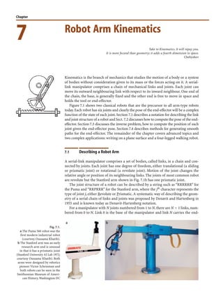
  • 1. 7 Chapter Kinematics is the branch of mechanics that studies the motion of a body or a system of bodies without consideration given to its mass or the forces acting on it. A serial- link manipulator comprises a chain of mechanical links and joints. Each joint can move its outward neighbouring link with respect to its inward neighbour. One end of the chain, the base, is generally fixed and the other end is free to move in space and holds the tool or end-effector. Figure 7.1 shows two classical robots that are the precursor to all arm-type robots today.Each robot has six joints and clearly the pose of the end-effector will be a complex function of the state of each joint.Section 7.1 describes a notation for describing the link and joint structure of a robot and Sect. 7.2 discusses how to compute the pose of the end- effector. Section 7.3 discusses the inverse problem, how to compute the position of each joint given the end-effector pose. Section 7.4 describes methods for generating smooth paths for the end-effector. The remainder of the chapter covers advanced topics and two complex applications: writing on a plane surface and a four-legged walking robot. 7.1 lDescribing a Robot Arm A serial-link manipulator comprises a set of bodies, called links, in a chain and con- nected by joints. Each joint has one degree of freedom, either translational (a sliding or prismatic joint) or rotational (a revolute joint). Motion of the joint changes the relative angle or position of its neighbouring links. The joints of most common robot are revolute but the Stanford arm shown in Fig. 7.1b has one prismatic joint. The joint structure of a robot can be described by a string such as “RRRRRR” for the Puma and “RRPRRR” for the Stanford arm, where the jth character represents the type of joint j, either Revolute or Prismatic. A systematic way of describing the geom- etry of a serial chain of links and joints was proposed by Denavit and Hartenberg in 1955 and is known today as Denavit-Hartenberg notation. For a manipulator with N joints numbered from 1 to N, there are N + 1 links, num- bered from 0 to N. Link 0 is the base of the manipulator and link N carries the end- Robot Arm Kinematics Take to Kinematics. It will repay you. It is more fecund than geometry; it adds a fourth dimension to space. Chebyshev Fig. 7.1. a The Puma 560 robot was the first modern industrial robot (courtesy Oussama Khatib). b The Stanford arm was an early research arm and is unusual in that it has a prismatic joint (Stanford University AI Lab 1972; courtesy Oussama Khatib). Both arms were designed by robotics pioneer Victor Scheinman and both robots can be seen in the Smithsonian Museum of Ameri- can History, Washington DC
  • 2. 138 effector or tool. Joint j connects link j − 1 to link j and therefore joint j moves link j.A link is considered a rigid body that defines the spatial relationship between two neighbouring joint axes.A link can be specified by two parameters,its length aj and its twist αj. Joints are also described by two parameters. The link offset dj is the distance from one link coordinate frame to the next along the axis of the joint.The joint angle θj is the rotation of one link with respect to the next about the joint axis. Figure 7.2 illustrates this notation.The coordinate frame {j} is attached to the far (dis- tal) end of link j.The axis of joint j is aligned with the z-axis.These link and joint param- eters are known as Denavit-Hartenberg parameters and are summarized in Table 7.1. Following this convention the first joint, joint 1, connects link 0 to link 1. Link 0 is the base of the robot. Commonly for the first link d1 = α1 = 0 but we could set d1 > 0 to represent the height of the shoulder joint above the base.In a manufacturing system the base is usually fixed to the environment but it could be mounted on a mobile base such as a space shuttle, an underwater robot or a truck. The final joint,joint Nconnects link N − 1 to link N.Link N is the tool of the robot and the parameters dN and aN specify the length of the tool and its x-axis offset respectively. The tool is generally considered to be pointed along the z-axis as shown in Fig. 2.14. The transformation from link coordinate frame {j − 1} to frame {j} is defined in terms of elementary rotations and translations as (7.1) which can be expanded as (7.2) Fig. 7.2. Definition of standard Denavit and Hartenberg link parameters. The colors red and blue denote all things associated with links j − 1 and j respectively. The numbers in circles represent the order in which the elementary trans- forms are applied Jacques Denavit and Richard Hartenberg introduced many of the key concepts of kinematics for serial-link manipulators in a 1955 paper (Denavit and Hartenberg 1955) and their later classic text Kinematic Synthesis of Linkages (Hartenberg and Denavit 1964). The 3 × 3 orthonormal matrix is aug- mented with a zero translational com- ponent to form a 4 × 4 homogenous transformation. Chapter 7 · Robot Arm Kinematics
  • 3. 139 The parameters αj and aj are always constant.For a revolute joint θj is the joint vari- able and dj is constant,while for a prismatic joint dj is variable,θj is constant and αj = 0. In many of the formulations that follow we use generalized joint coordinates For an N-axis robot the generalized joint coordinates q ∈ C where C ⊂ RN is called the joint space or configuration space. For the common case of an all-revolute robot C ⊂ SN the joint coordinates are referred to as joint angles. The joint coordinates are also referred to as the pose of the manipulator which is different to the pose of the end-effector which is a Cartesian pose ξ ∈ SE(3). The term configuration is shorthand for kinematic configuration which will be discussed in Sect. 7.3.1. Within the Toolbox we represent a robot link with a Link object which is created by >> L = Link([0, 0.1, 0.2, pi/2, 0]) L = theta=q, d=0.1, a=0.2, alpha=1.571 (R,stdDH) where the elements of the input vector are given in the order θk, dj, aj, αj. The optional fifth element σj indicates whether the joint is revolute (σi = 0) or prismatic (σi = 0). If not specified a revolute joint is assumed. The displayed values of the Link object shows its kinematic parameters as well as other status such the fact that it is a revolute joint (the tag R) and that the standard Denavit-Hartenberg parameter convention is used (the tag stdDH). Although a value was given for θ it is not displayed – that value simply served as a placeholder in the list of kinematic parameters.θ is substituted by the joint variable q and its value in the Link object is ignored. The value will be man- aged by the Link object. A Link object has many parameters and methods which are described in the online documentation, but the most common ones are illustrated by the following examples. The link transform Eq. 7.2 for q = 0.5 rad is Table 7.1. Denavit-Hartenberg parameters: their physical meaning, symbol and formal definition Jacques Denavit (1930–) was born in Paris where he studied for his Bachelor degree before pursuing his masters and doctoral degrees in mechanical engineering at Northwestern Univer- sity, Illinois. In 1958 he joined the Department of Mechanical Engineering and Astronautical Science at Northwestern where the collaboration with Hartenberg was formed. In addition to his interest in dynamics and kinematics Denavit was also interested in plasma physics and kinetics. After the publication of the book he moved to Lawrence Livermore National Lab, Livermore, California, where he undertook research on computer analysis of plasma physics problems. He retired in 1982. This is the same concept as was intro- duced for mobile robots on page 65. A slightly different notation, modifed Denavit-Hartenberg notation is dis- cussed in Sect. 7.5.3. 7.1 · Describing a Robot Arm
  • 4. 140 >> L.A(0.5) ans = 0.8776 -0.0000 0.4794 0.1755 0.4794 0.0000 -0.8776 0.0959 0 1.0000 0.0000 0.1000 0 0 0 1.0000 is a 4 × 4 homogeneous transformation. Various link parameters can be read or al- tered, for example >> L.RP ans = R indicates that the link is prismatic and >> L.a ans = 0.2000 returns the kinematic parameter a. Finally a link can contain an offset >> L.offset = 0.5; >> L.A(0) ans = 0.8776 -0.0000 0.4794 0.1755 0.4794 0.0000 -0.8776 0.0959 0 1.0000 0.0000 0.1000 0 0 0 1.0000 which is added to the joint variable before computing the link transform and will be discussed in more detail in Sect. 7.5.1. 7.2 lForward Kinematics The forward kinematics is often expressed in functional form (7.3) with the end-effector pose as a functionof joint coordinates.Using homogeneoustrans- formations this is simply the product of the individual link transformation matrices given by Eq. 7.2 which for an N-axis manipulator is (7.4) The forward kinematic solution can be computed for any serial-link manipulator irrespective of the number of joints or the types of joints. Determining the Denavit- Hartenberg parameters for each of the robot’s links is described in more detail in Sect. 7.5.2. The pose of the end-effector ξE ∼ TE ∈ SE(3) has six degrees of freedom – three in translation and three in rotation. Therefore robot manipulators commonly have six joints or degrees of freedom to allow them to achieve an arbitrary end-effector pose. The overall manipulator transform is frequently written as T6 for a 6-axis robot. Richard Hartenberg (1907–1997) was born in Chicago and studied for his degrees at the University of Wisconsin,Madison.He served in the merchant marine and studied aeronautics for two years at the University of Goettingen with space-flight pioneer Theodor von Karman.He was Professor of mechanical engineering at Northwestern University where he taught for 56 years. His research in kinematics led to a revival of interest in this field in the 1960s,and his efforts helped put kinemat- ics on a scientific basis for use in computer applications in the analysis and design of complex mechanisms. His also wrote extensively on the history of mechanical engineering. Chapter 7 · Robot Arm Kinematics
  • 5. 141 7.2.1 lA 2-Link Robot The first robot that we will discuss is the two-link planar manipulator shown in Fig. 7.3. It has the following Denavit-Hartenberg parameters which we use to create a vector of Link objects Fig. 7.3. Two-link robot as per Spong et al. (2006, fig. 3.6, p. 84) >> L(1) = Link([0 0 1 0]); >> L(2) = Link([0 0 1 0]); >> L L = theta=q1, d=0, a=1, alpha=0 (R,stdDH) theta=q2, d=0, a=1, alpha=0 (R,stdDH) which are passed to the constructor SerialLink >> two_link = SerialLink(L, 'name', 'two link'); which returns a SerialLink object that we can display >> two_link two_link = two link (2 axis, RR, stdDH) +---+-----------+-----------+-----------+-----------+ | j | theta | d | a | alpha | +---+-----------+-----------+-----------+-----------+ | 1| q1| 0| 1| 0| | 2| q2| 0| 1| 0| +---+-----------+-----------+-----------+-----------+ grav = 0 base = 1 0 0 0 tool = 1 0 0 0 0 0 1 0 0 0 1 0 0 9.81 0 0 1 0 0 0 1 0 0 0 0 1 0 0 0 1 7.2 · Forward Kinematics
  • 6. 142 This provides a concise description of the robot. We see that it has 2 revolute joints as indicated by the structure string 'RR', it is defined in terms of standard Denavit- Hartenberg parameters, that gravity is acting in the default z-direction. The kine- matic parameters of the link objects are also listed and the joint variables are shown as variables q1 and q2. We have also assigned a name to the robot which will be shown whenever the robot is displayed graphically. The script >> mdl_twolink performs the above steps and defines this robot in the MATLAB® workspace, creating a SerialLink object named twolink. The SerialLink object is key to the operation of the Robotics Toolbox. It has a great many methods and properties which are illustrated in the rest of this part, and described in detail in the online documentation. Some simple examples are >> twolink.n ans = 2 which returns the number of joints, and >> links = twolink.links L = theta=q1, d=0, a=1, alpha=0 (R,stdDH) theta=q2, d=0, a=1, alpha=0 (R,stdDH) which returns a vector of Link objects comprising the robot. We can also make a copy of a SerialLink object >> clone = SerialLink(twolink, 'name', 'bob') clone = bob (2 axis, RR, stdDH) +---+-----------+-----------+-----------+-----------+ | j | theta | d | a | alpha | +---+-----------+-----------+-----------+-----------+ | 1| q1| 0| 1| 0| | 2| q2| 0| 1| 0| +---+-----------+-----------+-----------+-----------+ grav = 0 base = 1 0 0 0 tool = 1 0 0 0 0 0 1 0 0 0 1 0 0 9.81 0 0 1 0 0 0 1 0 0 0 0 1 0 0 0 1 which has the name 'bob'. Now we can put the robot arm to work. The forward kinematics are computed us- ing the fkine method. For the case where q1 = q2 = 0 >> twolink.fkine([0 0]) ans = 1 0 0 2 0 1 0 0 0 0 1 0 0 0 0 1 the method returns the homogenous transform that represents the pose of the second link coordinate frame of the robot, T2. For a different configuration the tool pose is >> twolink.fkine([pi/4 -pi/4]) ans = 1.0000 0 0 1.7071 0 1.0000 0 0.7071 0 0 1.0000 0 0 0 0 1.0000 By convention, joint coordinates with the Toolbox are row vectors. Normal to the plane in which the robot moves. Link objects are derived from the MATLAB® handle class and can be set in place.Thus we can write code like twolink.links(1).a = 2 to change the kinematic parameter a2. A unique name is required when mul- tiple robots are displayed graphically, see Sect. 7.8 for more details. Chapter 7 · Robot Arm Kinematics
  • 7. 143 The robot can be visualized graphically >> twolink.plot([0 0]) >> twolink.plot([pi/4 -pi/4]) as stick figures shown in Fig. 7.4. The graphical representation includes the robot’s name, the final-link coordinate frame, T2 in this case, the joints and their axes, and a shadow on the ground plane. Additional features of the plot method such as mul- tiple views and multiple robots are described in Sect. 7.8 with additional details in the online documentation. The simple two-link robot introduced above is limited in the poses that it can achieve since it operates entirely within the xy-plane, its task space is T ⊂ R2. 7.2.2 lA 6-Axis Robot Truly useful robots have a task space T ⊂ SE(3) enabling arbitrary position and atti- tude of the end-effector – the task space has six spatial degrees of freedom: three trans- lational and three rotational. This requires a robot with a configuration space C ⊂ R6 which can be achieved by a robot with six joints.In this section we will use the Puma 560 as an example of the class of all-revolute six-axis robot manipulators. We define an instance of a Puma 560 robot using the script >> mdl_puma560 which creates a SerialLink object, p560, in the workspace >> p560 p560 = Puma 560 (6 axis, RRRRRR, stdDH) Unimation; viscous friction; params of 8/95; +---+-----------+-----------+-----------+-----------+ | j | theta | d | a | alpha | +---+-----------+-----------+-----------+-----------+ | 1| q1| 0| 0| 1.571| | 2| q2| 0| 0.4318| 0| | 3| q3| 0.15| 0.0203| -1.571| | 4| q4| 0.4318| 0| 1.571| | 5| q5| 0| 0| -1.571| | 6| q6| 0| 0| 0| +---+-----------+-----------+-----------+-----------+ grav = 0 base = 1 0 0 0 tool = 1 0 0 0 0 0 1 0 0 0 1 0 0 9.81 0 0 1 0 0 0 1 0 0 0 0 1 0 0 0 1 Fig. 7.4. Thetwo-linkrobotintwo different poses, a the pose (0, 0); b the pose (ý , −ý). Note the graphical details. Revolute joints are indicated by cylinders and the joint axes are shown as line seg- ments. The final-link coordinate frameandashadowontheground are also shown TheToolbox has scripts to define a num- ber of common industrial robots in- cluding the Motoman HP6, Fanuc 10L, ABB S4 2.8 and the Stanford arm. 7.2 · Forward Kinematics
  • 8. 144 Note that aj and dj are in SI units which means that the translational part of the for- ward kinematics will also have SI units. The script mdl_puma560 also creates a number of joint coordinate vectors in the workspace which represent the robot in some canonic configurations: qz (0, 0, 0, 0, 0, 0) zero angle qr (0, ü, −ü , 0, 0, 0) ready, the arm is straight and vertical qs (0, 0, −ü , 0, 0, 0) stretch, the arm is straight and horizontal qn (0, ý , −π, 0, ý, 0) nominal, the arm is in a dextrous working pose and these are shown graphically in Fig. 7.5. These plots are generated using the plot method, for example >> p560.plot(qz) The Puma 560 robot (Programmable Universal Manipulator for Assembly) shown in Fig. 7.1 was released in 1978 and became enormously popular. It featured an anthropomorphic design, elec- tric motors and a spherical wrist which makes it the first modern industrial robot – the archetype of all that followed. The Puma 560 catalyzed robotics research in the 1980s and it was a very common laboratory robot. Today it is obsolete and rare but in homage to its important role in robotics research we use it here. For our purposes the advantages of this robot are that it has been well studied and its parameters are very well known – it has been described as the “white rat” of robotics research. Most modern 6-axis industrial robots are very similar in structure and can be accomodated simply by changing the Denavit-Hartenberg parameters. The Toolbox has kinematic models for a number of common industrial robots including the Motoman HP6, Fanuc 10L, and ABB S4 2.8. Fig. 7.5. The Puma robot in 4 dif- ferent poses.a Zero angle;b ready pose; c stretch; d nominal Well awayfrom singularities,which will be discussed in Sect. 7.4.3. Chapter 7 · Robot Arm Kinematics
  • 9. 145 Forward kinematics can be computed as before >> p560.fkine(qz) ans = 1.0000 0 0 0.4521 0 1.0000 0 -0.1500 0 0 1.0000 0.4318 0 0 0 1.0000 which returns the homogeneous transformation corresponding to the end-effector pose T6. The origin of this frame, the link 6 coordinate frame {6}, is defined as the point of intersection of the axes of the last 3 joints – physically this point is inside the robot’s wrist mechanism. We can define a tool transform, from the T6 frame to the actual tool tip by >> p560.tool = transl(0, 0, 0.2); in this case a 200 mm extension in the T6 z-direction. The pose of the tool tip, often referred to as the tool centre point or TCP, is now >> p560.fkine(qz) ans = 1.0000 0 0 0.4521 0 1.0000 0 -0.1500 0 0 1.0000 0.6318 0 0 0 1.0000 The kinematic definition we have used considers that the base of the robot is the inter- section point of the waist and shoulder axes which is a point inside the structure of the robot. The Puma 560 robot includes a 30 inch tall pedestal.We can shift the origin of the robot from the point inside the robot to the base of the pedestal using a base transform >> p560.base = transl(0, 0, 30*0.0254); where for consistency we have converted the pedestal height to SI units. Now, with both base and tool transform, the forward kinematics are >> p560.fkine(qz) ans = 1.0000 0 0 0.4521 0 1.0000 0 -0.1500 0 0 1.0000 1.3938 0 0 0 1.0000 and we can see that the z-coordinate of the tool is now greater than before. We can also do more interesting things, for example >> p560.base = transl(0,0,3) * trotx(pi); >> p560.fkine(qz) ans = 1.0000 0 0 0.4521 0 -1.0000 -0.0000 0.1500 0 0.0000 -1.0000 2.3682 0 0 0 1.0000 which positions the robot’s origin 3 m above the world origin with its coordinate frame rotated by 180° about the x-axis. This robot is now hanging from the ceiling! Anthropomorphic means having human-like characteristics. The Puma 560 robot was designed to have approximately the dimensions and reach of a human worker. It also had a spherical joint at the wrist just as humans have. Roboticists also tend to use anthropomorphic terms when describing robots. We use words like waist, shoulder, elbow and wrist when describing serial link manipulators. For the Puma these terms correspond respectively to joint 1, 2, 3 and 4–6. By the mdl_puma560 script. Alternatively we could change the ki- nematic parameter d6. The tool trans- form approach is more general since thefinallinkkinematicparametersonly allow setting of d6, a6 and α6 which provide z-axis translation, x-axis trans- lation and x-axis rotation respectively. 7.2 · Forward Kinematics
  • 10. 146 The Toolbox supports joint angle time series or trajectories such as >> q q = 0 0 0 0 0 0 0 0.0365 -0.0365 0 0 0 0 0.2273 -0.2273 0 0 0 0 0.5779 -0.5779 0 0 0 0 0.9929 -0.9929 0 0 0 0 1.3435 -1.3435 0 0 0 0 1.5343 -1.5343 0 0 0 0 1.5708 -1.5708 0 0 0 where each row represents the joint coordinates at a different timestep and the col- umns represent the joints. In this case the method fkine >> T = p560.fkine(q); returns a 3-dimensional matrix >> about(T) T [double] : 4x4x8 (1024 bytes) where the first two dimensions are a 4 × 4 homogeneous transformation and the third dimension is the timestep. The homogeneous transform corresponding to the joint coordinates in the fourth row of q is >> T(:,:,4) ans = 1.0000 0.0000 0 0.3820 0.0000 1.0000 -0.0000 -0.1500 0 -0.0000 1.0000 1.6297 0 0 0 1.0000 Creating a trajectory is the topic of Sect. 7.4. 7.3 lInverse Kinematics We have shown how to determine the pose of the end-effector given the joint coordi- nates and optional tool and base transforms.A problem of real practical interest is the inverse problem: given the desired pose of the end-effector ξE what are the required joint coordinates? For example, if we know the Cartesian pose of an object, what joint coordinates does the robot need in order to reach it? This is the inverse kinematics problem which is written in functional form as (7.5) Ingeneral this function is not unique and for some classes of manipulator no closed- form solution exists, necessitating a numerical solution. 7.3.1 lClosed-Form Solution A necessary condition for a closed-form solution of a 6-axis robot is that the three wrist axes intersect at a single point. This means that motion of the wrist joints only changes the end-effector orientation, not its translation. Such a mechanism is known as a spherical wrist and almost all industrial robots have such wrists. We will explore inverse kinematics using the Puma robot model >> mdl_puma560 Generated by the jtraj function, which is discussed in Sect. 7.4.1. Chapter 7 · Robot Arm Kinematics
  • 11. 147 At the nominal joint coordinates >> qn qn = 0 0.7854 3.1416 0 0.7854 0 the end-effector pose is >> T = p560.fkine(qn) T = -0.0000 0.0000 1.0000 0.5963 -0.0000 1.0000 -0.0000 -0.1501 -1.0000 -0.0000 -0.0000 -0.0144 0 0 0 1.0000 Since the Puma 560 is a 6-axis robot arm with a spherical wrist we use the method ikine6s to compute the inverse kinematics using a closed-form solution. The re- quired joint coordinates to achieve the pose T are >> qi = p560.ikine6s(T) qi = 2.6486 -3.9270 0.0940 2.5326 0.9743 0.3734 Surprisingly, these are quite different to the joint coordinates we started with. How- ever if we investigate a little further >> p560.fkine(qi) ans = -0.0000 0.0000 1.0000 0.5963 0.0000 1.0000 -0.0000 -0.1500 -1.0000 0.0000 -0.0000 -0.0144 0 0 0 1.0000 we see that these two different sets of joint coordinates result in the same end-effector pose and these are shown in Fig. 7.6. The shoulder of the Puma robot is horizontally offset from the waist, so in one solution the arm is to the left of the waist, in the other it is to the right. These are referred to as the left- and right-handed kinematic con- figurations respectively. In general there are eight sets of joint coordinates that give the same end-effector pose – as mentioned earlier the inverse solution is not unique. We can force the right-handed solution >> qi = p560.ikine6s(T, 'ru') qi = -0.0000 0.7854 3.1416 0.0000 0.7854 -0.0000 which gives the original set of joint angles by specifying a right handed configuration with the elbow up. In addition to the left- and right-handed solutions, there are solutions with the elbow either up or down, and with the wrist flipped or not flipped. For the Puma 560 robot the wrist joint, θ4, has a large rotational range and can adopt one of two angles Fig. 7.6. Two solutions to the in- verse kinematic problem, left- handed and right-handed solu- tions. The shadow shows clearly the two different configurations Themethodikine6scheckstheDe- navit-Hartenberg parameters to deter- mine if the robot meets these criteria. Morepreciselytheelbowisaboveorbe- low the shoulder. 7.3 · Inverse Kinematics
  • 12. 148 that differ by π rad. Since most robot grippers have just two fingers, see Fig. 2.14, this makes no difference in its ability to grasp an object. The various kinematic configurations are shown in Fig. 7.7. The kinematic con- figuration returned by ikine6s is controlled by one or more of the character flags: left or right handed 'l', 'r' elbow up or down 'u', 'd' wrist flipped or not flipped 'f', 'n' Due to mechanical limits on joint angles and possible collisions between links not all eight solutions are physically achievable. It is also possible that no solution can be achieved, for example >> p560.ikine6s( transl(3, 0, 0) ) Warning: point not reachable ans = NaN NaN NaN NaN NaN NaN fails because the arm is simply not long enough to reach this pose.A pose may also be unachievable due to singularity where the alignment of axes reduces the effective de- grees of freedom (the gimbal lock problem again). The Puma 560 has a singularity when q5 is equal to zero and the axes of joints 4 and 6 become aligned. In this case the best that ikine6s can do is to constrain q4 + q6 but their individual values are arbi- trary. For example consider the configuration >> q = [0 pi/4 pi 0.1 0 0.2]; for which q4 + q6 = 0.3. The inverse kinematic solution is >> p560.ikine6s(p560.fkine(q), 'ru') ans = -0.0000 0.7854 3.1416 2.9956 0.0000 -2.6956 Fig. 7.7. Different configurations of the Puma 560 robot. a Right- up-noflip; b right-down-noflip; c right-down-flip Chapter 7 · Robot Arm Kinematics
  • 13. 149 has quite different values for q4 and q6 but their sum >> q(4)+q(6) ans = 0.3000 remains the same. 7.3.2 lNumerical Solution For the case of robots which do not have six joints and a spherical wrist we need to use an iterative numerical solution. Continuing with the example of the previous section we use the method ikine to compute the general inverse kinematic solution >> T = p560.fkine(qn) ans = -0.0000 0.0000 1.0000 0.5963 -0.0000 1.0000 -0.0000 -0.1501 -1.0000 -0.0000 -0.0000 -0.0144 0 0 0 1.0000 >> qi = p560.ikine(T) qi = 0.0000 -0.8335 0.0940 -0.0000 -0.8312 0.0000 which is different to the original value >> qn qn = 0 0.7854 3.1416 0 0.7854 0 but does result in the correct tool pose >> p560.fkine(qi) ans = -0.0000 0.0000 1.0000 0.5963 -0.0000 1.0000 -0.0000 -0.1501 -1.0000 -0.0000 -0.0000 -0.0144 0 0 0 1.0000 Plotting the pose >> p560.plot(qi) shows clearly that ikine has found the elbow-down configuration. A limitation of this general numeric approach is that it does not provide explicit control over the arm’s kinematic configuration as did the analytic approach – the only control is implicit via the initial value of joint coordinates (which defaults to zero). If we specify the initial joint coordinates >> qi = p560.ikine(T, [0 0 3 0 0 0]) qi = 0.0000 0.7854 3.1416 0.0000 0.7854 -0.0000 the solution converges on the elbow-up configuration. Aswouldbeexpectedthegeneralnumericalapproachof ikineisconsiderablyslower than the analytic approach of ikine6s. However it has the great advantage of being able to work with manipulators at singularities and manipulators with less than six or more than six joints. Details of the principle behind ikine is provided in Sect. 8.4. 7.3.3 lUnder-Actuated Manipulator An under-actuated manipulator is one that has fewer than six joints, and is therefore limitedintheend-effectorposesthatitcanattain.SCARArobotssuchasshownonpage 135 are a common example, they have typically have an x-y-z-θ task space, T ⊂ R3 × S and a configuration space C ⊂ S3 × R. 7.3 · Inverse Kinematics Whensolvingforatrajectoryasonp.146 the inverse kinematic solution for one point is used to initialize the solution for the next point on the path.
  • 14. 150 We will revisit the two-link manipulator example from Sect. 7.2.1,first defining the robot >> mdl_twolink and then defining the desired end-effector pose >> T = transl(0.4, 0.5, 0.6); However this pose is over-constrained for the two-link robot – the tool cannot meet the orientation constraint on the direction of '2 and (2 nor a z-axis translational value other than zero. Therefore we require the ikine method to consider only er- ror in the x- and y-axis translational directions, and ignore all other Cartesian de- grees of freedom.We achieve this by specifying a mask vector as the fourth argument >> q = twolink.ikine(T, [0 0], [1 1 0 0 0 0]) q = -0.3488 2.4898 The elements of the mask vector correspond respectively to the three translations and three orientations: tx, ty, tz, rx, ry, rz in the end-effector coordinate frame. In this example we specified that only errors in x- and y-translation are to be considered (the non-zero elements). The resulting joint angles correspond to an endpoint pose >> twolink.fkine(q) ans = ans = -0.5398 -0.8418 0 0.4000 0.8418 -0.5398 0 0.5000 0 0 1.0000 0 0 0 0 1.0000 which has the desired x- and y-translation, but the orientation and z-translation are incorrect, as we allowed them to be. 7.3.4 lRedundant Manipulator A redundant manipulator is a robot with more than six joints. As mentioned previ- ously, six joints is theoretically sufficient to achieve any desired pose in a Cartesian taskspace T ⊂ SE(3). However practical issues such as joint limits and singularities mean that not all poses within the robot’s reachable space can be achieved. Adding additional joints is one way to overcome this problem. To illustrate this we will create a redundant manipulator. We place our familiar Puma robot >> mdl_puma560 onaplatformthatmovesinthexy-plane,mimickingarobotmountedonavehicle.Thisrobot hasthesametaskspaceT ⊂ SE(3)asthePumarobot,butaconfigurationspaceC ⊂ R2 × S6. The dimension of the configuration space exceeds the dimensions of the task space. The Denavit-Hartenberg parameters for the base are and using a shorthand syntax we create the SerialLink object directly from the Denavit-Hartenberg parameters >> platform = SerialLink( [0 0 0 -pi/2 1; -pi/2 0 0 pi/2 1], ... 'base', troty(pi/2), 'name', 'platform' ); Chapter 7 · Robot Arm Kinematics
  • 15. 151 The Denavit-Hartenberg notation requires that prismatic joints cause translation in the local z-direction and the base-transform rotates that z-axis into the world x-axis direction. This is a common complexity with Denavit-Hartenberg notation and an alternative will be introduced in Sect. 7.5.2. The joint coordinates of this robot are its x- and y-position and we test that our Denavit-Hartenberg parameters are correct >> platform.fkine([1, 2]) ans = 1.0000 0.0000 0.0000 1.0000 -0.0000 1.0000 0.0000 2.0000 0 -0.0000 1.0000 0.0000 0 0 0 1.0000 We see that the rotation submatrix is the identity matrix, meaning that the coordinate frame of the platform is parallel with the world coordinate frame, and that the x- and y-displacement is as requested. We mount the Puma robot on the platform by connecting the two robots in series. In the Toolbox we can express this in two different ways, by multiplication >> p8 = platform * p560; or by concatenation p8 = SerialLink( [platform, p560]); which also allows other attributes of the created SerialLink object to be specified. However there is a small complication.We would like the Puma arm to be sitting on its tall pedestal on top of the platform. Previously we added the pedestal as a base transform, but base transforms can only exist at the start of a kinematic chain, and we require the transform between joints 2 and 3 of the 8-axis robot.Instead we implement the pedestal by setting d1 of the Puma to the pedestal height >> p560.links(1).d = 30 * 0.0254; and now we can compound the two robots >> p8 = SerialLink( [platform, p560], 'name', 'P8') p8 = P8 (8 axis, PPRRRRRR, stdDH) +---+-----------+-----------+-----------+-----------+ | j | theta | d | a | alpha | +---+-----------+-----------+-----------+-----------+ | 1| 0| q1| 0| -1.571| | 2| -1.571| q2| 0| 1.571| | 3| q3| 0.762| 0| 1.571| | 4| q4| 0| 0.4318| 0| | 5| q5| 0.15| 0.0203| -1.571| | 6| q6| 0.4318| 0| 1.571| | 7| q7| 0| 0| -1.571| | 8| q8| 0| 0| 0| +---+-----------+-----------+-----------+-----------+ grav = 0 base = 0 0 0 0 tool = 1 0 0 0 0 0 1 0 0 0 1 0 0 9.81 1 0 0 0 0 0 1 0 0 0 0 1 0 0 0 1 resulting in a new 8-axis robot which we have named the P8. We note that the new robot has inherited the base transform of the platform, and that the pedestal displace- ment appears now as d3. We can find the inverse kinematics for this new redundant manipulator using the general numerical solution.For example to move the end effector to (0.5, 1.0, 0.7) with the tool pointing downward in the xz-plane the Cartesian pose is 7.3 · Inverse Kinematics
  • 16. 152 >> T = transl(0.5, 1.0, 0.7) * rpy2tr(0, 3*pi/4, 0); The required joint coordinates are >> qi = p8.ikine(T) qi = -0.3032 1.0168 0.1669 -0.4908 -0.6995 -0.1276 -1.1758 0.1679 The first two elements are displacements of the prismatic joints in the base, and the last six are the robot arm’s joint angles.We see that the solution has made good use of the second joint, the platform’s y-axis translation to move the base of the arm close to the desired point. We can visualize the configuration >> p8.plot(qi) which is shown in Fig. 7.8.We can also show that the plain old Puma cannot reach the point we specified >> p560.ikine6s(T) Warning: point not reachable This robot has 8 degrees of freedom. Intuitively it is more dextrous than its 6-axis counterpart because there is more than one joint that can contribute to every Carte- sian degree of freedom. This is more formally captured in the notion of manipulabil- ity which we will discuss in Sect. 8.1.4. For now we will consider it as a scalar measure that reflects the ease with which the manipulator’s tool can move in different Carte- sian directions. The manipulability of the 6-axis robot >> p560.maniplty(qn) ans = 0.0786 is much less than that for the 8-axis robot >> p8.maniplty([0 0 qn]) ans = 1.1151 which indicates the increased dexterity of the 8-axis robot. 7.4 lTrajectories One of the most common requirements in robotics is to move the end-effector smoothly from pose A to pose B. Building on what we learnt in Sect. 3.1 we will discuss two ap- proaches to generating such trajectories: straight lines in joint space and straight lines in Cartesian space. These are known respectively as joint-space and Cartesian motion. Fig. 7.8. Redundant manipulator P8 Chapter 7 · Robot Arm Kinematics
  • 17. 153 7.4.1 lJoint-Space Motion Consider the end-effector moving between two Cartesian poses >> T1 = transl(0.4, 0.2, 0) * trotx(pi); >> T2 = transl(0.4, -0.2, 0) * trotx(pi/2); which lie in the xy-plane with the end-effector oriented downward. The initial and final joint coordinate vectors associated with these poses are >> q1 = p560.ikine6s(T1); >> q2 = p560.ikine6s(T2); and we require the motion to occur over a time period of 2 seconds in 50 ms time steps >> t = [0:0.05:2]'; A joint-space trajectory is formed by smoothly interpolating between two configurations q1 and q2. The scalar interpolation functions tpoly or lspb from Sect. 3.1 can be used in conjunction with the multi-axis driver function mtraj >> q = mtraj(@tpoly, q1, q2, t); or >> q = mtraj(@lspb, q1, q2, t); which each result in a 50 × 6 matrix q with one row per time step and one column per joint. From here on we will use the jtraj convenience function >> q = jtraj(q1, q2, t); which is equivalent to mtraj with tpoly interpolation but optimized for the multi- axis case and also allowing initial and final velocity to be set using additional argu- ments. For mtraj and jtraj the final argument can be a time vector, as here, or an integer specifying the number of time steps. We obtain the joint velocity and acceleration vectors, as a function of time,through optional output arguments >> [q,qd,qdd] = jtraj(q1, q2, t); An even more concise expression for the above steps is provided by the jtraj method of the SerialLink class >> q = p560.jtraj(T1, T2, t) The trajectory is best viewed as an animation >> p560.plot(q) but we can also plot the joint angle, for instance q2, versus time >> plot(t, q(:,2)) or all the angles versus time >> qplot(t, q); as shown in Fig. 7.9a. The joint coordinate trajectory is smooth but we do not know how the robot’s end-effector will move in Cartesian space. However we can easily determine this by applying forward kinematics to the joint coordinate tra- jectory >> T = p560.fkine(q); Wechoosethetoolz-axisdownwardon these poses as it would be if the robot was reaching down to work on some horizontalsurface.ForthePuma 560ro- bot it be physically impossible for the tool z-axis to point upward in such a situation. 7.4 · Trajectories
  • 18. 154 which results in a 3-dimensional Cartesian trajectory. The translational part of this trajectory is >> p = transl(T); which is in matrix form >> about(p) p [double] : 41x3 (984 bytes) and has one row per time step,and each row is the end-effector position vector.This is plotted against time in Fig. 7.9b. The path of the end-effector in the xy-plane >> plot(p(:,1), p(:,2)) is shown in Fig. 7.9c and it is clear that the path is not a straight line. This is to be expected since we only specified the Cartesian coordinates of the end-points. As the robot rotates about its waist joint during the motion the end-effector will naturally follow a circular arc. In practice this could lead to collisions between the robot and nearby objects even if they do not lie on the path between poses A and B. The orienta- tion of the end-effector, in roll-pitch-yaw angles form, can be plotted against time >> plot(t, tr2rpy(T)) as shown in Fig. 7.9d. Note that the roll angle varies from π to ü as we specified. However while the pitch angle has met its boundary conditions it has varied along Fig. 7.9. Jointspacemotion.a Joint coordinates versus time; b Carte- sian position versus time; c Carte- sian position locus in the xy-plane d roll-pitch-yawanglesversustime Rotation about x-axis from Sect. 2.2.1.2. Chapter 7 · Robot Arm Kinematics
  • 19. 155 the path.Also note that the initial roll angle is shown as −π but at the next time step it is π.This is an artifact of finite precision arithmetic and both angles are equivalent on the circle. We can also implement this example in Simulink® >> sl_jspace and the block diagram model is shown in Fig. 7.10. The parameters of the jtraj block are the initial and final values for the joint coordinates and the time duration of the motion segment. The smoothly varying joint angles are wired to a plot block which will animate a robot in a separate window, and to an fkine block to compute the forward kinematics. Both the plot and fkine blocks have a parameter which is a SerialLink object, in this case p560. The Cartesian position of the end-effector pose is extracted using the T2xyz block which is analogous to the Toolbox function transl. The XY Graph block plots y against x. 7.4.2 lCartesian Motion For many applications we require straight-line motion in Cartesian space which is known as Cartesian motion. This is implemented using the Toolbox function ctraj which was introduced in Chap. 3. Its usage is very similar to jtraj >> Ts = ctraj(T1, T2, length(t)); where the arguments are the initial and final pose and the number of time steps and it returns the trajectory as a 3-dimensional matrix. As for the previous joint-space example we will extract and plot the translation >> plot(t, transl(Ts)); and orientation components >> plot(t, tr2rpy(Ts)); of this motion which is shown in Fig. 7.11 along with the path of the end-effector in the xy-plane. Compared to Fig. 7.9b and c we note some important differences. Firstly the position and orientation, Fig. 7.11b and d vary linearly with time. For orientation the pitch angle is constant at zero and does not vary along the path. Secondly the end- effector follows a straight line in the xy-plane as shown in Fig. 7.9c. The corresponding joint-space trajectory is obtained by applying the inverse ki- nematics >> qc = p560.ikine6s(Ts); and is shown in Fig. 7.11a.While broadly similar to Fig. 7.9a the minor differences are what result in the straight line Cartesian motion. Fig. 7.10. Simulink® model sl_jspace for joint-space motion The Simulink® integration time needs to besetequaltothemotionsegmenttime, through the Simulation menu or from the MATLAB® command line >> sim('sl_jspace', 10);. 7.4 · Trajectories
  • 20. 156 7.4.3 lMotion through a Singularity We have already briefly touched on the topic of singularities (page 148) and we will revisit it again in the next chapter.In the next example we deliberately choose a trajec- tory that moves through a robot singularity.We change the Cartesian endpoints of the previous example to >> T1 = transl(0.5, 0.3, 0.44) * troty(pi/2); >> T2 = transl(0.5, -0.3, 0.44) * troty(pi/2); which results in motion in the y-direction with the end-effector z-axis pointing in the x-direction. The Cartesian path is >> Ts = ctraj(T1, T2, length(t)); which we convert to joint coordinates >> qc = p560.ikine6s(Ts) and is shown in Fig. 7.12a. At time t ≈ 0.7 s we observe that the rate of change of the wrist joint angles q4 and q6 has become very high. The cause is that q5 has become almost zero which means that the q4 and q6 rotational axes are almost aligned – an- other gimbal lock situation or singularity. Fig. 7.11. Cartesianmotion.aJoint coordinates versus time; b Carte- sian position versus time; c Carte- sianpositionlocusinthexy-plane; d roll-pitch-yawanglesversustime q6 has increased rapidly, while q4 has decreased rapidly and wrapped around from −π to π. Chapter 7 · Robot Arm Kinematics
  • 21. 157 The joint alignment means that the robot has lost one degree of freedom and is now effectively a 5-axis robot.Kinematically we can only solve for the sum q4 + q6 and there are an infinite number of solutions for q4 and q6 that would have the same sum. The joint-space motion between the two poses, Fig. 7.12b, is immune to this problem since it is does not require the inverse kinematics. However it will not maintain the pose of the tool in the x-direction for the whole path – only at the two end points. From Fig. 7.12c we observe that the generalized inverse kinematics method ikine handles the singularity with ease. The manipulability measure for this path >> m = p560.maniplty(qc); is plotted in Fig. 7.12d and shows that manipulability was almost zero around the time of the rapid wrist joint motion.Manipulability and the generalized inverse kinematics func- tion are based on the manipulator’s Jacobian matrix which is the topic of the next chapter. 7.4.4 lConfiguration Change Earlier (page 147) we discussed the kinematic configuration of the manipulator arm and how it can work in a left- or right-handed manner and with the elbow up or down. Consider the problem of a robot that is working for a while left-handed at one work Fig.7.12.Cartesianmotionthrough a wrist singularity. a Joint coordi- nates computed by inverse kine- matics(ikine6s);b jointcoordi- nates computed by generalized in- verse kinematics (ikine); c joint coordinatesforjoint-spacemotion; d manipulability 7.4 · Trajectories
  • 22. 158 station, then working right-handed at another. Movement from one configuration to another ultimately results in no change in the end-effector pose since both configura- tion have the same kinematic solution – therefore we cannot create a trajectory in Cartesian space. Instead we must use joint-space motion. For example to move the robot arm from the right- to left-handed configuration we first define some end-effector pose >> T = transl(0.4, 0.2, 0) * trotx(pi); and then determine the joint coordinates for the right- and left-handed elbow-up con- figurations >> qr = p560.ikine6s(T, 'ru'); >> ql = p560.ikine6s(T, 'lu'); and then create a path between these two joint coordinates >> q = jtraj(qr, ql, t); Although the initial and final end-effector pose is the same, the robot makes some quite significant joint space motion as shown in Fig. 7.13 – in the real world you need to be careful the robot doesn’t hit something.Once again, the best way to visualize this is in animation >> p560.plot(q) 7.5 lAdvanced Topics 7.5.1 lJoint Angle Offsets The pose of the robot with zero joint angles is frequently some rather unusual (or even mechanically unachievable) pose. For the Puma robot the zero-angle pose is a non-obvious L-shape with the upper arm horizontal and the lower arm vertically upward as shown in Fig. 7.5a. This is a consequence of constraints imposed by the Denavit-Hartenberg formalism. A robot control designer may choose the zero-angle configuration to be something more obvious such as that shown in Fig. 7.5b or c. The joint coordinate offset provides a mechanism to set an arbitrary configu- ration for the zero joint coordinate case. The offset vector, q0, is added to the user specified joint angles before any kinematic or dynamic function is invoked, for example Fig. 7.13. Joint space motions for con- figuration change from right- handed to left-handed It is actually implemented within the Link object. Chapter 7 · Robot Arm Kinematics
  • 23. 159 (7.6) Similarly it is subtracted after an operation such as inverse kinematics (7.7) The offset is set by assigning the offset property of the Link object, for example >> L = Link([0 0 1 0]); >> L.offset = pi/4 or >> p560.links(2).offset = pi/2; 7.5.2 lDetermining Denavit-Hartenberg Parameters The classical method of determining Denavit-Hartenberg parameters is to systemati- cally assign a coordinate frame to each link.The link frames for the Puma robot using the standardDenavit-HartenbergformalismareshowninFig. 7.14a.Howevertherearestrong constraints on placing each frame since joint rotation must be about the z-axis and the link displacement must be in the x-direction. This in turn imposes constraints on the placement of the coordinate frames for the base and the end-effector,and ultimately dic- tates the zero-angle pose just discussed. Determining the Denavit-Hartenberg param- eters and link coordinate frames for a completely new mechanism is therefore more dif- ficult than it should be – even for an experienced roboticist. Fig. 7.14. Puma 560 robot coordinate frames. a Standard Denavit-Har- tenberg link coordinate frames for Puma in the zeroangle pose (Corke 1996b); b alternative approach showing the sequence of elemen- tary transforms from base to tip. Rotations are about the axes shown as dashed lines (Corke 2007) 7.5 · Advanced Topics
  • 24. 160 An alternative approach, supported by the Toolbox, is to simply describe the ma- nipulator as a series of elementary translations and rotations from the base to the tip of the end-effector.Some of the the elementary operations are constants such as trans- lations that represent link lengths or offsets,and some are functions of the generalized joint coordinates qi. Unlike the conventional approach we impose no constraints on the axes about which these rotations or translations can occur. An example for the Puma robot is shown in Fig. 7.14b.We first define a convenient coordinate frame at the base and then write down the sequence of translations and rotations in a string >> s = 'Tz(L1) Rz(q1) Ry(q2) Ty(L2) Tz(L3) Ry(q3) Tx(L6) Ty(L4) Tz(L5) Rz(q4) Ry(q5) Rz(q6)' Note that we have described the second joint as Ry(q2), a rotation about the y-axis, which is not possible using the Denavit-Hartenberg formalism. This string is input to a symbolic algebra function >> dh = DHFactor(s); which returns a DHFactor object that holds the kinematic structure of the robot that has been factorized into Denavit-Hartenberg parameters.We can display this in a human-readable form >> dh.display DH(q1, L1, 0, -90).DH(q2+90, 0, -L3, 0).DH(q3-90, L2+L4, L6, 90). DH(q4, L5, 0, -90).DH(q5, 0, 0, 90).DH(q6, 0, 0, 0) which shows the Denavit-Hartenberg parameters for each joint in the order θ,d,a and α. Joint angle offsets (the constants added toor subtracted from joint angle variables such as q2 and q3) are generated automatically, as are base and tool transformations. The object cangenerateastringthatisacompleteToolboxcommandtocreatetherobotnamed“puma” >> cmd = dh.command('puma') cmd = SerialLink([-pi/2, 0, 0, L1; 0, -L3, 0, 0; pi/2, L6, 0, L2+L4; -pi/2, 0, 0, L5; pi/2, 0, 0, 0; 0, 0, 0, 0; ], ... 'name', 'puma', ... 'base', eye(4,4), 'tool', eye(4,4), ... 'offset', [0 pi/2 -pi/2 0 0 0 ]) which can be executed >> robot = eval(cmd) to create a workspace variable called robot that is a SerialLink object. 7.5.3 lModified Denavit-Hartenberg Notation The Denavit-Hartenberg parameters introduced in this chapter is commonly used and describedinmanyroboticstextbooks.Craig(1986)firstintroducedthemodifiedDenavit- Hartenberg parameters where the link coordinate frames shown in Fig. 7.15 are attached to the near (proximal), rather than the far end of each link. This modified notation in in some ways clearer and tidier and is also now commonly used.However this has increased the scope for confusion,particularly for those who are new to robot kinematics.The root of the problem is that the algorithms for kinematics,Jacobians and dynamics depend on the kinematic conventions used.According to Craig’s convention the link transform matrix is (7.8) denoted by Craig as j−1 jA. This has the same terms as Eq. 7.1 but in a different order – remember rotations are not commutative – and this is the nub of the problem. aj is Written in Java and part of the Robot- ics Toolbox, the MATLAB® Symbolic Toolbox is not required. Actually a Java object. The length parameters L1 to L6 must be defined in the workspace first. Chapter 7 · Robot Arm Kinematics
  • 25. 161 always the length of link j, but it is the displacement between the origins of frame {j} and frame {j + 1} in one convention, and frame {j − 1} and frame {j} in the other. If you intend to build a Toolbox robot model from a table of kinematic param- eters provided in a paper it is really important to know which convention the author of the table used. Too often this important fact is not mentioned. An important clue lies in the column headings.If they all have the same subscript, i.e. θj, dj, aj and αj then this is standard Denavit-Hartenberg notation. If half the subscripts are different, i.e. θj, dj, aj−1 and αj−1 then you are dealing with modi- fiedDenavit-Hartenbergnotation.Inshort,youmustknowwhichkinematiccon- vention your Denavit-Hartenberg parameters conform to. You can also help the cause when publishing by stating clearly which kine- matic convention is used for your parameters. The Toolboxcan handle either form,it onlyneeds tobe specified,and this is achieved via an optional argument when creating a link object >> L1 = link([0 1 0 0 0], 'modified') L1 = q1 0 1 0 (modDH) rather than >> L1 = link([0 1 0 0 0]) L1 = q1 0 1 0 (stdDH) Everything else from here on, creating the robot object, kinematic and dynamic functions works as previously described. The two forms can be interchanged by considering the link transform as a string of elementary rotations and translations as in Eq. 7.1 or Eq. 7.8. Consider the transfor- mation chain for standard Denavit-Hartenberg notation Fig. 7.15. Definition of modified Denavit and Hartenberg link parameters. The colors red and blue denote all things associated with links j − 1 and j respectively. The numbers in circles represent the order in which the elementary transforms are applied 7.5 · Advanced Topics
  • 26. 162 which we can regroup as where the terms marked as MDHj have the form of Eq. 7.8 taking into account that translation along, and rotation about the same axis is commutative, that is, TRk(θ )Tk(d) = Tk(d)TRk(θ ) for k ∈ {x, y, z}. 7.6 lApplication: Drawing Our goal is to create a trajectorythat will allow a robot to draw the letter‘E’. Firstly we define a number of via points that define the strokes of the letter >> path = [ 1 0 1; 1 0 0; 0 0 0; 0 2 0; 1 2 0; 1 2 1; 0 1 1; 0 1 0; 1 1 0; 1 1 1]; which is defined in the xy-plane in arbitrary units.The pen is down when z = 0 and up when z > 0. The path segments can be plotted >> plot3(path(:,1), path(:,2), path(:,3), 'color', 'k', 'LineWidth', 2) as shown in Fig. 7.16. We convert this to a continuous path >> p = mstraj(path, [0.5 0.5 0.3], [], [2 2 2], 0.02, 0.2); where the second argument is the maximum speed in the x-, y- and z-directions, the fourth argument is the initial coordinate followed by the sample interval and the ac- celeration time. The number of steps in the interpolated path is >> about(p) p [double] : 1563x3 (37512 bytes) and will take >> numrows(p) * 0.02 ans = 31.2600 seconds to execute at the 20 ms sample interval. Fig. 7.16. The letter‘E’ drawn with a 10-point path. Markers show the via points and solid lines the motion segments Chapter 7 · Robot Arm Kinematics
  • 27. 163 p is a sequence of x-y-z-coordinates which we must convert into a sequence of Car- tesian poses.The path we have defined draws a letter that is two units tall and one unit wide so the coordinates will be scaled by a factor of 0.1 (making the letter 200 mm tall by 100 mm wide) >> Tp = transl(0.1 * p); which is a sequence of homogeneous transformations describing the pose at every point along the path. The origin of the letter will be placed at (0.4, 0, 0) in the workplace >> Tp = homtrans( transl(0.4, 0, 0), Tp); which premultiplies each pose in Tp by the first argument. Finally we need to consider orientation. Each of the coordinate frames defined in Tp assumes its z-axis is vertically upward. However the Puma robot is working on a horizontal surface with its elbow up and writing just like a person at a desk.The orien- tation of its tool, its z-axis, must therefore be downward. One way to fix this mismatch is by setting the robot’s tool transform to make the tool axis point upwards >> p560.tool = trotx(pi); Now we can apply inverse kinematics >> q = p560.ikine6s(Tp); to determine the joint coordinates and then animate it. >> p560.plot(q) The Puma is drawing the letter‘E’, and lifting its pen in between strokes! The ap- proach is quite general and we could easily change the size of the letter, draw it on an arbitrary plane or use a robot with different kinematics. 7.7 lApplication: a Simple Walking Robot Four legs good, two legs bad! Snowball the pig, Animal Farm by George Orwell Our goal is to create a four-legged walking robot. We start by creating a 3-axis robot arm that we use as a leg, plan a trajectory for the leg that is suitable for walking, and then instantiate four instances of the leg to create the walking robot. 7.7.1 lKinematics Kinematically a robot leg is much like a robot arm, and for this application a three joint serial-link manipulator is sufficient. Determining the Denavit-Hartenberg pa- rameters,even for a simple robot like this,is an involved procedure and the zero-angle offsets need to be determined in a separate step. Therefore we will use the procedure introduced in Sect. 7.5.2. As always we start by defining our coordinate frame. This is shown in Fig. 7.17 along with the robot leg in its zero-angle pose. We have chosen the aerospace coordi- nate convention which has the x-axis forward and the z-axis downward, constraining the y-axis to point to the right-hand side. The first joint will be hip motion, forward and backward, which is rotation about the z-axis or Rz(q1). The second joint is hip motion up and down, which is rotation about the x-axis, Rx(q2). These form a spheri- cal hip joint since the axes of rotation intersect. The knee is translated by L1 in the y-direction or Ty(L1). The third joint is knee motion, toward and away from the body, 7.7 · Application: a Simple Walking Robot
  • 28. 164 which is Rx(q3). The foot is translated by L2 in the z-direction or Tz(L2).The transform sequence of this robot, from hip to toe, is therefore Rz(q1)Rx(q2)Ty(L1)Rx(q3)Tz(L2). Using the technique of Sect. 7.5.2 we write this sequence as the string >> s = 'Rz(q1).Rx(q2).Ty(L1).Rx(q3).Tz(L2)'; Note that length constants must start with L. The string is automatically manipulated into Denavit-Hartenberg factors >> dh = DHFactor(s) DH(q1+90, 0, 0, +90).DH(q2, L1, 0, 0). DH(q3-90, L2, 0, 0).Rz(+90).Rx(-90).Rz(-90) The last three terms in this factorized sequence is a tool transform >> dh.tool ans = trotz(pi/2)*trotx(-pi/2)*trotz(-pi/2) that changes the orientation of the frame at the foot.However for this problem the foot is simply a point that contacts the ground so we are not concerned about its orienta- tion. The method dh.command generates a string that is the Toolbox command to create a SerialLink object >> dh.command('leg') ans = SerialLink([0, 0, 0, pi/2; 0, 0, L1, 0; 0, 0, -L1, 0; ], 'name', 'leg', 'base', eye(4,4), 'tool', trotz(pi/2)*trotx(-pi/2)*trotz(-pi/2), 'offset', [pi/2 0 -pi/2 ]) which is input to the MATLAB® eval command >> L1 = 0.1; L2 = 0.1; >> leg = eval( dh.command('leg') ) >> leg leg = leg (3 axis, RRR, stdDH) +---+-----------+-----------+-----------+-----------+ | j | theta | d | a | alpha | +---+-----------+-----------+-----------+-----------+ | 1| q1| 0| 0| 1.571| | 2| q2| 0| 0.1| 0| | 3| q3| 0| -0.1| 0| +---+-----------+-----------+-----------+-----------+ grav = 0 base = 1 0 0 0 tool = 0 0 -1 0 0 0 1 0 0 0 1 0 0 9.81 0 0 1 0 1 0 0 0 0 0 0 1 0 0 0 1 afterfirstsettingthethelengthof eachlegsegmentto100 mmintheMATLAB®workspace. As usual we perform a quick sanity check of our robot.For zero joint angles the foot is at >> transl( leg.fkine([0,0,0]) )' ans = 0 0.1000 0.1000 Fig. 7.17. The coordinate frame and axis rotations for the simple leg. The leg is shown in its zero angle pose Chapter 7 · Robot Arm Kinematics
  • 29. 165 as we designed it. We can visualize the zero-angle pose >> leg.plot([0,0,0], 'nobase', 'noshadow') >> set(gca, 'Zdir', 'reverse'); view(137,48); which is shown in Fig. 7.18. Note that we tell MATLAB® that our z-axis points down- ward. Now we should test that the other joints result in the expected motion. Increasing q1 >> transl( leg.fkine([0.2,0,0]) )' ans = -0.0199 0.0980 0.1000 results in motion in the xy-plane, and increasing q2 >> transl( leg.fkine([0,0.2,0]) )' ans = -0.0000 0.0781 0.1179 results in motion in the yz-plane, as does increasing q3 >> transl( leg.fkine([0,0,0.2]) )' ans = -0.0000 0.0801 0.0980 We have now created and verified a simple robot leg. 7.7.2 lMotion of One Leg The next step is to define the path that the end-effector of the leg, its foot, will follow. The first consideration is that the end-effector of all feet move backwards at the same speed in the ground plane – propelling the robot’s body forward without its feet slip- ping. Each leg has a limited range of movement so it cannot move backward for very long.At some point we must reset the leg – lift the foot,move it forward and place it on the ground again. The second consideration comes from static stability – the robot must have at least three feet on the ground at all times so each leg must take its turn to reset. This requires that any leg is in contact with the ground for ¾ of the cycle and is resetting for ¼ of the cycle. A consequence of this is that the leg has to move much faster during reset since it has a longer path and less time to do it in. The required trajectory is defined by the via points >> xf = 50; xb = -xf; y = 50; zu = 20; zd = 50; >> path = [xf y zd; xb y zd; xb y zu; xf y zu; xf y zd] * 1e-3; where xf and xb are the forward and backward limits of leg motion in the x-direction (in units of mm), y is the distance of the foot from the body in the y-direction,and zu and zd are respectively the height of the foot in the z-direction for foot up and foot down. In this case the foot moves from 50 mm forward of the hip to 50 mm behind. Fig. 7.18. Robot leg in its zero angle pose 7.7 · Application: a Simple Walking Robot
  • 30. 166 When the foot is down it is 50 mm below the hip and it is raised to 20 mm below the hip during reset. The points in path comprise a complete cycle correspond to the start of the stance phase, the end of stance, top of the leg lift, top of the leg return and the start of stance. This is shown in Fig. 7.19a. Next we sample the multi-segment path at 100 Hz >> p = mstraj(path, [], [0, 3, 0.25, 0.5, 0.25]', path(1,:), 0.01, 0); In this case we have specified a vector of desired segment times rather than maxi- mum joint velocities. The final three arguments are the initial position, the sample interval and the acceleration time. This trajectory has a total time of 4 s and therefore comprises 400 points. We apply inverse kinematics to determine the joint angle trajectories required for the foot to follow the path. This robot is underactuated so we use the generalized inverse kinematics ikine and set the mask so as to solve only for end-effector translation >> qcycle = leg.ikine( transl(p), [], [1 1 1 0 0 0] ); We can view the motion of the leg in animation >> leg.plot(qcycle, 'loop') to verify that it does what we expect: slow motion along the ground, then a rapid lift, forward motion and foot placement. The 'loop' option displays the trajectory in an endless loop and you need to type control-C to stop it. 7.7.3 lMotion of Four Legs Our robot has width and length >> W = 0.1; L = 0.2; We create multiple instances of the leg by cloning the leg object we created earlier, and providing different base transforms so as to attach the legs to different points on the body >> legs(1) = SerialLink(leg, 'name', 'leg1'); >> legs(2) = SerialLink(leg, 'name', 'leg2', 'base', transl(-L, 0, 0)); >> legs(3) = SerialLink(leg, 'name', 'leg3', 'base', transl(-L, -W, 0)*trotz(pi)); >> legs(4) = SerialLink(leg, 'name', 'leg4', 'base', transl(0, -W, 0)*trotz(pi)); Fig. 7.19. a Trajectory taken by a single leg. Recall from Fig. 7.17 that the z-axis is downward. The red segments are the leg reset. b The x-direction motion of each leg (offset vertically) to show the gait. The leg reset is the period of high x-direction velocity This way we can ensure that the reset takes exactly one quarter of the cycle. Chapter 7 · Robot Arm Kinematics
  • 31. 167 The result is a vector of SerialLink objects. Note that legs 3 and 4, on the left- hand side of the body have been rotated about the z-axis so that they point away from the body. As mentioned earlier each leg must take its turn to reset. Since the trajectory is a cycle, we achieve this by having each leg run the trajectory with a phase shift equal to one quarter of the total cycle time. Since the total cycle has 400 points, each leg’s tra- jectory is offset by 100, and we use modulo arithmetic to index into the cyclic gait for each leg. The result is the gait pattern shown in Fig. 7.19b. The core of the walking program is k = 1; while 1 q = qleg(p,:); legs(1).plot( gait(qcycle, k, 0, 0) ); legs(2).plot( gait(qcycle, k, 100, 0) ); legs(3).plot( gait(qcycle, k, 200, 1) ); legs(4).plot( gait(qcycle, k, 300, 1) ); drawnow k = k+1; end where the function gait(q, k, ph, flip) returns the k+phth element of q with modulo arithmetic that considers q as a cycle. The argument flip reverses the sign of the joint 1 motion for the legs on the left- hand side of the robot. A snapshot from the simulation is shown in Fig. 7.20. The en- tire implementation, with some additional refinement, is in the file examples/ walking.m and detailed explanation is provided by the comments. 7.8 lWrapping Up In this chapter we have learnt how to describe a serial-link manipulator in terms of a set of Denavit-Hartenberg parameters for each link.We can compute the relative pose of each link as a function of its joint variable and compose these into the pose of the robot’s end-effector relative to its base. For robots with six joints and a spherical wrist we can compute the inverse kinematics which is the set of joint angles required to achieve a particular end-effector pose. This inverse is not unique and the robot may have several joint configurations that result in the same end-effector pose. For robots which do not have six joints and a spherical wrist we can use an iterative numerical approach to solving the inverse kinematics. We showed how this could be appliedtoanunder-actuated2-linkrobotandaredundant8-linkrobot.Wealso touched briefly on the topic of singularities which are due to the the alignment of joints. Fig. 7.20. The walking robot 7.8 · Wrapping Up
  • 32. 168 We also learnt about creating paths to move the end-effector smoothly between poses. Joint-space paths are simple to compute but do not result in straight line paths in Cartesian space which may be problematic for some applications. Straight line paths in Cartesian space can be generated but singularities in the workspace may lead to very high joint rates. Further Reading Serial-link manipulator kinematics are covered in all the standard robotics textbooks such as by Paul (1981), Spong et al. (2006), Siciliano et al. (2008). Craig’s text (2004) is also an excellent introduction to robot kinematics and uses the modified Denavit- Hartenberg notation, and the examples in the third edition are based on an older version of the Robotics Toolbox. Most of these books derive the inverse kinematics for a two-link arm and a six-link arm with a spherical wrist. The first full description of the latter was by Paul and Zhang (1986). Closed-forminversekinematicsolutioncanbederivedsymbolicallybywritingdown a number of kinematic relationships and solving for the joint angles, as described in Paul (1981). Software packages to automatically generate the forward and inverse ki- nematics for a given robot have been developed and these include Robotica (Nethery and Spong 1994) and SYMORO+ (Khalil and Creusot 1997). The original work by Denanvit and Hartenberg was their 1955 paper (Denavit and Hartenberg 1955) and their textbook (Hartenberg and Denavit 1964). The book has an introduction to the field of kinematics and its history but is currently out of print, although a version is available online. Siciliano et al. (2008) provide a very clear de- scription of the process of assigning Denavit-Harteberg parameters to an arbitrary robot. The alternative approach based on symbolic factorization is described in detail by Corke (2007). This has some similarities to the product of exponential (POE) form proposed by Park (1994). The definitive values for the parameters of the Puma 560 robot are described in the paper by Corke and Armstrong-Hélouvry (1995). Robotic walking is a huge field in its own right and the example given here is very simplistic. Machines have been demonstrated with complex gaits such as running and galloping that rely on dynamic rather than static balance.A good introduction to legged robots is given in the Robotics Handbook (Siciliano and Khatib 2008, § 16). Parallel-link manipulators were mentioned briefly on page 136 and have advan- tages such as increased actuation force and stiffness (since the actuators form a truss- like structure). For this class of mechanism the inverse kinematics is usually closed- form and forward kinematics often requiring numerical solution. Useful starting points for this class of robots are a brief section in Siciliano et al. (2008), the hand- book (Siciliano and Khatib 2008, § 12) and in Merlet (2006). The plot Method The plot method was introduced in Sect. 7.2.1 to display the pose of a robot. Many aspects of the created figure such as scaling, shadows, joint axes and labels, tool coor- dinate frame labels and so on can be customized. The plot method also supports multiple views of the same robot, and figures can contain multiple robots. This sec- tion provides examples of some of these features and, as always, the full description is available in the online documentation. The hold method works in an analogous way to normal data plotting and allows multiple robots to be drawn into the one set of axes. First create a clone of our stan- dard Puma robot, with its base at a different location >> p560_2 = SerialLink(p560, 'name', 'puma #2', ... 'base', transl(0.5,-0.5,0)); Chapter 7 · Robot Arm Kinematics
  • 33. 169 Draw the first robot >> p560.plot(qr) then add the second robot >> hold on >> p560_2.plot(qr) which gives the result shown in Fig. 7.21a. The graphical robots can be separately ani- mated, for instance >> p560.plot(qz) changes the pose of only the first robot as shown in Fig. 7.21b. We can also create multiple views of the same robot or robots. Following on from the example above, we create a new figure >> figure >> p560.plot(qz) and plot the same robot. You could alter the viewpoint in this new figure using the MATLAB® figure toolbar options. Now >> p560.plot(qr) causes the robot to change in both figures. The key to this is the robot’s name which is used to identify the robot irrespective of which figure it appears in. The name of each robot must be unique for this feature to work. The algorithm adopted by plot with respect to the usage of existing figures is: 1. If a robot with the specified name exists in the current figure, then redraw it with the specified joint angles. Also update the same named robot in all other figures. 2. If no such named robot exists, then if hold is on the robot will be added to the current plot else a new graphical robot of the specified name will be created in the current window. 3. If there are no figures, then a new figure will be created. The robot can be driven manually using a graphical teach-pendant interface >> p560.teach() which displays a GUI with one slider per joint. As the sliders are moved the specified graphical robot joint moves, in all the figures in which it has been drawn. Fig. 7.21. plot displaying mul- tiplerobotsperaxis.a Bothrobots have the same joint coordinates; b the robots have different joint coordinates 7.8 · Wrapping Up
  • 34. 170 Exercises 1. Experiment with the teach method. 2. Derive the forward kinematics for the 2-link robot from first principles. What is end-effector position (x, y) given q1 and q2? 3. Derive the inverse kinematics for the 2-link robot from first principles. What are the joint angles (q1, q2) end-effector given (x, y)? 4. Compare the solutions generated by ikine6s and ikine for the Puma 560 robot at different poses. Is there any difference in accuracy? How much slower is ikine? 5. For the Puma 560 at configuration qn demonstrate a configuration change from elbow up to elbow down. 6. Drawing an ‘E’ (page 162) a) Change the size of the letter. b) Construct the path for the letter ‘C’. c) Write the letter on a vertical plane. d) Write the letter on an inclined plane. e) Change the robot from a Puma 560 to the Fanuc 10L. f) Write the letter on a sphere. g) This writing task does not require 6DOF since the rotation of the pen about its axis is not important. Remove the final link from the Puma 560 robot model and repeat the exercise. 7. Walking robot (page163) a) Shorten the reset trajectory by reducing the leg lift during reset. b) Increase the stride of the legs. c) Figure out how to steer the robot by changing the stride length on one side of the body. d) Change the gait so the robot moves sideways like a crab. e) Add another pair of legs.Change the gait to reset two legs or three legs at a time. f) Currently in the simulation the legs move but the body does not move forward. Modify the simulation so the body moves. Chapter 7 · Robot Arm Kinematics