SlideShare a Scribd company logo
1 of 39
Download to read offline
Prosenjit Bhowmick
M.Sc. 4th Semester(Botany), Roll No. 11
Dept. of Life Science & Bioinformatics, AUS
Linkage Maps & Mapping with Molecular Markers
A ‘gene’ is a sequence of nucleotides in DNA or RNA that encodes the
synthesis of a gene product, either RNA or Protein. The term was coined by Wilhelm
Johannsen(1909).
The charting of the posotions of genes on a DNA molecule or chromosome
and the distance, in linkage units or physical units, between genes is called ‘gene
mapping’.
INTRODUCTION
Gene mapping describes the methods used to identify the locus of a gene and
the distances between genes.
The essence of all genome mapping is to place a collection of molecular
markers onto their respective positions on the genome.
Genetic linkage maps allow to determine the position of a gene even when
nothing about the gene is known except for its phenotypic effect.
 Such maps are often the first step towards isolating the gene responsible for a
disease or for a specific trait.
HISTORY OF GENE MAPPING
Genetics as a branch of biology began in 1866 when Gregor Johann Mendel
(1822-1884) described the inheritance pattern of conceptual hereditary units, now, called
genes.
 In 1902, Boveri-Sutton suggested that chromosomes were the
carriers of genetic material.
Technique of genetic mapping was first described in 1911 by T. H.
Morgan. He noticed that some traits violated Mendel's Law of
Independent Assortment.
Genetic mapping did not start in humans until the 1950s, because it
was hard to know what traits were caused by genetic mutations.
With introduction of RFLP(1980s), effort was undertaken to
generate maps of all the chromosomes & the first maps were made in
1980s but covered only parts of chromosomes and had few markers.
 Maps of whole chromosomes were made by 1980s. By 1990s, a
number of whole-genome (i.e., covering all the chromosomes) genetic
maps were generated. T. H. Morgan( 1866-1945)
Image source: Google images
G. J. Mendel (1822-1884)
Three different strategies have been used to construct genetic maps. All
these strategies offer different levels of resolution at which genomes can be
studied. The strategies are:
TYPES OF GENE MAPS
Gene Mapping
Linkage
Mapping
Cytogenetic
Mapping
Physical Mapping
 Arrangement of gene & DNA
markers on a chromosome.
 Relative distance between position
on a genetic map are calculated using
recombinant frequencies
 Provide physical distance between
landmarks on the chromosome, ideally
measured in nucleotide bases.
 Map is created by fragmenting the
DNA molecule using restriction enzymes
and then looking for overlaps
 The greater the frequency of recombination (segregation) between two genetic
markers, the further apart they are assumed to be.
 Conversely, the lower the frequency of recombination between the markers,
the smaller the physical distance between them.
 Historically, the markers originally used were detectable phenotypes (enzyme
production, eye colour) derived from coding DNA sequences.
 Eventually, confirmed or assumed noncoding DNA sequences such
as microsatellites or those generating RFLPs have been used.
LINKAGE MAPPING
Linkage is the tendency of DNA sequences that are close together on
a chromosome to be inherited together during the meiosis phase of sexual
reproduction.
A linkage map depicts the order of genetic markers and the relative
distances between them as measured in terms of recombination frequencies
between the markers.
 Recombination frequency is a measure of genetic
linkage and it is used in creation of genetic
linkage maps.
 A centimorgan (cM) is a unit that describes a
recombination frequency of 1%.
 Using cM as map units , the genetic distance
between two loci can be measured, based upon
their recombination frequency.
RECOMBINATION FREQUENCY
Recombination frequency is the frequency with which a single
chromosome crossover will take place between two genes during meiosis.
Image source: https://isogg.org/wiki/Recombination
Example:
 Distance between gene b & cn = 9cM (as Recombination frequency is 9%)
 Distance between gene cn & vg = 11cM (as Recombination frequency is 11%)
 Total Distance between gene b & gene vg= 9cM + 11cM = 20cM
MAP UNIT or CENTIMORGAN
A map unit or centimorgan is a unit of measure used to
approximate the distance between genes. The Morgan unit is named in
honour of T. H. Morgan.
1 Map unit or 1 cM = 1% Recombination frequency
Image source: https://isogg.org/wiki/Recombination
Alfred Henry Sturtevant, a Columbia University undergraduate who was
working with Morgan constructed the first Linkage map in 1913.
The First Linkage Map
Image source: https://www.nature.com/scitable/topicpage/thomas-hunt-morgan-genetic-recombination-and-gene-496/
He has taken four genes & these were present on the
X chromosome of the Drosophila melanogaster.
By making experimental crosses, he had observed the
number of parental and recombinant genotypes among
the progenies.
The calculated recombination frequencies between
these four genes were used to depict the distance
between the investigated genes.
Recombination frequencies
Between m & v = 3.0% Between m & y = 33.7%
Between v & w = 29.4% Between w & y = 1.3%
As linkage map or genetic map is the outcome of crossing over
studies, it is also called as cross over map.
The linkage mapping includes the following processes:
1. Determination of Linkage Groups (Mapping Populations).
2. Determination of Map Distance.
(a) Two point test cross
(b) Three point test cross
3. Determination of Gene Order.
4. Combining Map Segments.
5. Interference & Coincidence
CONSTRUCTION OF A LINKAGE MAP
Mapping population is a group of individuals used for gene
mapping. Selection of appropriate mapping population is fundamental
to the success of a gene mapping project.
1. DETERMINATION OF LINKAGE GROUPS
Before starting a gene mapping of the chromosome of a species, the
exact number of chromosomes must be known.
The total number of genes of that species by undergoing hybridization
experiments in between wild & mutant strains have to be determined.
By the same hybridization technique it can also be determined that how
many phenotypic traits remain always linked and consequently their
genes during the course of inheritance.
And thus the different linkage groups of a species can be determined.
 The intergene distance on the chromosome cannot be measured in the
customary units employed in light microscopy.
 Geneticists use an arbitrary unit to measure the map units, to describe distance
between linked genes.
2. DETERMINATION OF MAP DISTANCE
A map unit is equal to 1% crossover, i.e.
It represents the linear distance along the
chromosome for which a recombinant
frequency of 1% is observed.
Image source: https://isogg.org/wiki/Recombination
Example:
In this cross the crossover of gamates are
Ab(2%) and ab(2%) .
Total crossover = 4% (aB%+Ab%)
So, distance between A & B will be 4 cM
or map unit.
2(a) TWO POINT TEST CROSS
The % of crossing over between two linked genes is calculated by a
two point test cross.
Example:
In this dihybrid test cross the
Ac/ac(13%) & aC/ac(13%) were
produced from the crossover gametes
from the dihybrid parents.
Thus 26 % (13% + 13%) of the
gamates are cross over types.
So distance between the loci A & C is
estimated to be 26 cM
As double crossover do not occur
between genes less then 5cM apart, so
for genes farther apart 3 point test
cross is used.
2(a) THREE POINT TEST CROSS
A three point test cross gives us the linear order in which three genes
should be present on chromosome.
Example:
In addition to the previous A & C genes, let us assume gene B, located in close
proximity in the same linkage group.
A trihybrid cross of ABC/ABC & abc/abc produced F1 hybrid ABC/abc and its
test cross with recessive parent abc/abc produced following offsprings:
Three Point test cross results (Btw. F1 hybrid ABC/abc & Recessive parent abc/abc)
36% ABC/abc
36% abc/abc
9% Abc/abc
9% aBC/abc
4% ABc/abc
4% abC/abc
1% AbC/abc
1% aBc/abc
72% Parental
Type
18% Single crossovers
(Btw. A & B)-Region1
8% Single crossovers
(Btw. B & C)-Region 2
2% Double
crossover
To measure distance between two genes we add all double and single crossovers(CO)
Distance between A-B: 18% single C.O.+ 2% double C.O.= 20% = 20 cM
Distance between B-C: 8% single C.O.+2% double C.O.= 10% = 10 cM
Distance between A-C: A-B(20cM) + B-C(10cM) = 30 cM apart A-C
3. DETERMINATION OF GENE ORDER
After determining the relative distance between genes of a linkage
group, it becomes easy to place genes in their proper linear order.
Example:
If we suppose the distance between genes A-B=12cM, B-C=7cM, A-C= 5cM, we
can determine the order of gene in the following manner:
B 12 cM A A 5 cM C
B 7 cM C
A 12 cM B
A 5 cM C
B 7 cM C
A 12 cM B
A 5 cM C C 7 cM B
Case 1: Gene order = B-A-C
Incorrect: Distance between
B-C are not equitable
Case 2: Gene order = A-B-C
Incorrect: Distance between
A-C are not equitable
Case 3: Gene order =B-C-A
Correct: Distance between
A-B are equitable & gene C
must be in centre.
4. COMBINING MAP SEGMENTS
Finally, the different segments of maps of a complete
chromosome are combined to form a complete genetic map.
Example:
We can combine the different segments of the previous example
into a single map by using simple calculation.
A 12 cM B
A 5 cM C C 7 cM B
Case 3: Gene order =B-C-A
Correct: Distance between
A-B are equitable & gene C
must be in centre.
As A-C distance = 5 cM & B-C distance = 7 cM; and by ordering
the genes we know gene C is in between A & B, so we can combine the
map putting C in betwwen(5cM from A & 7cM from B)
A 5 cM C 7cM b
5. INTERFERENCE & COINCIDENCE
In higher organisms , one chisma formation reduces the probability of
anthother chisma formation in an immediately adjacent region.
The tendency of one crossover to interfere with the other is called
interference. Centromere shows similar interference effect.
The net result of this interference is, fewer double crossover then
expected according to map distances.
Interference is expressed in terms of coefficient of coincidence.
When interference is complete(1.0), no double crossover will be
observed and coincidence becomes 0.
Coincidence + Interference = 1.0
A molecular marker is a DNA sequence used for chromosome
mapping as it can be located at a specific site in a chromosome.
MOLECULAR MARKERS
Molecular Marker
Biochemical
Isozymes
DNA Based
Markars
Hybridization
Based
1. RFLP
2. Minisatellite
3. Microsatellite
PCR
Based
1. RAPD
2. AFLP
3. STS
First Generation: 1980s
Based on DNA-DNA
hybridizations, such as RFLP.
Second Generation: 1990s
Based on PCR:
•Using random primers: RAPD
•Using specific primers: STS
Based on PCR and
restriction cutting: AFLP
Third Generation: recently
Based on DNA point
mutations (SNP)
 This has been particularly important with two types of organisms
- microbes and humans.
 Microbes, such as bacteria and yeast, have very few visual
characteristics so gene mapping with these organisms has to rely
on biochemical phenotypes.
 A big advantage is that relevant genes have multiple alleles.
 For example- Gene called HLA-DRB1 has at least 290 alleles
and HLA-B has over 400 alleles.
BIOCHEMICAL MARKERS IN LINKAGE
MAPPING
 Genes are very useful markers but they are by no means ideal.
 Mapped features that are not genes are called DNA markers.
 A DNA marker must have at least two alleles to be useful.
 DNA sequence features that satisfy this requirement are-
DNA MARKERS FOR LINKAGE
MAPPING
Restriction Fragment Length Polymorphism (RFLPs)
Simple Sequence Length Polymorphism (SSLPs)
Single Nucleotide Polymorphism (SNPs)
RFLP TECHNIQUE IN GENE MAPPING
RFLPs(Restriction fragment length polymorphisms) were the first type of
DNA marker to be studied for linkage mapping..
Restriction enzymes cut DNA molecules at specific recognition
sequences.
But restriction sites in genomic DNA are polymorphic and exists as two
alleles.
 One allele displaying the correct sequence for the restriction site and
therefore being cut when the DNA is treated with the enzyme.
 The second allele having a sequence alteration so the restriction site is
no longer recognized.
The RFLP and its position in the genome map can be worked out
following the inheritance of its alleles.
The DNA molecule on the left has a polymorphic restriction site (marked with
the asterisk) that is not present in the molecule on the right.
The RFLP is revealed after treatment with the restriction enzyme because one of
the molecules is cut into four fragments whereas the other is cut into three
fragments.
In order to score an RFLP, it is necessary to determine the size of just one or two
individual restriction fragments against a background of many irrelevant
fragments.
Image source: T. A. Brown (2006), GENOMICS 3 (3rd Edition)
There are two methods for scoring an RFLP:
1. Southern hybridization 2. PCR
1. Southern hybridization:
i. The DNA is digested with the appropriate restriction enzyme and
separated in an agarose gel.
ii. The smear of restriction fragments is transferred to a nylon membrane
and probed with a piece of DNA that spans the polymorphic restriction site.
iii. If the site is absent then a single restriction fragment is detected (lane 2)
iv. if the site is present then two fragments are detected (lane3)
Image source: T. A. Brown (2006), GENOMICS 3 (3rd Edition)
2. RFLP typing by PCR:
i. using primers that anneal either side of the polymorphic
restriction site.
ii. After the PCR, the products are treated with the appropriate
restriction enzyme and then analyzed by agarose gel electrophoresis.
iii. If the site is absent then one band is seen on the agarose gel; if
the site is present then two bands are seen.
Image source: T. A. Brown (2006), GENOMICS 3 (3rd Edition)
SSLPs IN GENE MAPPING
SSLPs(Simple Sequence Length Polymorphism) are arrays of repeat
sequences that display length variation.
Here different alleles contain different number of repeat sequences.
Two types of SSLPs are:
1. Minisatellites (VNTRs)
repeat unit is up to 25 bp
in length
2. Microsatellites (STRs)
Shorter units, dinucleotide or
tetranucleotide units
SSLPs can be multiallelic. In allele 1 the motif 'GA' is repeated three
times, and in allele 2 it is repeated five times.
Microsatellites are more popular than minisatellites as DNA markers.
Image source: T. A. Brown (2006), GENOMICS 3 (3rd Edition)
SSLP typing by PCR:
The region surrounding the SSLP is amplified and the products loaded
into lane A of the agarose gel.
Lane B contains DNA markers that show the sizes of the bands given
after PCR of the two alleles.
The band in lane A is the same size as the larger of the two DNA
markers, showing that the DNA that was tested contained allele 2.
Image source: T. A. Brown (2006), GENOMICS 3 (3rd Edition)
SNPs IN GENE MAPPING
There are some positions in the genome where some individuals have
one nucleotide while others have another.
Some SNPs give rise to RFLPs but many do not.
SNPs originate when a point
mutation occurs in a genome
converting one nucleotide to
another.
There are just two alleles-
the original sequence and the
mutated version.
SNPs enable very detailed genome maps to be constructed.
Image source: T. A. Brown (2006), GENOMICS 3 (3rd Edition)
Detecting an SNP by solution hybridization:
The oligonucleotide probe has two end-labels. One of these is a
fluorescent dye and the other is a quenching compound.
The two ends of the
oligonucleotide basepair to
one another, so the fluorescent
signal is quenched.
When the probe hybridizes
to its target DNA, the ends of
the molecule become
separated, enabling the
fluorescent dye to emit its
signal.
The two labels are called
'molecular beacons'.
Image source: T. A. Brown (2006), GENOMICS 3 (3rd Edition)
Detecting an SNP by Oligonucleotide Ligation Assay:
An oligonucleotide is a short single-stranded DNA molecule, usually
less than 50 nucleotides in length, that is synthesized in the test tube.
If conditions are right, then an
oligonucleotide will hybridize with
another DNA molecule only if the
oligonucleotide forms a completely
base-paired structure with the other.
If there is a single mismatch - a
single position within the
oligonucleotide that does not form a
base pair, then hybridization does not
occur.
Oligonucleotide hybridization can
therefore discriminate between the
two alleles of an SNP.
Image source: T. A. Brown (2006), GENOMICS 3 (3rd Edition)
Process of Linkage Mapping Using
Molecular Markers
We can map RFLPs and other molecular markers by making
crosses between two parents differing for two or more RFLPs and scoring
the progeny for these RFLP markers.
Explanation: Lets us suppose that,
1. One RFLP is detected with probe *1 and gives bands of 5kb and 6kb
indifferent strains.
2. Similarly the second RFLP is detected by probe *2 and yields bands of
2kb and 3kb.
The mapping of these two RFLP markers may be done as follows:
1. Two strains that are homozygous for the two RFLP markers, e.g. One
shows bands of 5kb & 3kb, while the other shows 6kb & 2kb bands
are crossed together.
2. The F1 so obtained shows all
the four bands. The F1 is back
crossed with one of the parent
having 6 & 2kb bands.
3. The resulting back-cross
progeny are scored for these
RFLP bands & each progeny
will yield 1 of the 4 band
patterns.
4. If the two RFLP markers were
not linked, equal proportion of
progeny will be present in these
4 categories.
5. But, incase of linkage the
proportion of parental progeny
will be much higher then the
recombinant progeny.
Image source: P.S. Cerma(2012), Cell biology and Genetics
The LOD Score
In actual analysis of RFLP data, linkage is detected by a statistical test
called the lod [Logarithm(base 10) of odds] score method developed by
Morton in 1955.
The LOD score is calculated as follows:
If the lod score equals +3 or is greater, the two RFLP markers are
considered to be linked.
A LOD score less than -2.0 is considered evidence to exclude linkage.
If the lod score indicates the two RFLP markers to be linked, then the
recombination frequency is calculated to obtain the map distance in terms of
map units or cM.
Using this map distance data the linkage map (RFLP map) is prepared.
PHYSICAL MAPPING
In a physical map, genes are depicted in the same order as they occur
in chromosome.
The distance between genes are shown as number of base pairs
separating genes. It uses techniques such as Restriction mapping, FISH etc.
Example: Genes sc & w are separated by 1.5x10⁶ bp.
Physical mapping usually requires the:
1. Cloning of many pieces of chromosomal DNA.
2. Characterization of these fragments of size, i.e. Length in base pairs &
genes present in them.
3. Determination of their relative location along a chromosome (e.g., by
FcFISH).
CYTOGENETIC MAPPING
A cytogenetic map depicts the location of various genes in a
chromosome relative to specific microscopically visible landmarks.
Each chromosome has a banding pattern, which may be either naturally
present or generated by specific staining protocol.
In most species, cytogenetic mapping is accurate within limits of approx.
5 megabase pairs(Mb=1000000 bp) along a chromosome.
Image source: https://isogg.org/wiki/Recombination
Application/Uses of Linkage Maps
Studying genome structures, organization and evolution.
Estimation of gene effects of important agronomic traits.
Tagging genes of interest to facilitate marker assisted selection (MAS)
programs.
Map based cloning.
Identify genes responsible for traits:
Plants or Animals
Disease resistance.
Meat or milk production, etc.
Limitations of Linkage Mapping
A map generated by linkage technique is rarely sufficient for directing
the sequencing phase of a genome project. This is for two reasons:
1. The resolution of a genetic map depends upon the number of
crossovers that have been scored.
 Genes that are several kb apart may appear at the same
position on the linkage map.
2. Genetic maps have limited accuracy.
Presence of recombination hotspots means that crossover
are more likely to occur at same points rather than at others.
Physical mapping technique have been developed to
address this problem.
CONCLUSION
 Linkage mapping is entirely based upon recombination frequency and
LOD analysis. Analysing a LOD score is a critical problem in case of
large maps.
Although by using linkage maps we can determine the distance between
two genes and by using three point test cross we can determine the relative
locations of genes.
The accuracy of linkage maps is a big question and to overcome this
issue introduction of physical and cytogenetic mappings were introduced.
All molecular markers are not equal and none is ideal. Some are better
for some purposes than others.
However, all are generally preferable over morphological markers for
mapping and marker assisted selection.
REFERENCES
B. D. Singha (2012), Biotechnology: Expanding horizons (4th Revised
edition); Kalyani Publishers, New Delhi; ISBN: 9789327222982; Pages(112-
146).
Boris M. Sharga et. Al (2018), Practical 6. Genetic linkage and mapping.
P. K. Gupta(2015), Cytology & Genetics (7th Edition), Rastogi Publisher;
ISBN: 9788171330473; Pages 72-97).
Paul H Dear(2001), Genome Mapping, ENCYCLOPEDIA OF LIFE
Sciences, Macmillan Publishers Ltd, Nature Publishing Group.
P. S. Verma & V. K. Agarwal (2012), Cell biology, Genetics, Molecular
biology, Evolution & Ecology(14th Edition);S. Chand (P) Ltd.; ISBN:
8121924421; Pages(84-113).
T. A. Brown (2006), GENOMICS 3 (3rd Edition);Garland Science; ISBN-
10:0815341385; Pages(255-286).
Thank You!

More Related Content

What's hot (20)

Molecular mapping
Molecular mappingMolecular mapping
Molecular mapping
 
Gene mapping ppt
Gene mapping pptGene mapping ppt
Gene mapping ppt
 
C value paradox
C value paradoxC value paradox
C value paradox
 
Gene mapping methods
Gene mapping methodsGene mapping methods
Gene mapping methods
 
Genetic mapping
Genetic mappingGenetic mapping
Genetic mapping
 
Transcription in eukaryotes
Transcription in eukaryotesTranscription in eukaryotes
Transcription in eukaryotes
 
Linkage analysis
Linkage analysisLinkage analysis
Linkage analysis
 
Gene mapping
Gene  mappingGene  mapping
Gene mapping
 
Complementation test; AC-DS System in Maize
Complementation test; AC-DS System in MaizeComplementation test; AC-DS System in Maize
Complementation test; AC-DS System in Maize
 
Complementation of defined mutations
Complementation of defined mutationsComplementation of defined mutations
Complementation of defined mutations
 
STRUCTURAL GENOMICS, FUNCTIONAL GENOMICS, COMPARATIVE GENOMICS
STRUCTURAL GENOMICS, FUNCTIONAL GENOMICS, COMPARATIVE GENOMICSSTRUCTURAL GENOMICS, FUNCTIONAL GENOMICS, COMPARATIVE GENOMICS
STRUCTURAL GENOMICS, FUNCTIONAL GENOMICS, COMPARATIVE GENOMICS
 
C value
C value C value
C value
 
FISH and GISH : Chromosome painting
FISH and GISH : Chromosome paintingFISH and GISH : Chromosome painting
FISH and GISH : Chromosome painting
 
Restriction Mapping
Restriction MappingRestriction Mapping
Restriction Mapping
 
Complementation test
Complementation testComplementation test
Complementation test
 
Cromatin Remodeling
Cromatin RemodelingCromatin Remodeling
Cromatin Remodeling
 
Gene mapping
Gene mappingGene mapping
Gene mapping
 
Post-Translational Modifications
Post-Translational ModificationsPost-Translational Modifications
Post-Translational Modifications
 
Mitochondria and chloroplast structure and genome organisation
Mitochondria and chloroplast structure and genome organisationMitochondria and chloroplast structure and genome organisation
Mitochondria and chloroplast structure and genome organisation
 
Gene mapping
Gene mappingGene mapping
Gene mapping
 

Similar to Gene Mapping Methods:Linkage Maps & Mapping with Molecular Markers

Human Genome 2009
Human Genome 2009Human Genome 2009
Human Genome 2009lyonja
 
genome wide linkage mapping
genome wide linkage mappinggenome wide linkage mapping
genome wide linkage mappingRavi Kamble
 
3. Chromosome Mapping in Drosophila flies
3. Chromosome Mapping in Drosophila flies3. Chromosome Mapping in Drosophila flies
3. Chromosome Mapping in Drosophila fliessaifulzooru
 
Chromosomal mappin highlighted
Chromosomal mappin highlightedChromosomal mappin highlighted
Chromosomal mappin highlightedsai prathiba
 
PHYSICAL MAPPING STRATEGIES IN GENOMICS
PHYSICAL MAPPING STRATEGIES IN GENOMICSPHYSICAL MAPPING STRATEGIES IN GENOMICS
PHYSICAL MAPPING STRATEGIES IN GENOMICSUsman Arshad
 
Brief Detail on Genetic Mapping
Brief Detail on Genetic MappingBrief Detail on Genetic Mapping
Brief Detail on Genetic MappingSindhBiotech
 
recombinantdnatech-200721165223 (2).pdf
recombinantdnatech-200721165223 (2).pdfrecombinantdnatech-200721165223 (2).pdf
recombinantdnatech-200721165223 (2).pdfssusered2921
 
Mapping and Cloning of Human disease gene
Mapping and Cloning of Human disease geneMapping and Cloning of Human disease gene
Mapping and Cloning of Human disease geneVASANTKUMAR31
 
Structural genomics
Structural genomicsStructural genomics
Structural genomicsAshfaq Ahmad
 
Linkage and recombination of gene
Linkage and recombination of geneLinkage and recombination of gene
Linkage and recombination of genePromila Sheoran
 
Location and mapping of chromosomes using conventional and cytological means.
Location and mapping of chromosomes using conventional and cytological means.Location and mapping of chromosomes using conventional and cytological means.
Location and mapping of chromosomes using conventional and cytological means.Noor e Mujjassim
 
Difference between genetic linkage and physical map
Difference between genetic  linkage and physical  mapDifference between genetic  linkage and physical  map
Difference between genetic linkage and physical mapKanimoli Mathivathana
 
genemappingppt-170209023430.pptx
genemappingppt-170209023430.pptxgenemappingppt-170209023430.pptx
genemappingppt-170209023430.pptxHINDUJA20
 
20080110 Genome exploration in A-T G-C space: an introduction to DNA walking
20080110 Genome exploration in A-T G-C space: an introduction to DNA walking20080110 Genome exploration in A-T G-C space: an introduction to DNA walking
20080110 Genome exploration in A-T G-C space: an introduction to DNA walkingJonathan Blakes
 
Concept of genome mapping
Concept of genome mappingConcept of genome mapping
Concept of genome mappingTenzin t
 
chromosomal abnormalities by Iqra malik
chromosomal abnormalities by Iqra malik chromosomal abnormalities by Iqra malik
chromosomal abnormalities by Iqra malik hafizaiqramalik
 
cytogenomics tools and techniques and chromosome sorting.pptx
cytogenomics tools and techniques and chromosome sorting.pptxcytogenomics tools and techniques and chromosome sorting.pptx
cytogenomics tools and techniques and chromosome sorting.pptxPABOLU TEJASREE
 
Genomics-Mapping and sequencing.pdf
Genomics-Mapping and sequencing.pdfGenomics-Mapping and sequencing.pdf
Genomics-Mapping and sequencing.pdfshinycthomas
 

Similar to Gene Mapping Methods:Linkage Maps & Mapping with Molecular Markers (20)

Gene mapping and its sequence
Gene mapping and its sequenceGene mapping and its sequence
Gene mapping and its sequence
 
Human Genome 2009
Human Genome 2009Human Genome 2009
Human Genome 2009
 
genome wide linkage mapping
genome wide linkage mappinggenome wide linkage mapping
genome wide linkage mapping
 
3. Chromosome Mapping in Drosophila flies
3. Chromosome Mapping in Drosophila flies3. Chromosome Mapping in Drosophila flies
3. Chromosome Mapping in Drosophila flies
 
Chromosomal mappin highlighted
Chromosomal mappin highlightedChromosomal mappin highlighted
Chromosomal mappin highlighted
 
linkage
linkagelinkage
linkage
 
PHYSICAL MAPPING STRATEGIES IN GENOMICS
PHYSICAL MAPPING STRATEGIES IN GENOMICSPHYSICAL MAPPING STRATEGIES IN GENOMICS
PHYSICAL MAPPING STRATEGIES IN GENOMICS
 
Brief Detail on Genetic Mapping
Brief Detail on Genetic MappingBrief Detail on Genetic Mapping
Brief Detail on Genetic Mapping
 
recombinantdnatech-200721165223 (2).pdf
recombinantdnatech-200721165223 (2).pdfrecombinantdnatech-200721165223 (2).pdf
recombinantdnatech-200721165223 (2).pdf
 
Mapping and Cloning of Human disease gene
Mapping and Cloning of Human disease geneMapping and Cloning of Human disease gene
Mapping and Cloning of Human disease gene
 
Structural genomics
Structural genomicsStructural genomics
Structural genomics
 
Linkage and recombination of gene
Linkage and recombination of geneLinkage and recombination of gene
Linkage and recombination of gene
 
Location and mapping of chromosomes using conventional and cytological means.
Location and mapping of chromosomes using conventional and cytological means.Location and mapping of chromosomes using conventional and cytological means.
Location and mapping of chromosomes using conventional and cytological means.
 
Difference between genetic linkage and physical map
Difference between genetic  linkage and physical  mapDifference between genetic  linkage and physical  map
Difference between genetic linkage and physical map
 
genemappingppt-170209023430.pptx
genemappingppt-170209023430.pptxgenemappingppt-170209023430.pptx
genemappingppt-170209023430.pptx
 
20080110 Genome exploration in A-T G-C space: an introduction to DNA walking
20080110 Genome exploration in A-T G-C space: an introduction to DNA walking20080110 Genome exploration in A-T G-C space: an introduction to DNA walking
20080110 Genome exploration in A-T G-C space: an introduction to DNA walking
 
Concept of genome mapping
Concept of genome mappingConcept of genome mapping
Concept of genome mapping
 
chromosomal abnormalities by Iqra malik
chromosomal abnormalities by Iqra malik chromosomal abnormalities by Iqra malik
chromosomal abnormalities by Iqra malik
 
cytogenomics tools and techniques and chromosome sorting.pptx
cytogenomics tools and techniques and chromosome sorting.pptxcytogenomics tools and techniques and chromosome sorting.pptx
cytogenomics tools and techniques and chromosome sorting.pptx
 
Genomics-Mapping and sequencing.pdf
Genomics-Mapping and sequencing.pdfGenomics-Mapping and sequencing.pdf
Genomics-Mapping and sequencing.pdf
 

Recently uploaded

Forest laws, Indian forest laws, why they are important
Forest laws, Indian forest laws, why they are importantForest laws, Indian forest laws, why they are important
Forest laws, Indian forest laws, why they are importantadityabhardwaj282
 
zoogeography of pakistan.pptx fauna of Pakistan
zoogeography of pakistan.pptx fauna of Pakistanzoogeography of pakistan.pptx fauna of Pakistan
zoogeography of pakistan.pptx fauna of Pakistanzohaibmir069
 
Pests of castor_Binomics_Identification_Dr.UPR.pdf
Pests of castor_Binomics_Identification_Dr.UPR.pdfPests of castor_Binomics_Identification_Dr.UPR.pdf
Pests of castor_Binomics_Identification_Dr.UPR.pdfPirithiRaju
 
Grafana in space: Monitoring Japan's SLIM moon lander in real time
Grafana in space: Monitoring Japan's SLIM moon lander  in real timeGrafana in space: Monitoring Japan's SLIM moon lander  in real time
Grafana in space: Monitoring Japan's SLIM moon lander in real timeSatoshi NAKAHIRA
 
The dark energy paradox leads to a new structure of spacetime.pptx
The dark energy paradox leads to a new structure of spacetime.pptxThe dark energy paradox leads to a new structure of spacetime.pptx
The dark energy paradox leads to a new structure of spacetime.pptxEran Akiva Sinbar
 
Pests of jatropha_Bionomics_identification_Dr.UPR.pdf
Pests of jatropha_Bionomics_identification_Dr.UPR.pdfPests of jatropha_Bionomics_identification_Dr.UPR.pdf
Pests of jatropha_Bionomics_identification_Dr.UPR.pdfPirithiRaju
 
Harmful and Useful Microorganisms Presentation
Harmful and Useful Microorganisms PresentationHarmful and Useful Microorganisms Presentation
Harmful and Useful Microorganisms Presentationtahreemzahra82
 
Bentham & Hooker's Classification. along with the merits and demerits of the ...
Bentham & Hooker's Classification. along with the merits and demerits of the ...Bentham & Hooker's Classification. along with the merits and demerits of the ...
Bentham & Hooker's Classification. along with the merits and demerits of the ...Nistarini College, Purulia (W.B) India
 
Recombinant DNA technology( Transgenic plant and animal)
Recombinant DNA technology( Transgenic plant and animal)Recombinant DNA technology( Transgenic plant and animal)
Recombinant DNA technology( Transgenic plant and animal)DHURKADEVIBASKAR
 
RESPIRATORY ADAPTATIONS TO HYPOXIA IN HUMNAS.pptx
RESPIRATORY ADAPTATIONS TO HYPOXIA IN HUMNAS.pptxRESPIRATORY ADAPTATIONS TO HYPOXIA IN HUMNAS.pptx
RESPIRATORY ADAPTATIONS TO HYPOXIA IN HUMNAS.pptxFarihaAbdulRasheed
 
Vision and reflection on Mining Software Repositories research in 2024
Vision and reflection on Mining Software Repositories research in 2024Vision and reflection on Mining Software Repositories research in 2024
Vision and reflection on Mining Software Repositories research in 2024AyushiRastogi48
 
Analytical Profile of Coleus Forskohlii | Forskolin .pdf
Analytical Profile of Coleus Forskohlii | Forskolin .pdfAnalytical Profile of Coleus Forskohlii | Forskolin .pdf
Analytical Profile of Coleus Forskohlii | Forskolin .pdfSwapnil Therkar
 
Evidences of Evolution General Biology 2
Evidences of Evolution General Biology 2Evidences of Evolution General Biology 2
Evidences of Evolution General Biology 2John Carlo Rollon
 
BIOETHICS IN RECOMBINANT DNA TECHNOLOGY.
BIOETHICS IN RECOMBINANT DNA TECHNOLOGY.BIOETHICS IN RECOMBINANT DNA TECHNOLOGY.
BIOETHICS IN RECOMBINANT DNA TECHNOLOGY.PraveenaKalaiselvan1
 
GenBio2 - Lesson 1 - Introduction to Genetics.pptx
GenBio2 - Lesson 1 - Introduction to Genetics.pptxGenBio2 - Lesson 1 - Introduction to Genetics.pptx
GenBio2 - Lesson 1 - Introduction to Genetics.pptxBerniceCayabyab1
 
‏‏VIRUS - 123455555555555555555555555555555555555555
‏‏VIRUS -  123455555555555555555555555555555555555555‏‏VIRUS -  123455555555555555555555555555555555555555
‏‏VIRUS - 123455555555555555555555555555555555555555kikilily0909
 
Twin's paradox experiment is a meassurement of the extra dimensions.pptx
Twin's paradox experiment is a meassurement of the extra dimensions.pptxTwin's paradox experiment is a meassurement of the extra dimensions.pptx
Twin's paradox experiment is a meassurement of the extra dimensions.pptxEran Akiva Sinbar
 
Call Girls in Munirka Delhi 💯Call Us 🔝9953322196🔝 💯Escort.
Call Girls in Munirka Delhi 💯Call Us 🔝9953322196🔝 💯Escort.Call Girls in Munirka Delhi 💯Call Us 🔝9953322196🔝 💯Escort.
Call Girls in Munirka Delhi 💯Call Us 🔝9953322196🔝 💯Escort.aasikanpl
 
Pests of safflower_Binomics_Identification_Dr.UPR.pdf
Pests of safflower_Binomics_Identification_Dr.UPR.pdfPests of safflower_Binomics_Identification_Dr.UPR.pdf
Pests of safflower_Binomics_Identification_Dr.UPR.pdfPirithiRaju
 

Recently uploaded (20)

Forest laws, Indian forest laws, why they are important
Forest laws, Indian forest laws, why they are importantForest laws, Indian forest laws, why they are important
Forest laws, Indian forest laws, why they are important
 
Engler and Prantl system of classification in plant taxonomy
Engler and Prantl system of classification in plant taxonomyEngler and Prantl system of classification in plant taxonomy
Engler and Prantl system of classification in plant taxonomy
 
zoogeography of pakistan.pptx fauna of Pakistan
zoogeography of pakistan.pptx fauna of Pakistanzoogeography of pakistan.pptx fauna of Pakistan
zoogeography of pakistan.pptx fauna of Pakistan
 
Pests of castor_Binomics_Identification_Dr.UPR.pdf
Pests of castor_Binomics_Identification_Dr.UPR.pdfPests of castor_Binomics_Identification_Dr.UPR.pdf
Pests of castor_Binomics_Identification_Dr.UPR.pdf
 
Grafana in space: Monitoring Japan's SLIM moon lander in real time
Grafana in space: Monitoring Japan's SLIM moon lander  in real timeGrafana in space: Monitoring Japan's SLIM moon lander  in real time
Grafana in space: Monitoring Japan's SLIM moon lander in real time
 
The dark energy paradox leads to a new structure of spacetime.pptx
The dark energy paradox leads to a new structure of spacetime.pptxThe dark energy paradox leads to a new structure of spacetime.pptx
The dark energy paradox leads to a new structure of spacetime.pptx
 
Pests of jatropha_Bionomics_identification_Dr.UPR.pdf
Pests of jatropha_Bionomics_identification_Dr.UPR.pdfPests of jatropha_Bionomics_identification_Dr.UPR.pdf
Pests of jatropha_Bionomics_identification_Dr.UPR.pdf
 
Harmful and Useful Microorganisms Presentation
Harmful and Useful Microorganisms PresentationHarmful and Useful Microorganisms Presentation
Harmful and Useful Microorganisms Presentation
 
Bentham & Hooker's Classification. along with the merits and demerits of the ...
Bentham & Hooker's Classification. along with the merits and demerits of the ...Bentham & Hooker's Classification. along with the merits and demerits of the ...
Bentham & Hooker's Classification. along with the merits and demerits of the ...
 
Recombinant DNA technology( Transgenic plant and animal)
Recombinant DNA technology( Transgenic plant and animal)Recombinant DNA technology( Transgenic plant and animal)
Recombinant DNA technology( Transgenic plant and animal)
 
RESPIRATORY ADAPTATIONS TO HYPOXIA IN HUMNAS.pptx
RESPIRATORY ADAPTATIONS TO HYPOXIA IN HUMNAS.pptxRESPIRATORY ADAPTATIONS TO HYPOXIA IN HUMNAS.pptx
RESPIRATORY ADAPTATIONS TO HYPOXIA IN HUMNAS.pptx
 
Vision and reflection on Mining Software Repositories research in 2024
Vision and reflection on Mining Software Repositories research in 2024Vision and reflection on Mining Software Repositories research in 2024
Vision and reflection on Mining Software Repositories research in 2024
 
Analytical Profile of Coleus Forskohlii | Forskolin .pdf
Analytical Profile of Coleus Forskohlii | Forskolin .pdfAnalytical Profile of Coleus Forskohlii | Forskolin .pdf
Analytical Profile of Coleus Forskohlii | Forskolin .pdf
 
Evidences of Evolution General Biology 2
Evidences of Evolution General Biology 2Evidences of Evolution General Biology 2
Evidences of Evolution General Biology 2
 
BIOETHICS IN RECOMBINANT DNA TECHNOLOGY.
BIOETHICS IN RECOMBINANT DNA TECHNOLOGY.BIOETHICS IN RECOMBINANT DNA TECHNOLOGY.
BIOETHICS IN RECOMBINANT DNA TECHNOLOGY.
 
GenBio2 - Lesson 1 - Introduction to Genetics.pptx
GenBio2 - Lesson 1 - Introduction to Genetics.pptxGenBio2 - Lesson 1 - Introduction to Genetics.pptx
GenBio2 - Lesson 1 - Introduction to Genetics.pptx
 
‏‏VIRUS - 123455555555555555555555555555555555555555
‏‏VIRUS -  123455555555555555555555555555555555555555‏‏VIRUS -  123455555555555555555555555555555555555555
‏‏VIRUS - 123455555555555555555555555555555555555555
 
Twin's paradox experiment is a meassurement of the extra dimensions.pptx
Twin's paradox experiment is a meassurement of the extra dimensions.pptxTwin's paradox experiment is a meassurement of the extra dimensions.pptx
Twin's paradox experiment is a meassurement of the extra dimensions.pptx
 
Call Girls in Munirka Delhi 💯Call Us 🔝9953322196🔝 💯Escort.
Call Girls in Munirka Delhi 💯Call Us 🔝9953322196🔝 💯Escort.Call Girls in Munirka Delhi 💯Call Us 🔝9953322196🔝 💯Escort.
Call Girls in Munirka Delhi 💯Call Us 🔝9953322196🔝 💯Escort.
 
Pests of safflower_Binomics_Identification_Dr.UPR.pdf
Pests of safflower_Binomics_Identification_Dr.UPR.pdfPests of safflower_Binomics_Identification_Dr.UPR.pdf
Pests of safflower_Binomics_Identification_Dr.UPR.pdf
 

Gene Mapping Methods:Linkage Maps & Mapping with Molecular Markers

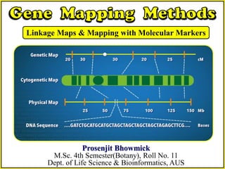
  • 1. Prosenjit Bhowmick M.Sc. 4th Semester(Botany), Roll No. 11 Dept. of Life Science & Bioinformatics, AUS Linkage Maps & Mapping with Molecular Markers
  • 2. A ‘gene’ is a sequence of nucleotides in DNA or RNA that encodes the synthesis of a gene product, either RNA or Protein. The term was coined by Wilhelm Johannsen(1909). The charting of the posotions of genes on a DNA molecule or chromosome and the distance, in linkage units or physical units, between genes is called ‘gene mapping’. INTRODUCTION Gene mapping describes the methods used to identify the locus of a gene and the distances between genes. The essence of all genome mapping is to place a collection of molecular markers onto their respective positions on the genome. Genetic linkage maps allow to determine the position of a gene even when nothing about the gene is known except for its phenotypic effect.  Such maps are often the first step towards isolating the gene responsible for a disease or for a specific trait.
  • 3. HISTORY OF GENE MAPPING Genetics as a branch of biology began in 1866 when Gregor Johann Mendel (1822-1884) described the inheritance pattern of conceptual hereditary units, now, called genes.  In 1902, Boveri-Sutton suggested that chromosomes were the carriers of genetic material. Technique of genetic mapping was first described in 1911 by T. H. Morgan. He noticed that some traits violated Mendel's Law of Independent Assortment. Genetic mapping did not start in humans until the 1950s, because it was hard to know what traits were caused by genetic mutations. With introduction of RFLP(1980s), effort was undertaken to generate maps of all the chromosomes & the first maps were made in 1980s but covered only parts of chromosomes and had few markers.  Maps of whole chromosomes were made by 1980s. By 1990s, a number of whole-genome (i.e., covering all the chromosomes) genetic maps were generated. T. H. Morgan( 1866-1945) Image source: Google images G. J. Mendel (1822-1884)
  • 4. Three different strategies have been used to construct genetic maps. All these strategies offer different levels of resolution at which genomes can be studied. The strategies are: TYPES OF GENE MAPS Gene Mapping Linkage Mapping Cytogenetic Mapping Physical Mapping  Arrangement of gene & DNA markers on a chromosome.  Relative distance between position on a genetic map are calculated using recombinant frequencies  Provide physical distance between landmarks on the chromosome, ideally measured in nucleotide bases.  Map is created by fragmenting the DNA molecule using restriction enzymes and then looking for overlaps
  • 5.  The greater the frequency of recombination (segregation) between two genetic markers, the further apart they are assumed to be.  Conversely, the lower the frequency of recombination between the markers, the smaller the physical distance between them.  Historically, the markers originally used were detectable phenotypes (enzyme production, eye colour) derived from coding DNA sequences.  Eventually, confirmed or assumed noncoding DNA sequences such as microsatellites or those generating RFLPs have been used. LINKAGE MAPPING Linkage is the tendency of DNA sequences that are close together on a chromosome to be inherited together during the meiosis phase of sexual reproduction. A linkage map depicts the order of genetic markers and the relative distances between them as measured in terms of recombination frequencies between the markers.
  • 6.  Recombination frequency is a measure of genetic linkage and it is used in creation of genetic linkage maps.  A centimorgan (cM) is a unit that describes a recombination frequency of 1%.  Using cM as map units , the genetic distance between two loci can be measured, based upon their recombination frequency. RECOMBINATION FREQUENCY Recombination frequency is the frequency with which a single chromosome crossover will take place between two genes during meiosis. Image source: https://isogg.org/wiki/Recombination
  • 7. Example:  Distance between gene b & cn = 9cM (as Recombination frequency is 9%)  Distance between gene cn & vg = 11cM (as Recombination frequency is 11%)  Total Distance between gene b & gene vg= 9cM + 11cM = 20cM MAP UNIT or CENTIMORGAN A map unit or centimorgan is a unit of measure used to approximate the distance between genes. The Morgan unit is named in honour of T. H. Morgan. 1 Map unit or 1 cM = 1% Recombination frequency Image source: https://isogg.org/wiki/Recombination
  • 8. Alfred Henry Sturtevant, a Columbia University undergraduate who was working with Morgan constructed the first Linkage map in 1913. The First Linkage Map Image source: https://www.nature.com/scitable/topicpage/thomas-hunt-morgan-genetic-recombination-and-gene-496/ He has taken four genes & these were present on the X chromosome of the Drosophila melanogaster. By making experimental crosses, he had observed the number of parental and recombinant genotypes among the progenies. The calculated recombination frequencies between these four genes were used to depict the distance between the investigated genes. Recombination frequencies Between m & v = 3.0% Between m & y = 33.7% Between v & w = 29.4% Between w & y = 1.3%
  • 9. As linkage map or genetic map is the outcome of crossing over studies, it is also called as cross over map. The linkage mapping includes the following processes: 1. Determination of Linkage Groups (Mapping Populations). 2. Determination of Map Distance. (a) Two point test cross (b) Three point test cross 3. Determination of Gene Order. 4. Combining Map Segments. 5. Interference & Coincidence CONSTRUCTION OF A LINKAGE MAP
  • 10. Mapping population is a group of individuals used for gene mapping. Selection of appropriate mapping population is fundamental to the success of a gene mapping project. 1. DETERMINATION OF LINKAGE GROUPS Before starting a gene mapping of the chromosome of a species, the exact number of chromosomes must be known. The total number of genes of that species by undergoing hybridization experiments in between wild & mutant strains have to be determined. By the same hybridization technique it can also be determined that how many phenotypic traits remain always linked and consequently their genes during the course of inheritance. And thus the different linkage groups of a species can be determined.
  • 11.  The intergene distance on the chromosome cannot be measured in the customary units employed in light microscopy.  Geneticists use an arbitrary unit to measure the map units, to describe distance between linked genes. 2. DETERMINATION OF MAP DISTANCE A map unit is equal to 1% crossover, i.e. It represents the linear distance along the chromosome for which a recombinant frequency of 1% is observed. Image source: https://isogg.org/wiki/Recombination Example: In this cross the crossover of gamates are Ab(2%) and ab(2%) . Total crossover = 4% (aB%+Ab%) So, distance between A & B will be 4 cM or map unit.
  • 12. 2(a) TWO POINT TEST CROSS The % of crossing over between two linked genes is calculated by a two point test cross. Example: In this dihybrid test cross the Ac/ac(13%) & aC/ac(13%) were produced from the crossover gametes from the dihybrid parents. Thus 26 % (13% + 13%) of the gamates are cross over types. So distance between the loci A & C is estimated to be 26 cM As double crossover do not occur between genes less then 5cM apart, so for genes farther apart 3 point test cross is used.
  • 13. 2(a) THREE POINT TEST CROSS A three point test cross gives us the linear order in which three genes should be present on chromosome. Example: In addition to the previous A & C genes, let us assume gene B, located in close proximity in the same linkage group. A trihybrid cross of ABC/ABC & abc/abc produced F1 hybrid ABC/abc and its test cross with recessive parent abc/abc produced following offsprings: Three Point test cross results (Btw. F1 hybrid ABC/abc & Recessive parent abc/abc) 36% ABC/abc 36% abc/abc 9% Abc/abc 9% aBC/abc 4% ABc/abc 4% abC/abc 1% AbC/abc 1% aBc/abc 72% Parental Type 18% Single crossovers (Btw. A & B)-Region1 8% Single crossovers (Btw. B & C)-Region 2 2% Double crossover To measure distance between two genes we add all double and single crossovers(CO) Distance between A-B: 18% single C.O.+ 2% double C.O.= 20% = 20 cM Distance between B-C: 8% single C.O.+2% double C.O.= 10% = 10 cM Distance between A-C: A-B(20cM) + B-C(10cM) = 30 cM apart A-C
  • 14. 3. DETERMINATION OF GENE ORDER After determining the relative distance between genes of a linkage group, it becomes easy to place genes in their proper linear order. Example: If we suppose the distance between genes A-B=12cM, B-C=7cM, A-C= 5cM, we can determine the order of gene in the following manner: B 12 cM A A 5 cM C B 7 cM C A 12 cM B A 5 cM C B 7 cM C A 12 cM B A 5 cM C C 7 cM B Case 1: Gene order = B-A-C Incorrect: Distance between B-C are not equitable Case 2: Gene order = A-B-C Incorrect: Distance between A-C are not equitable Case 3: Gene order =B-C-A Correct: Distance between A-B are equitable & gene C must be in centre.
  • 15. 4. COMBINING MAP SEGMENTS Finally, the different segments of maps of a complete chromosome are combined to form a complete genetic map. Example: We can combine the different segments of the previous example into a single map by using simple calculation. A 12 cM B A 5 cM C C 7 cM B Case 3: Gene order =B-C-A Correct: Distance between A-B are equitable & gene C must be in centre. As A-C distance = 5 cM & B-C distance = 7 cM; and by ordering the genes we know gene C is in between A & B, so we can combine the map putting C in betwwen(5cM from A & 7cM from B) A 5 cM C 7cM b
  • 16. 4. COMBINING MAP SEGMENTS Finally, the different segments of maps of a complete chromosome are combined to form a complete genetic map. Example: We can combine the different segments of the previous example into a single map by using simple calculation. A 12 cM B A 5 cM C C 7 cM B Case 3: Gene order =B-C-A Correct: Distance between A-B are equitable & gene C must be in centre. As A-C distance = 5 cM & B-C distance = 7 cM; and by ordering the genes we know gene C is in between A & B, so we can combine the map putting C in betwwen(5cM from A & 7cM from B) A 5 cM C 7cM b
  • 17. 5. INTERFERENCE & COINCIDENCE In higher organisms , one chisma formation reduces the probability of anthother chisma formation in an immediately adjacent region. The tendency of one crossover to interfere with the other is called interference. Centromere shows similar interference effect. The net result of this interference is, fewer double crossover then expected according to map distances. Interference is expressed in terms of coefficient of coincidence. When interference is complete(1.0), no double crossover will be observed and coincidence becomes 0. Coincidence + Interference = 1.0
  • 18. A molecular marker is a DNA sequence used for chromosome mapping as it can be located at a specific site in a chromosome. MOLECULAR MARKERS Molecular Marker Biochemical Isozymes DNA Based Markars Hybridization Based 1. RFLP 2. Minisatellite 3. Microsatellite PCR Based 1. RAPD 2. AFLP 3. STS First Generation: 1980s Based on DNA-DNA hybridizations, such as RFLP. Second Generation: 1990s Based on PCR: •Using random primers: RAPD •Using specific primers: STS Based on PCR and restriction cutting: AFLP Third Generation: recently Based on DNA point mutations (SNP)
  • 19.  This has been particularly important with two types of organisms - microbes and humans.  Microbes, such as bacteria and yeast, have very few visual characteristics so gene mapping with these organisms has to rely on biochemical phenotypes.  A big advantage is that relevant genes have multiple alleles.  For example- Gene called HLA-DRB1 has at least 290 alleles and HLA-B has over 400 alleles. BIOCHEMICAL MARKERS IN LINKAGE MAPPING
  • 20.  Genes are very useful markers but they are by no means ideal.  Mapped features that are not genes are called DNA markers.  A DNA marker must have at least two alleles to be useful.  DNA sequence features that satisfy this requirement are- DNA MARKERS FOR LINKAGE MAPPING Restriction Fragment Length Polymorphism (RFLPs) Simple Sequence Length Polymorphism (SSLPs) Single Nucleotide Polymorphism (SNPs)
  • 21. RFLP TECHNIQUE IN GENE MAPPING RFLPs(Restriction fragment length polymorphisms) were the first type of DNA marker to be studied for linkage mapping.. Restriction enzymes cut DNA molecules at specific recognition sequences. But restriction sites in genomic DNA are polymorphic and exists as two alleles.  One allele displaying the correct sequence for the restriction site and therefore being cut when the DNA is treated with the enzyme.  The second allele having a sequence alteration so the restriction site is no longer recognized. The RFLP and its position in the genome map can be worked out following the inheritance of its alleles.
  • 22. The DNA molecule on the left has a polymorphic restriction site (marked with the asterisk) that is not present in the molecule on the right. The RFLP is revealed after treatment with the restriction enzyme because one of the molecules is cut into four fragments whereas the other is cut into three fragments. In order to score an RFLP, it is necessary to determine the size of just one or two individual restriction fragments against a background of many irrelevant fragments. Image source: T. A. Brown (2006), GENOMICS 3 (3rd Edition)
  • 23. There are two methods for scoring an RFLP: 1. Southern hybridization 2. PCR 1. Southern hybridization: i. The DNA is digested with the appropriate restriction enzyme and separated in an agarose gel. ii. The smear of restriction fragments is transferred to a nylon membrane and probed with a piece of DNA that spans the polymorphic restriction site. iii. If the site is absent then a single restriction fragment is detected (lane 2) iv. if the site is present then two fragments are detected (lane3) Image source: T. A. Brown (2006), GENOMICS 3 (3rd Edition)
  • 24. 2. RFLP typing by PCR: i. using primers that anneal either side of the polymorphic restriction site. ii. After the PCR, the products are treated with the appropriate restriction enzyme and then analyzed by agarose gel electrophoresis. iii. If the site is absent then one band is seen on the agarose gel; if the site is present then two bands are seen. Image source: T. A. Brown (2006), GENOMICS 3 (3rd Edition)
  • 25. SSLPs IN GENE MAPPING SSLPs(Simple Sequence Length Polymorphism) are arrays of repeat sequences that display length variation. Here different alleles contain different number of repeat sequences. Two types of SSLPs are: 1. Minisatellites (VNTRs) repeat unit is up to 25 bp in length 2. Microsatellites (STRs) Shorter units, dinucleotide or tetranucleotide units SSLPs can be multiallelic. In allele 1 the motif 'GA' is repeated three times, and in allele 2 it is repeated five times. Microsatellites are more popular than minisatellites as DNA markers. Image source: T. A. Brown (2006), GENOMICS 3 (3rd Edition)
  • 26. SSLP typing by PCR: The region surrounding the SSLP is amplified and the products loaded into lane A of the agarose gel. Lane B contains DNA markers that show the sizes of the bands given after PCR of the two alleles. The band in lane A is the same size as the larger of the two DNA markers, showing that the DNA that was tested contained allele 2. Image source: T. A. Brown (2006), GENOMICS 3 (3rd Edition)
  • 27. SNPs IN GENE MAPPING There are some positions in the genome where some individuals have one nucleotide while others have another. Some SNPs give rise to RFLPs but many do not. SNPs originate when a point mutation occurs in a genome converting one nucleotide to another. There are just two alleles- the original sequence and the mutated version. SNPs enable very detailed genome maps to be constructed. Image source: T. A. Brown (2006), GENOMICS 3 (3rd Edition)
  • 28. Detecting an SNP by solution hybridization: The oligonucleotide probe has two end-labels. One of these is a fluorescent dye and the other is a quenching compound. The two ends of the oligonucleotide basepair to one another, so the fluorescent signal is quenched. When the probe hybridizes to its target DNA, the ends of the molecule become separated, enabling the fluorescent dye to emit its signal. The two labels are called 'molecular beacons'. Image source: T. A. Brown (2006), GENOMICS 3 (3rd Edition)
  • 29. Detecting an SNP by Oligonucleotide Ligation Assay: An oligonucleotide is a short single-stranded DNA molecule, usually less than 50 nucleotides in length, that is synthesized in the test tube. If conditions are right, then an oligonucleotide will hybridize with another DNA molecule only if the oligonucleotide forms a completely base-paired structure with the other. If there is a single mismatch - a single position within the oligonucleotide that does not form a base pair, then hybridization does not occur. Oligonucleotide hybridization can therefore discriminate between the two alleles of an SNP. Image source: T. A. Brown (2006), GENOMICS 3 (3rd Edition)
  • 30. Process of Linkage Mapping Using Molecular Markers We can map RFLPs and other molecular markers by making crosses between two parents differing for two or more RFLPs and scoring the progeny for these RFLP markers. Explanation: Lets us suppose that, 1. One RFLP is detected with probe *1 and gives bands of 5kb and 6kb indifferent strains. 2. Similarly the second RFLP is detected by probe *2 and yields bands of 2kb and 3kb. The mapping of these two RFLP markers may be done as follows: 1. Two strains that are homozygous for the two RFLP markers, e.g. One shows bands of 5kb & 3kb, while the other shows 6kb & 2kb bands are crossed together.
  • 31. 2. The F1 so obtained shows all the four bands. The F1 is back crossed with one of the parent having 6 & 2kb bands. 3. The resulting back-cross progeny are scored for these RFLP bands & each progeny will yield 1 of the 4 band patterns. 4. If the two RFLP markers were not linked, equal proportion of progeny will be present in these 4 categories. 5. But, incase of linkage the proportion of parental progeny will be much higher then the recombinant progeny. Image source: P.S. Cerma(2012), Cell biology and Genetics
  • 32. The LOD Score In actual analysis of RFLP data, linkage is detected by a statistical test called the lod [Logarithm(base 10) of odds] score method developed by Morton in 1955. The LOD score is calculated as follows: If the lod score equals +3 or is greater, the two RFLP markers are considered to be linked. A LOD score less than -2.0 is considered evidence to exclude linkage. If the lod score indicates the two RFLP markers to be linked, then the recombination frequency is calculated to obtain the map distance in terms of map units or cM. Using this map distance data the linkage map (RFLP map) is prepared.
  • 33. PHYSICAL MAPPING In a physical map, genes are depicted in the same order as they occur in chromosome. The distance between genes are shown as number of base pairs separating genes. It uses techniques such as Restriction mapping, FISH etc. Example: Genes sc & w are separated by 1.5x10⁶ bp. Physical mapping usually requires the: 1. Cloning of many pieces of chromosomal DNA. 2. Characterization of these fragments of size, i.e. Length in base pairs & genes present in them. 3. Determination of their relative location along a chromosome (e.g., by FcFISH).
  • 34. CYTOGENETIC MAPPING A cytogenetic map depicts the location of various genes in a chromosome relative to specific microscopically visible landmarks. Each chromosome has a banding pattern, which may be either naturally present or generated by specific staining protocol. In most species, cytogenetic mapping is accurate within limits of approx. 5 megabase pairs(Mb=1000000 bp) along a chromosome. Image source: https://isogg.org/wiki/Recombination
  • 35. Application/Uses of Linkage Maps Studying genome structures, organization and evolution. Estimation of gene effects of important agronomic traits. Tagging genes of interest to facilitate marker assisted selection (MAS) programs. Map based cloning. Identify genes responsible for traits: Plants or Animals Disease resistance. Meat or milk production, etc.
  • 36. Limitations of Linkage Mapping A map generated by linkage technique is rarely sufficient for directing the sequencing phase of a genome project. This is for two reasons: 1. The resolution of a genetic map depends upon the number of crossovers that have been scored.  Genes that are several kb apart may appear at the same position on the linkage map. 2. Genetic maps have limited accuracy. Presence of recombination hotspots means that crossover are more likely to occur at same points rather than at others. Physical mapping technique have been developed to address this problem.
  • 37. CONCLUSION  Linkage mapping is entirely based upon recombination frequency and LOD analysis. Analysing a LOD score is a critical problem in case of large maps. Although by using linkage maps we can determine the distance between two genes and by using three point test cross we can determine the relative locations of genes. The accuracy of linkage maps is a big question and to overcome this issue introduction of physical and cytogenetic mappings were introduced. All molecular markers are not equal and none is ideal. Some are better for some purposes than others. However, all are generally preferable over morphological markers for mapping and marker assisted selection.
  • 38. REFERENCES B. D. Singha (2012), Biotechnology: Expanding horizons (4th Revised edition); Kalyani Publishers, New Delhi; ISBN: 9789327222982; Pages(112- 146). Boris M. Sharga et. Al (2018), Practical 6. Genetic linkage and mapping. P. K. Gupta(2015), Cytology & Genetics (7th Edition), Rastogi Publisher; ISBN: 9788171330473; Pages 72-97). Paul H Dear(2001), Genome Mapping, ENCYCLOPEDIA OF LIFE Sciences, Macmillan Publishers Ltd, Nature Publishing Group. P. S. Verma & V. K. Agarwal (2012), Cell biology, Genetics, Molecular biology, Evolution & Ecology(14th Edition);S. Chand (P) Ltd.; ISBN: 8121924421; Pages(84-113). T. A. Brown (2006), GENOMICS 3 (3rd Edition);Garland Science; ISBN- 10:0815341385; Pages(255-286).