Formulario de Trigonometría.

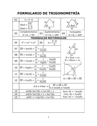
1. 1
FORMULARIO DE TRIGONOMETRÍA
01 S = θ ⋅ R
1Rad =
360°
2 ⋅ π
1Rad = 57.3°
02
Complementarios
03
Suplementarios
04
Conjugados
θ + θc = 90° θ + θs = 180° θ + θk = 360°
TRIÁNGULOS RECTÁNGULOS
05 h2
= co2
+ ca2
06 A =
B ⋅ H
2
B = Base = ca
H = Altura = co
R = OB
̅̅̅̅ = OC
̅̅̅̅ = OE
̅̅̅̅
07 AB
̅̅̅̅ = Sen(θ) =
co
h
=
1
Csc(θ)
08 OA
̅̅̅̅ = Cos(θ) =
ca
h
=
1
Sec(θ)
09 CD
̅̅̅̅ = Tan(θ) =
co
ca
=
1
Ctg(θ)
=
Sen(θ)
Cos(θ)
10 EF
̅
̅̅
̅ = Ctg(θ) =
ca
co
=
1
Tan(θ)
=
Cos(θ)
Sen(θ)
11 OD
̅̅̅̅ = Sec(θ) =
h
ca
=
1
Cos(θ)
12 OF
̅̅̅̅ = Csc(θ) =
h
co
=
1
Sen(θ)
Si θ ≅ 0 Rad ⇒ {
BC
̅̅̅̅ ≅ AB
̅̅̅̅ ≅ CD
̅̅̅̅
S ≅ Sen(θ) ≅ Tan(θ)
13 ⊿OAB: Sen2
(θ) + Cos2
(θ) = 1 Sen(−θ) = −Sen(θ)
Cos(−θ) = Cos(θ)
Tan(−θ) = −Tan(θ)
14 ⊿OCD: Tan2
(θ) + 1 = Sec2
(θ)
15 ⊿OEF: 1 + Ctg2
(θ) = Csc2
(θ)

2. 2
16 θ = ω ⋅ t
{
x = Cos(t)
y = Sen(t)
x2
+ y2
= 1
17 {
x = Cos(ω ⋅ t)
y = Sen(ω ⋅ t)
18 x2
+ y2
= 1
19 Sen(θ) = θ −
θ3
6
+
θ5
120
−
θ7
5040
+ ⋯
20 Cos(x) = 1 −
θ2
2
+
θ4
24
−
θ6
720
+ ⋯
TRIÁNGULOS OBLICUÁNGULOS
21 α + β + γ = 180°
22
Ley de Senos:
a
Sen(α)
=
b
Sen(β)
=
c
Sen(γ)
= 2 ⋅ Rc
23
Ley de Cosenos:
a2
= b2
+ c2
− 2 ⋅ b ⋅ c ⋅ Cos(α)
b2
= a2
+ c2
− 2 ⋅ a ⋅ c ⋅ Cos(β)
c2
= a2
+ b2
− 2 ⋅ a ⋅ b ⋅ Cos(γ)
24
Ley de Cosenos:
α = ∢Cos (
a2
− b2
− c2
−2 ⋅ b ⋅ c
)
β = ∢Cos (
b2
− a2
− c2
−2 ⋅ a ⋅ c
)
γ = ∢Cos (
c2
− a2
− b2
−2 ⋅ a ⋅ b
)
25
Ley de las Proyecciones:
a = b ⋅ Cos(γ) + c ⋅ Cos(β)
b = a ⋅ Cos(γ) + c ⋅ Cos(α)
c = a ⋅ Cos(β) + b ⋅ Cos(α)

3. 3
26
Ri = (
−a + b + c
2
) ⋅ Tan (
α
2
)
Ri = (
a − b + c
2
) ⋅ Tan (
β
2
)
Ri = (
a + b − c
2
) ⋅ Tan (
γ
2
)
(06) A =
B ⋅ H
2
27 A =
a ⋅ b
2
⋅ Sen(γ) =
a ⋅ c
2
⋅ Sen(β) =
b ⋅ c
2
⋅ Sen(α)
28 A =
1
4
⋅ √(a + b + c) ⋅ (−a + b + c) ⋅ (a − b + c) ⋅ (a + b − c)
IDENTIDADES TRIGONOMÉTRICAS
29
Identidades Trigonométricas Pitagóricas:
Sen2
(θ) + Cos2
(θ) = 1
Tan2
(θ) + 1 = Sec2
(θ)
1 + Ctg2
(θ) = Csc2
(θ)
30 Sen(α + β) = Sen(α) ⋅ Cos(β) + Cos(α) ⋅ Sen(β)
31 Sen(α − β) = Sen(α) ⋅ Cos(β) − Cos(α) ⋅ Sen(β)
32 Cos(α + β) = Cos(α) ⋅ Cos(β) − Sen(α) ⋅ Sen(β)
33 Cos(α − β) = Cos(α) ⋅ Cos(β) + Sen(α) ⋅ Sen(β)
34 Tan(α + β) =
Tan(α) + Tan(β)
1 − Tan(α) ⋅ Tan(β)
35 Tan(α − β) =
Tan(α) − Tan(β)
1 + Tan(α) ⋅ Tan(β)
36 Sen(2 ⋅ α) = 2 ⋅ Sen(α) ⋅ Cos(α)
37 Cos(2 ⋅ α) = Cos2
(α) − Sen2
(α)
38 Tan(2 ⋅ α) =
2 ⋅ Tan(α)
1 − Tan2(α)
39 Sen(α) ⋅ Cos(β) =
Sen(α + β)
2
+
Sen(α − β)
2
40 Cos(α) ⋅ Sen(β) =
Sen(α + β)
2
−
Sen(α − β)
2
41 Cos(α) ⋅ Cos(β) =
Cos(α + β)
2
+
Cos(α − β)
2

4. 4
42 Sen(α) ⋅ Sen(β) = −
Cos(α + β)
2
+
Cos(α − β)
2
43 Sen(α) + Sen(β) = 2 ⋅ Sen (
α + β
2
) ⋅ Cos (
α − β
2
)
44 Sen(α) − Sen(β) = 2 ⋅ Cos (
α + β
2
) ⋅ Sen (
α − β
2
)
45 Cos(α) + Cos(β) = 2 ⋅ Cos (
α + β
2
) ⋅ Cos (
α − β
2
)
46 Cos(α) − Cos(β) = −2 ⋅ Sen (
α + β
2
) ⋅ Sen (
α − β
2
)
π = lim
N→∞
N ⋅ Tan (
180°
N
) = 3.141592 …
Signos:
Cuadrante: I II III IV
Sen(θ) + + - -
Cos(θ) + - - +
Tan(θ) + - + -
Ctg(θ) + - + -
Sec(θ) + - - +
Csc(θ) + + - -

5. 5
Función y CoFunción: F(θ) = coF(θc)
coSenθ coTanθ coSecθ
θ Senθ Cosθ Tanθ Ctgθ Secθ Cscθ
0° 0 1 0 ∞ 1 ∞
15°
(45-30)
√3 − 1
2 ⋅ √2
√3 + 1
2 ⋅ √2
√3 − 1
√3 + 1
√3 + 1
√3 − 1
2 ⋅ √2
√3 + 1
2 ⋅ √2
√3 − 1
30°
1
2
√3
2
1
√3
√3
2
√3
2
45°
1
√2
1
√2
1 1 √2 √2
60°
√3
2
1
2
√3
1
√3
2
2
√3
75°
(30+45)
√3 + 1
2 ⋅ √2
√3 − 1
2 ⋅ √2
√3 + 1
√3 − 1
√3 − 1
√3 + 1
2 ⋅ √2
√3 − 1
2 ⋅ √2
√3 + 1
90° 1 0 ∞ 0 ∞ 1
Sen:
0° 30° 45° 60° 90°
√0 1 2 3 4
2
Cos:
0° 30° 45° 60° 90°
√4 3 2 1 0
2
Tan:
0° 30° 45° 60° 90°
√0 1 2 3 4
√4 3 2 1 0

6. 6
TRIGONOMETRÍA HIPERBÓLICA
47 Senh(x) =
℮x
− ℮−x
2
48 Cosh(x) =
℮x
+ ℮−x
2
49 Tanh(x) =
℮x
− ℮−x
℮x + ℮−x
=
Senh(x)
Cosh(x)
50 Ctgh(x) =
℮x
+ ℮−x
℮x − ℮−x
=
Cosh(x)
Senh(x)
=
1
Tanh(x)
x ≠ 0
51 Sech(x) =
2
℮x + ℮−x
=
1
Cosh(x)
52 Csch(x) =
2
℮x − ℮−x
=
1
Senh(x)
x ≠ 0
53 Si: y = Senh(x) =
℮x
− ℮−x
2
⇒ x = invSenh(y) = Ln (y + √y2 + 1)
54
Cosh2
(x) − Senh2
(x) = 1
1 − Tanh2
(x) = Sech2
(x)
Ctgh2
(x) − 1 = Csch2
(x)
{
x = Cosh(t)
y = Senh(t)
x2
− y2
= 1
55
Senh(−x) = −Senh(x)
Cosh(−x) = Cosh(x)
Tanh(−x) = −Tanh(x)
56 invSenh(x) = Ln (x + √x2 + 1)
57 invCosh(x) = Ln (x + √x2 − 1) x ≥ 1
58 invTanh(x) =
1
2
⋅ Ln (
1 + x
1 − x
) x2
< 1
59 invCtgh(x) =
1
2
⋅ Ln (
x + 1
x − 1
) x2
> 1
60 invSech(x) = Ln (
1 + √1 − x2
x
) 0 < x ≤ 1

7. 7
61 invCsch(x) = Ln (
1
x
+
√x2 + 1
|x|
) x ≠ 0
℮ = lim
N→∞
(1 +
1
N
)
N
= 2.718281 …
TRIGONOMETRÍA VECTORIAL
62 A
⃗
⃗ = (ax, ay, az) 63 A
⃗
⃗ = ax ⋅ î + ay ⋅ ĵ + az ⋅ k
̂
64 |A
⃗
⃗ | = √ax
2 + ay
2 + az
2 65 {
î = (1,0,0)
ĵ = (0,1,0)
k
̂ = (0,0,1)
66
Cosenos Directores.
{
Cos(αx) =
ax
|A
⃗
⃗ |
Cos(αy) =
ay
|A
⃗
⃗ |
Cos(αz) =
az
|A
⃗
⃗ |
68
Vector Unitario.
A
̂ =
A
⃗
⃗
|A
⃗
⃗ |
A
̂ =
(ax, ay, az)
|A
⃗
⃗ |
A
̂ = (
ax
|A
⃗
⃗ |
,
ay
|A
⃗
⃗ |
,
az
|A
⃗
⃗ |
)
67 Cos2(αx) + Cos2
(αy) + Cos2(αz) = 1
69
Producto PUNTO.
A
⃗
⃗ ⊡ B
⃗
⃗ = (ax, ay, az) ⊡ (bx, by, bz) = {
ax ⋅ bx + ay ⋅ by + az ⋅ bz
|A
⃗
⃗ | ⋅ |B
⃗
⃗ | ⋅ Cos(γ)
70
Producto CRUZ.
A
⃗
⃗ ⊠ B
⃗
⃗ = (ax, ay, az) ⊠ (bx, by, bz) = [
î ĵ k
̂
ax ay az
bx by bz
]
71 |A
⃗
⃗ ⊠ B
⃗
⃗ | = |A
⃗
⃗ | ⋅ |B
⃗
⃗ | ⋅ Sen(γ)
72 Area =
|A
⃗
⃗ ⊠ B
⃗
⃗ |
2
=
|A
⃗
⃗ | ⋅ |B
⃗
⃗ | ⋅ Sen(γ)
2

8. 8
73
Producto Mixto.
Volumen = (A
⃗
⃗ ⊠ B
⃗
⃗ ) ⊡ C
⃗
Volumen = [
ax ay az
bx by bz
cx cy cz
]
74
|A
⃗
⃗ ⊠ B
⃗
⃗ |
A
⃗
⃗ ⊡ B
⃗
⃗
= Tan(γ)
75
Proyección (o componente) de A
⃗
⃗ sobre B
⃗
⃗ .
A
⃗
⃗ B = (A
⃗
⃗ ⊡ B
̂) ⋅ B
̂
Elaboró: MCI José A. Guasco.
https://www.slideshare.net/AntonioGuasco1/