Power systems can be modeled and analyzed using per-unit representations of components. Key models include:
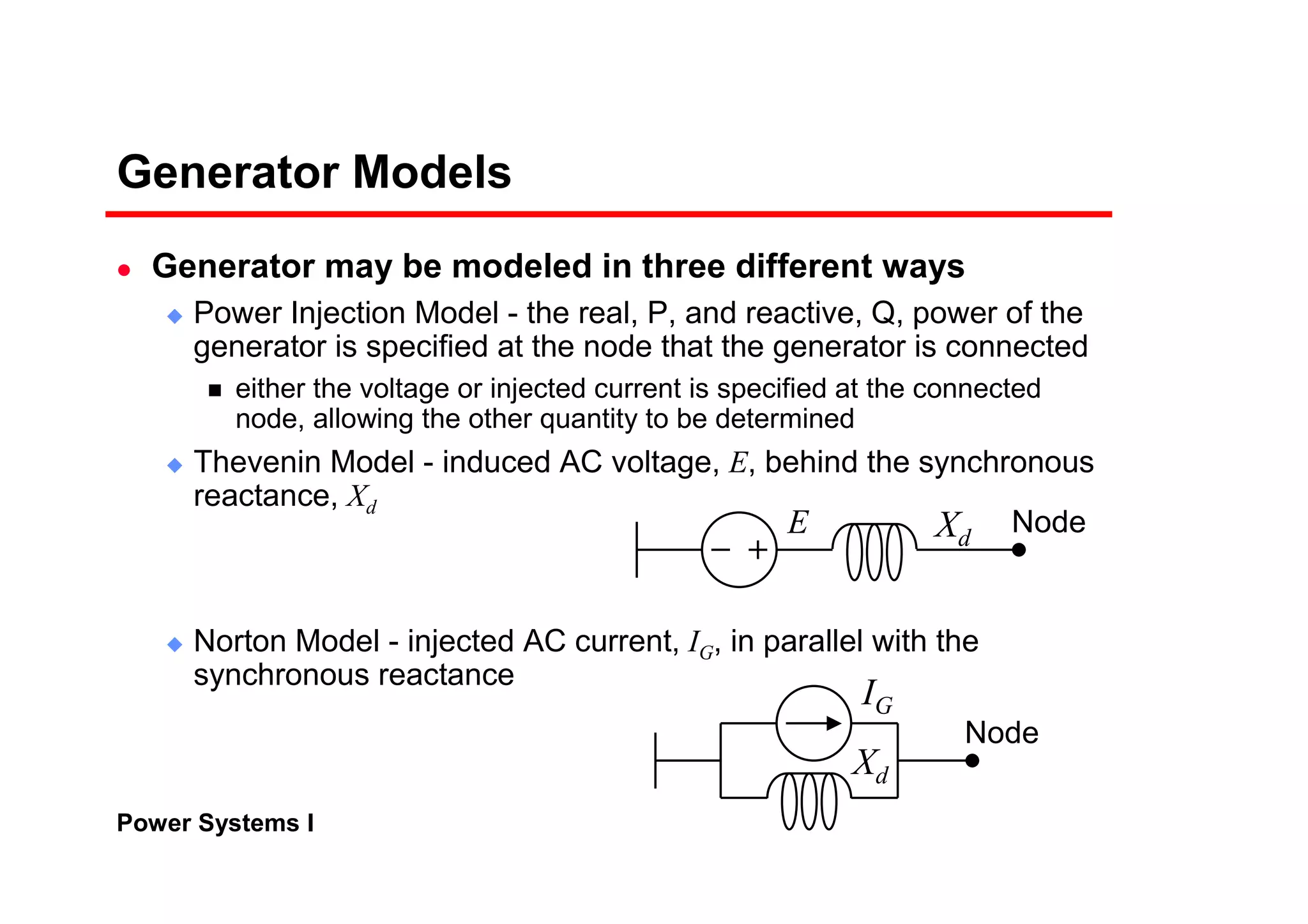
1) Generator models that specify real and reactive power injection or terminal voltage and current.
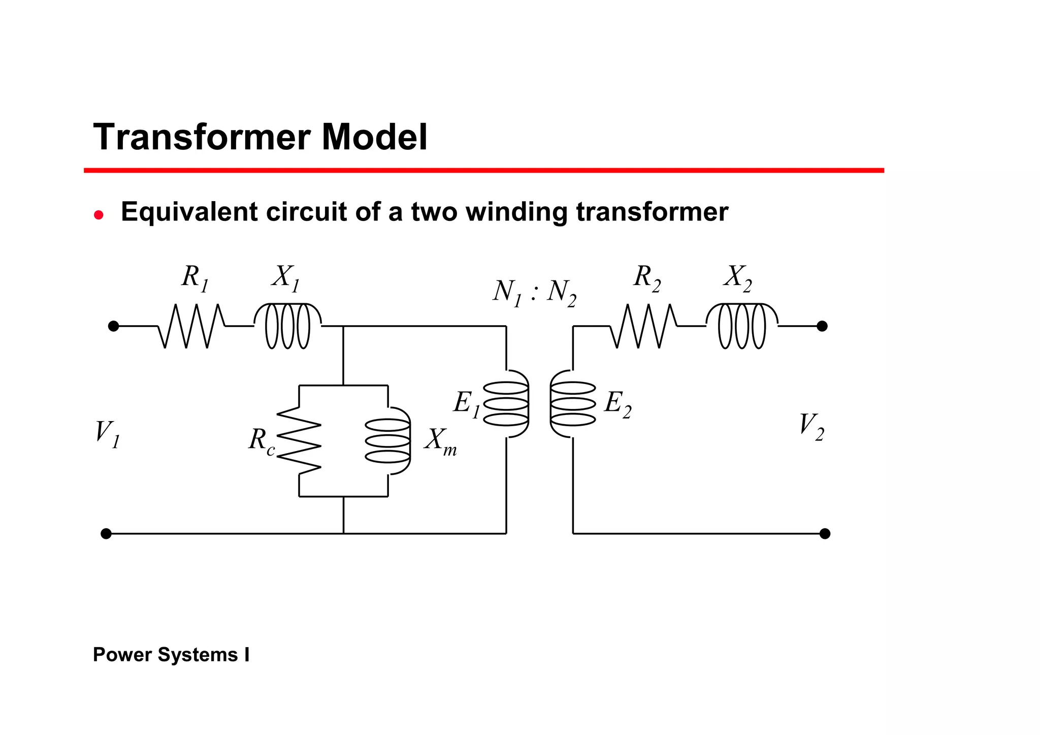
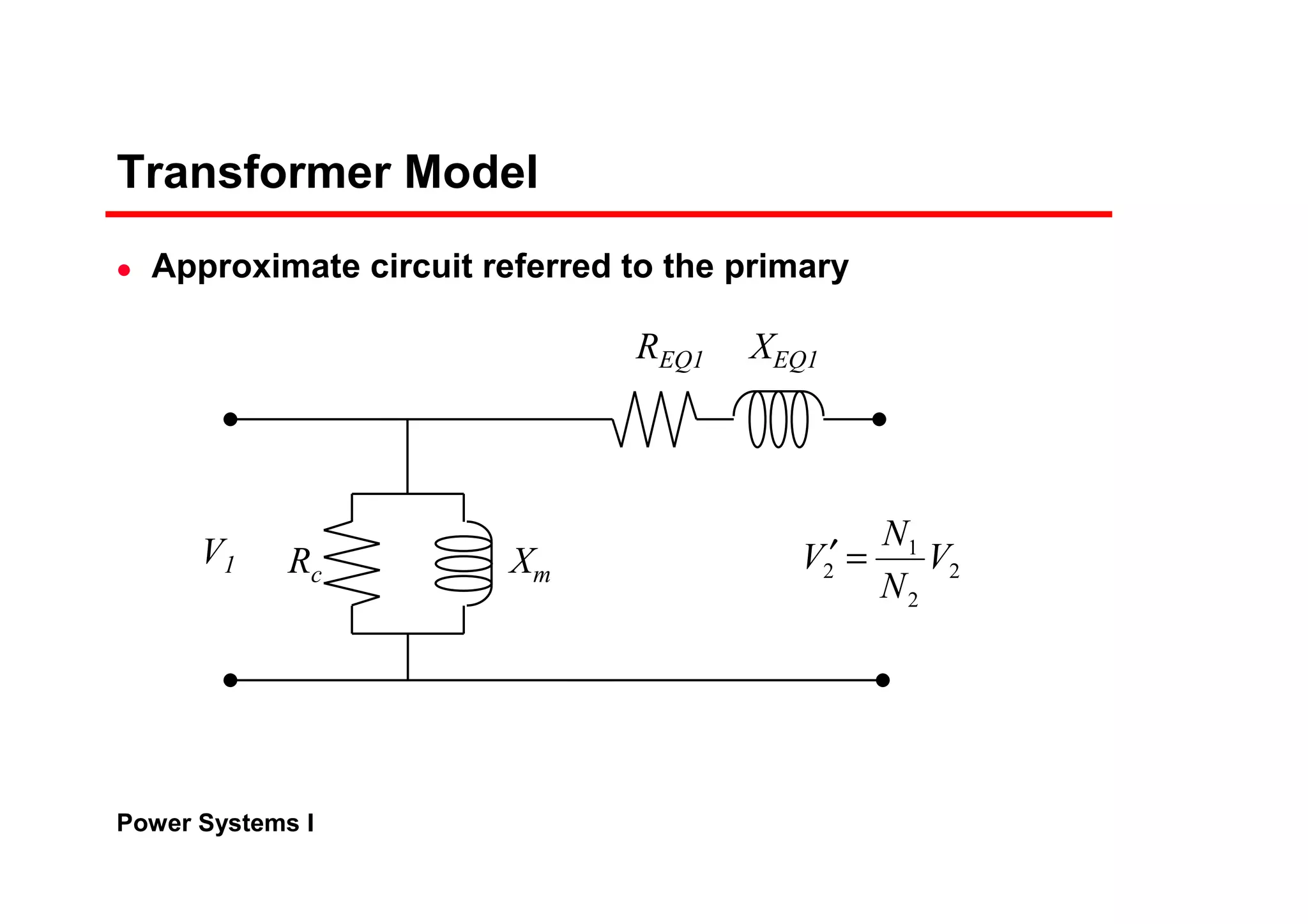
2) Transformer models using an equivalent circuit with magnetizing reactance and resistance.
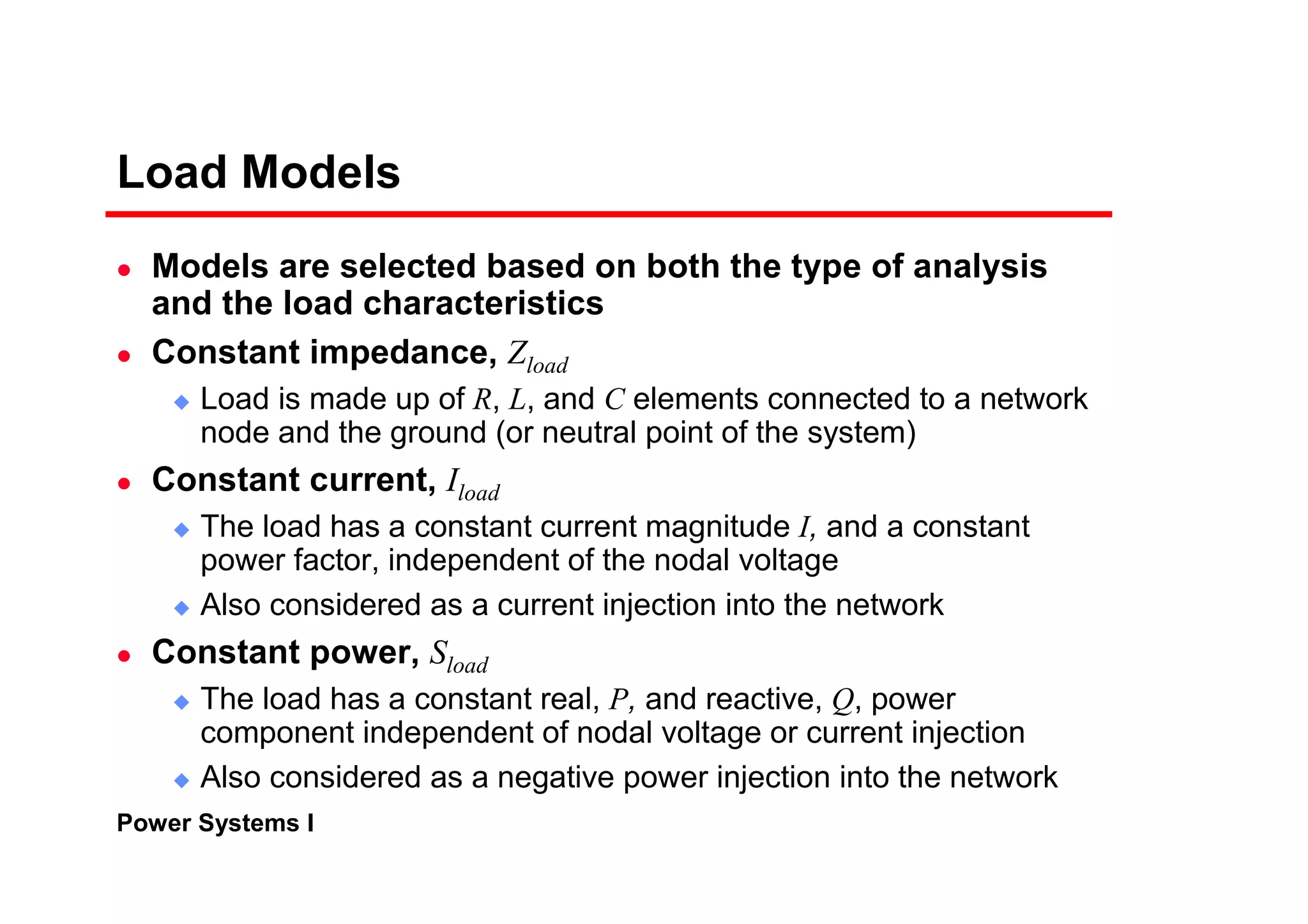
3) Load models like constant impedance, current, or power to represent different load characteristics.
4) Transmission lines modeled as series impedances.
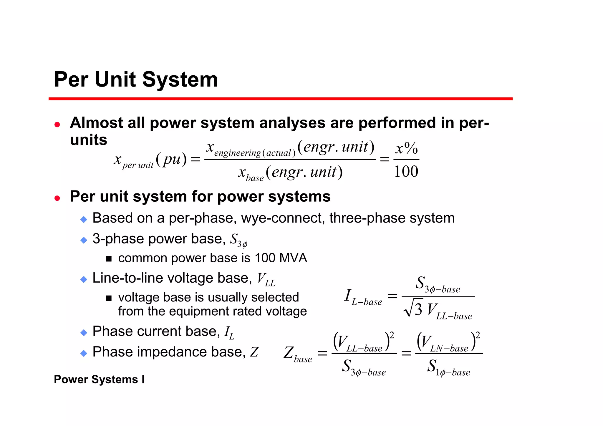
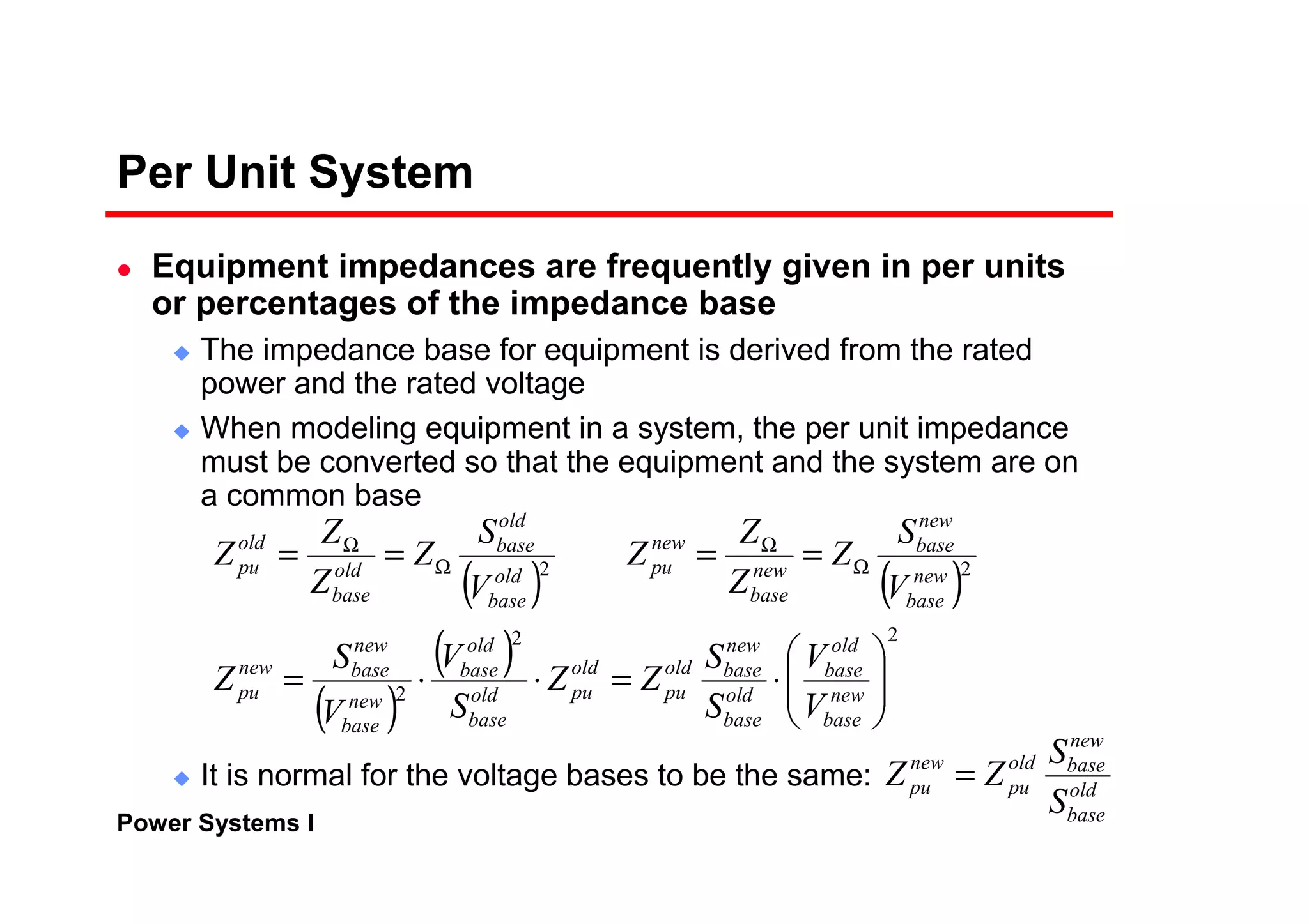
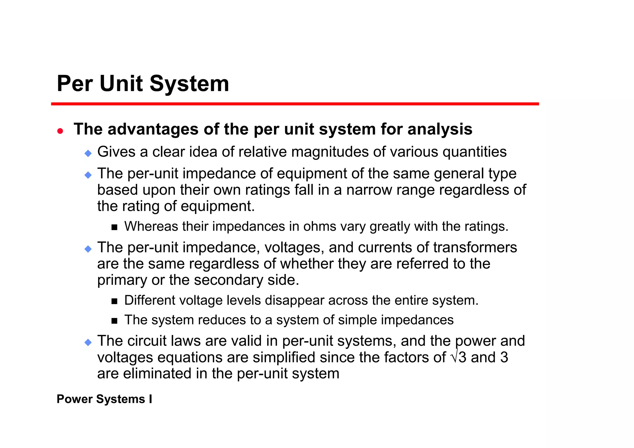
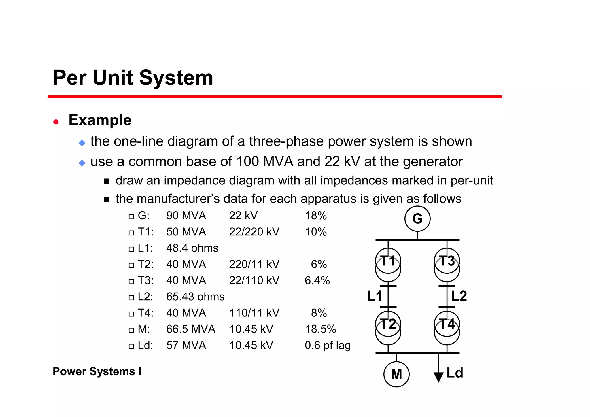
The per-unit system allows analysis of different voltage levels on a common scale and simplifies modeling of components.
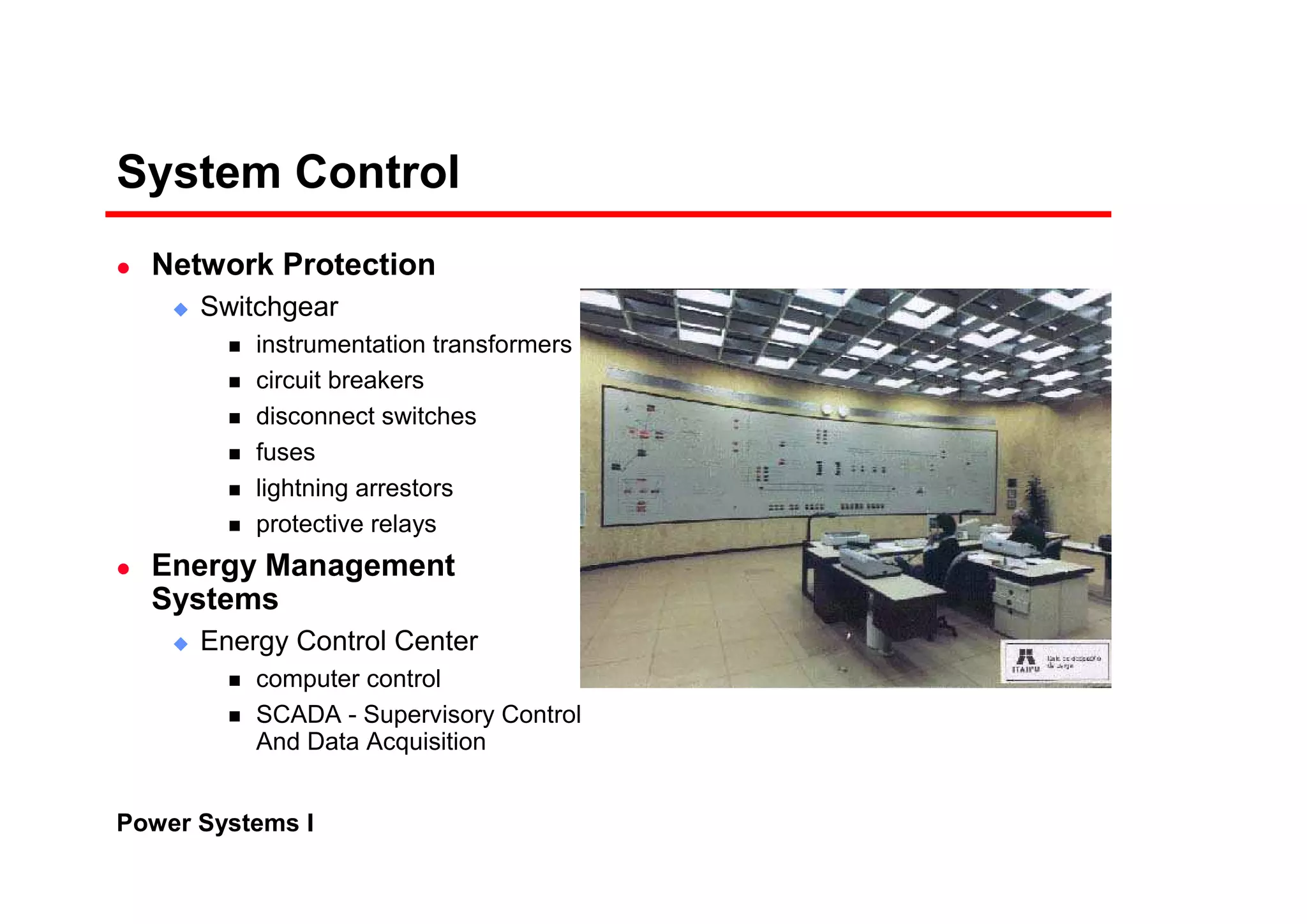
![Power Systems I
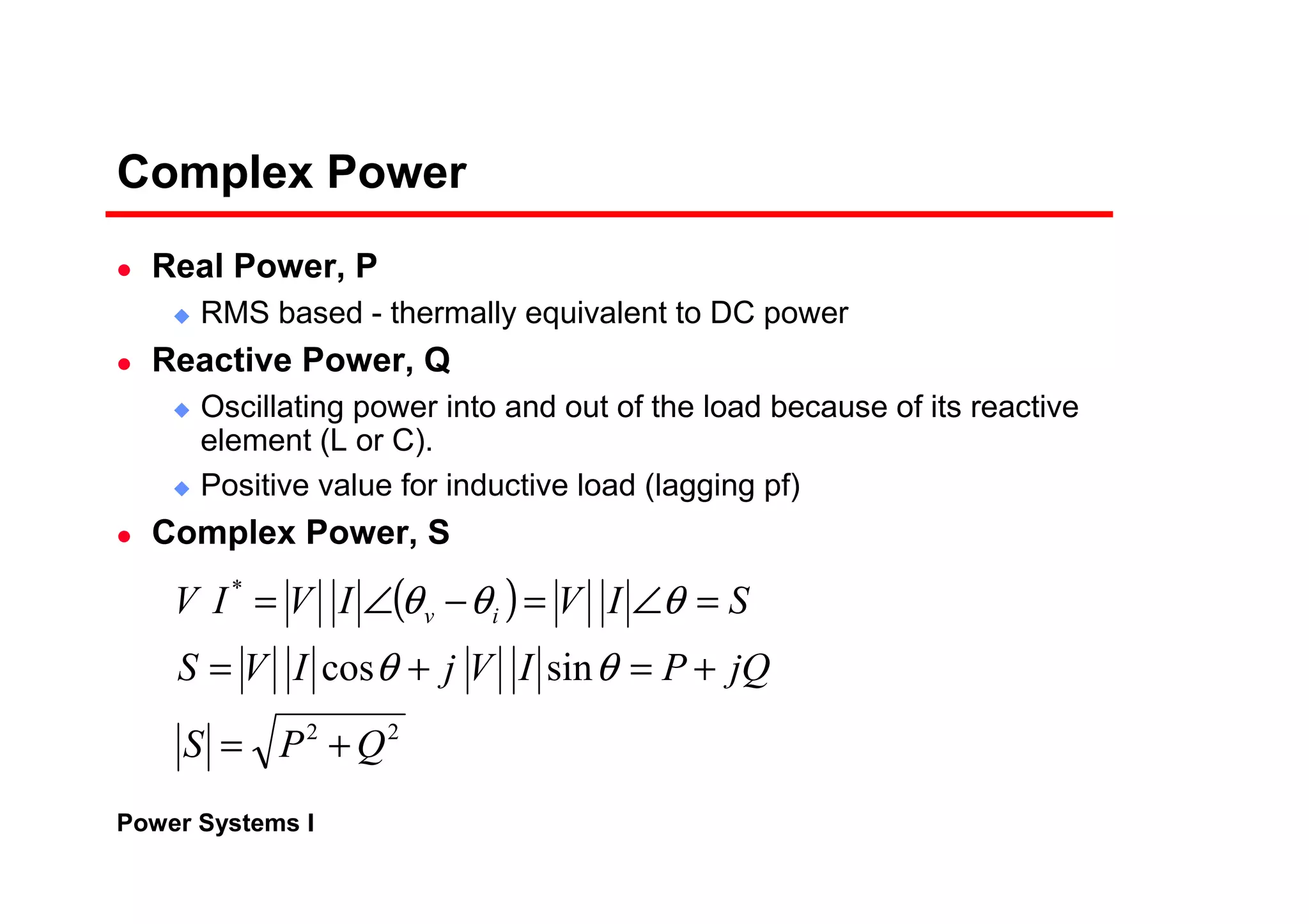
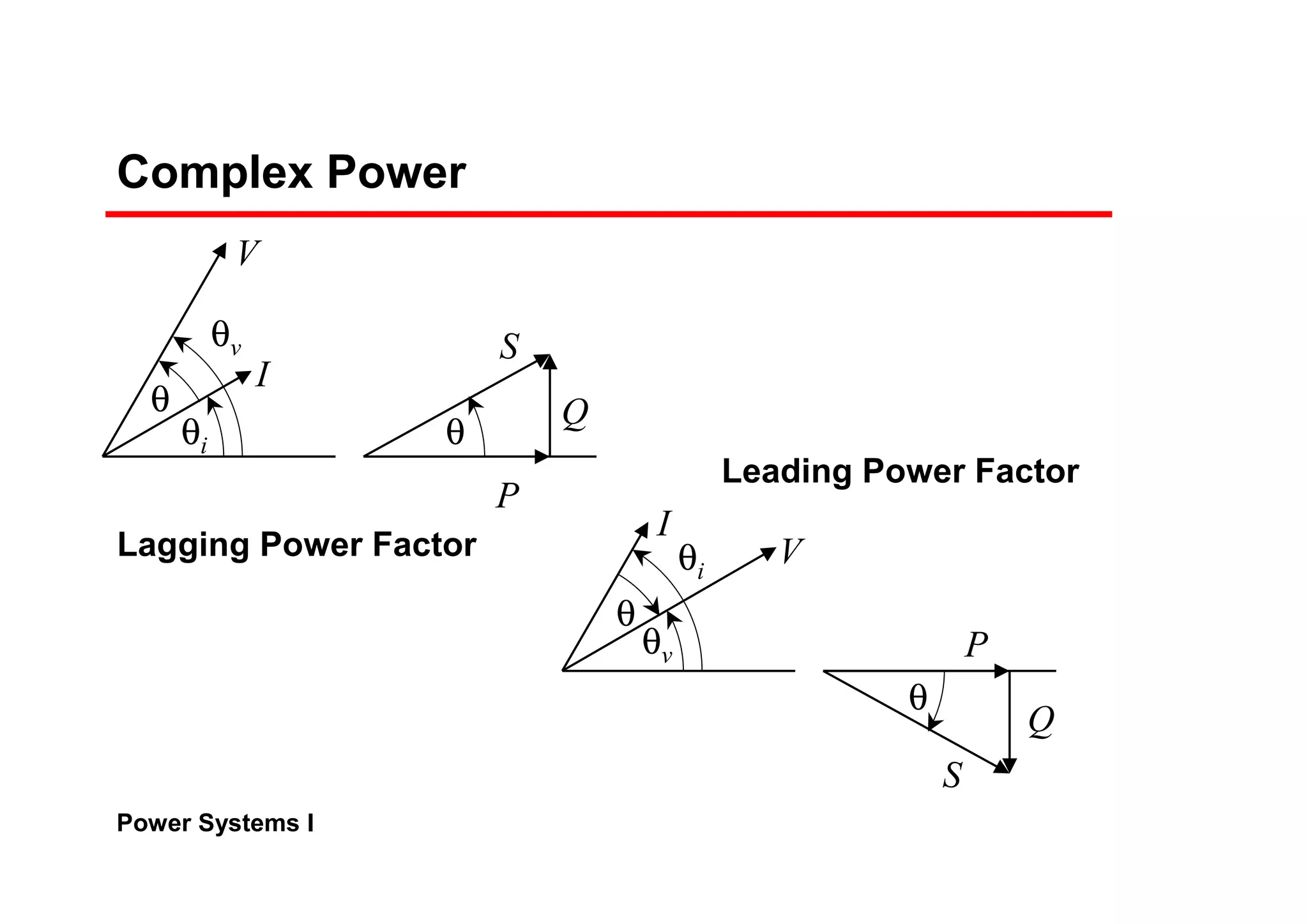
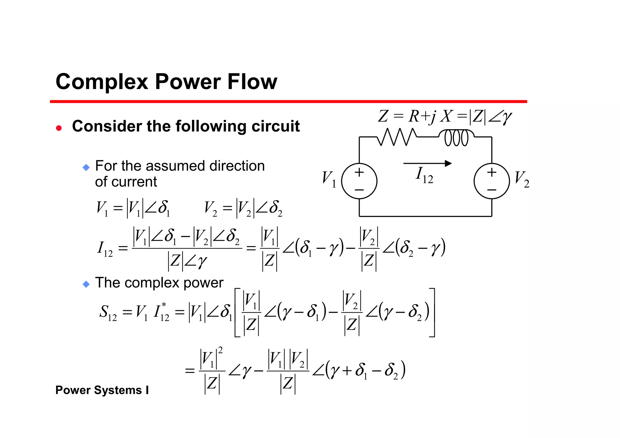
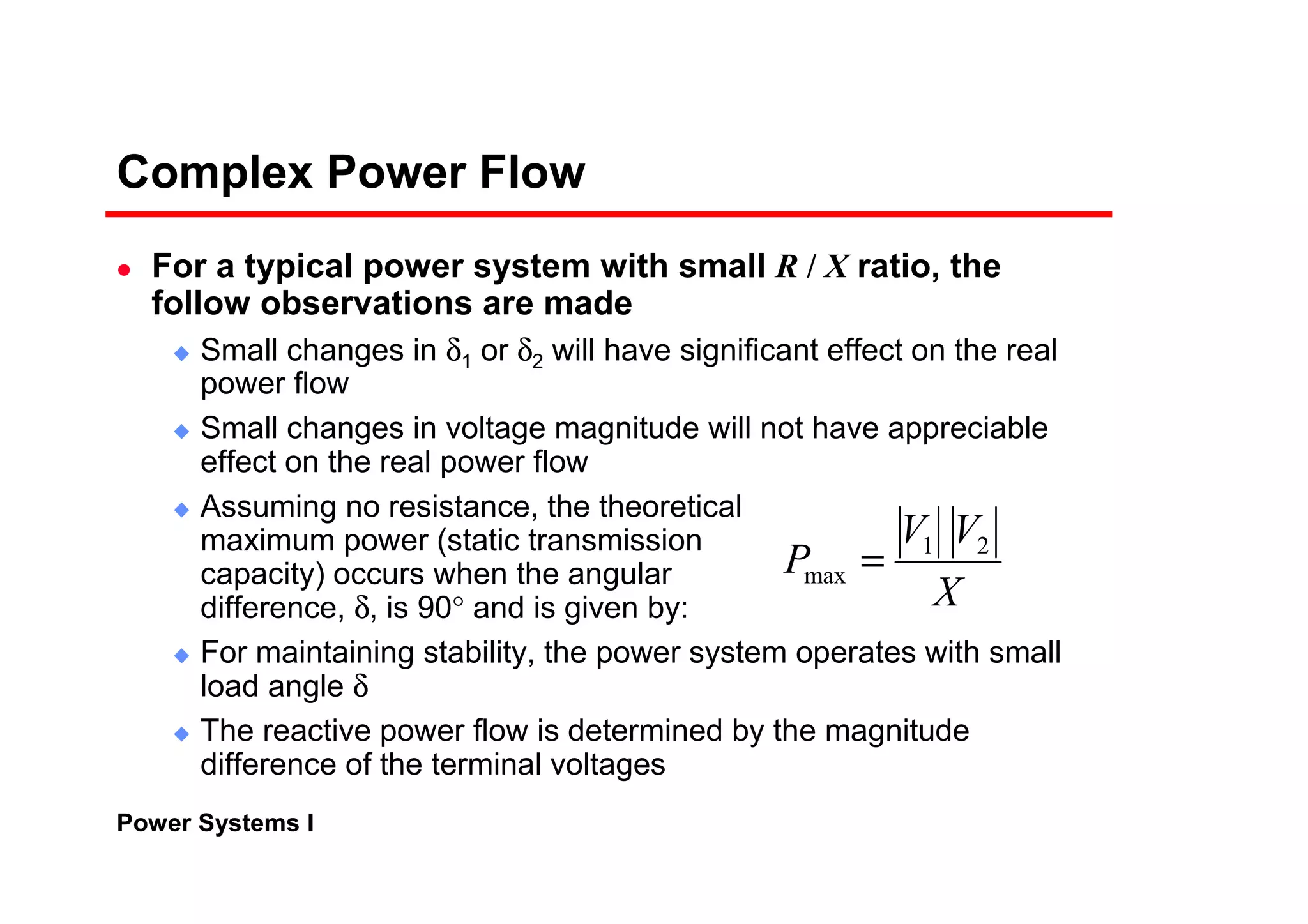
Complex Power Flow
The real and reactive power at the sending end
Transmission lines have small resistance compared to the
reactance. Often, it is assumed R = 0 (Z = X∠90°)
( )
( )21
21
2
1
12
21
21
2
1
12
sinsin
coscos
δδγγ
δδγγ
−+−=
−+−=
Z
VV
Z
V
Q
Z
VV
Z
V
P
( ) ( )[ ]2121
1
1221
21
12 cossin δδδδ −−=−= VV
X
V
Q
X
VV
P](https://image.slidesharecdn.com/lecture1-151012073821-lva1-app6891/75/Lecture1-17-2048.jpg)


![Chapter 02 Fundamentals PS [Autosaved].ppt](https://cdn.slidesharecdn.com/ss_thumbnails/chapter02fundamentalsautosaved-240423133722-632ad8f0-thumbnail.jpg?width=640&height=640&fit=bounds)