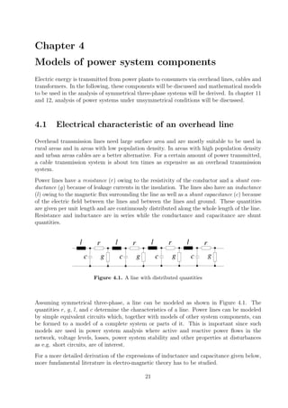
This document discusses the development and structure of the Swedish power system. It began with hydroelectric power stations and later added coal and nuclear power plants. A 220-400kV transmission system was developed to transmit power from northern hydroelectric sources to industrial areas in the south and middle of Sweden. Today the system includes high voltage transmission lines, transformers and substations connecting large centralized power plants ranging from 1000MW to individual consumer needs of kW. The main sources of electricity in Sweden are now hydroelectric, nuclear and some combined heat and power, with hydro and nuclear providing most generation.


![Chapter 3
Alternating current circuits
In this chapter, instantaneous and also complex power in an alternating current (AC) circuit
is discussed. Also, the fundamental properties of AC voltage, current and power in a balanced
(or symmetrical)three-phase circuit are presented.
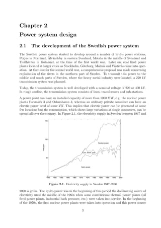
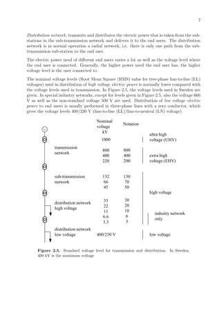
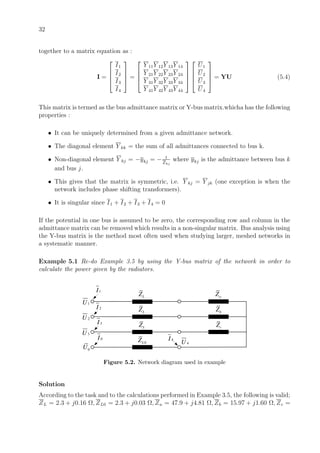
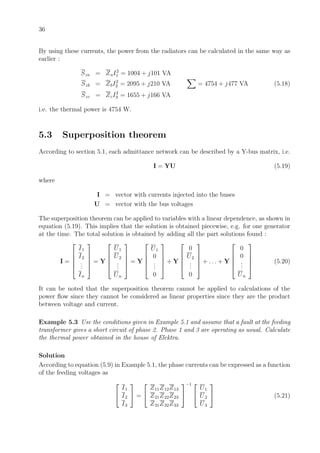
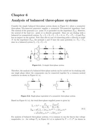
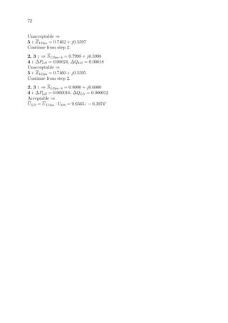
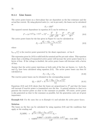
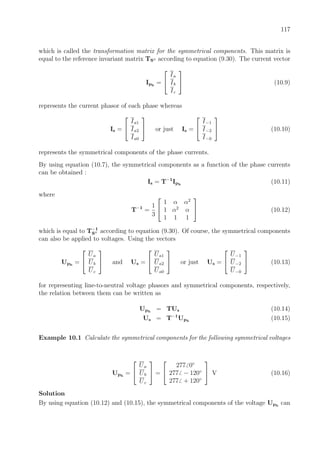
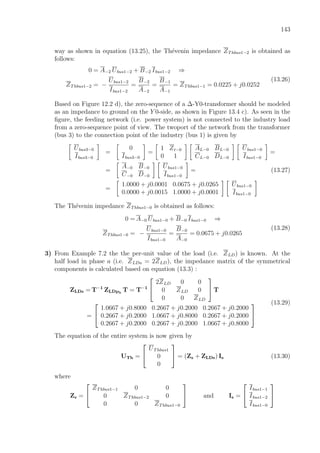
3.1 Single-phase circuit
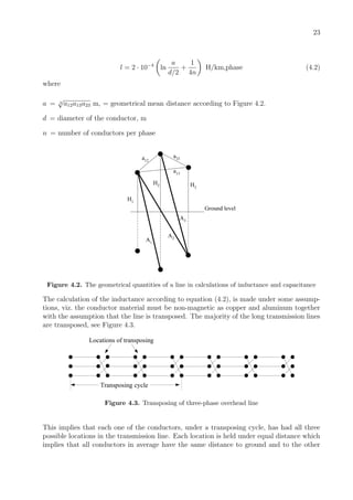
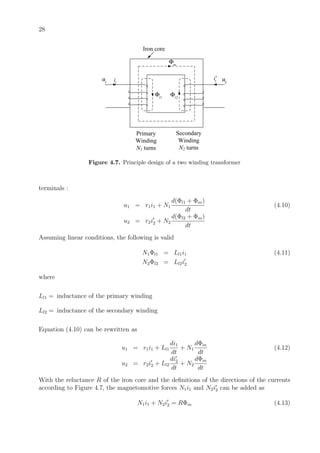
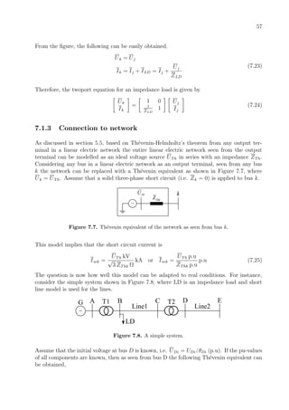
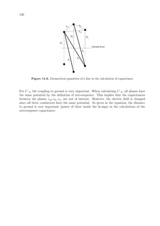
Assume that an AC voltage source with a sinusoidal voltage supplies an impedance load as
shown in Figure 3.1.
Z R jX= +( )u t
( )i t
+
-
Figure 3.1. A sinusoidal voltage source supplies an impedance load.
Let the instantaneous voltage and current be given by
u(t) = UM cos(ωt + θ)
i(t) = IM cos(ωt + γ)
(3.1)
where
UM = the peak value of the voltage
IM =
UM
|Z|
=
UM
Z
= the peak value of the current
ω = 2πf , and f is the frequency of the voltage source
θ = the voltage phase angle
γ = the current phase angle
φ = θ − γ = arctan
X
R
= phase angle between voltage and current
The single-phase instantaneous power consumed by the impedance Z is given by
p(t) = u(t) · i(t) = UM IM cos(ωt + θ) cos(ωt + γ) =
=
1
2
UM IM [cos(θ − γ) + cos(2ωt + θ + γ)] =
=
UM
√
2
IM
√
2
[(1 + cos(2ωt + 2θ)) cos φ + sin(2ωt + 2θ) sin φ] =
= P(1 + cos(2ωt + 2θ)) + Q sin(2ωt + 2θ)
(3.2)
9](https://image.slidesharecdn.com/staticanalysisofpowersystems-150222152940-conversion-gate02/85/Static-analysis-of-power-systems-15-320.jpg)
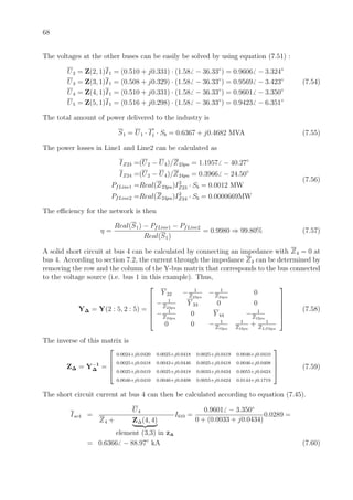
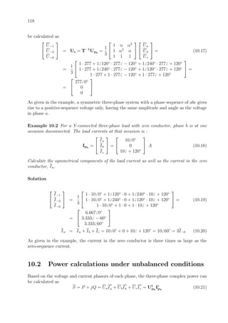
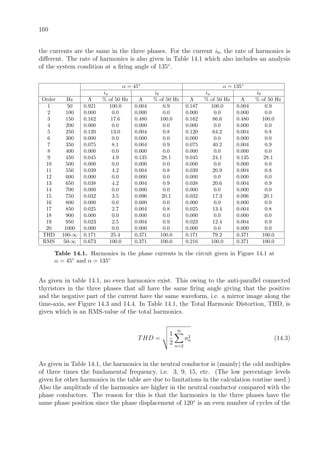
![15
is given by
uab(t) = ua(t) − ub(t) = UM cos(ωt + θ) − UM cos(ωt + θ −
2π
3
) = (3.12)
=
√
3 UM cos(ωt + θ +
π
6
)
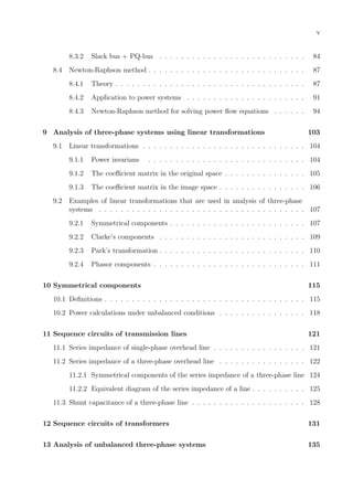
As shown in equation (3.12), in a balanced three-phase circuit the line-to-line voltage leads
the line-to-neutral voltage by 30◦
, and is
√
3 times larger in amplitude (or magnitude, see
equation (3.5)). For instance, at a three-phase power outlet the magnitude of a phase is 230
V, but the magnitude of a line-to-line voltage is
√
3 · 230 = 400 V, i.e. ULL =
√
3 ULN . The
line-to-line voltage uab is shown at the bottom of Figure 3.6.
Next, assume that the voltages given in equation (3.11) supply a balanced (or symmetrical)
three-phase load whose phase currents are
ia(t) = IM cos(ωt + γ)
ib(t) = IM cos(ωt + γ −
2π
3
) (3.13)
ic(t) = IM cos(ωt + γ +
2π
3
)
Then, the total instantaneous power is given by
p3(t) = pa(t) + pb(t) + pc(t) = ua(t)ia(t) + ub(t)ib(t) + uc(t)ic(t) =
=
UM
√
2
IM
√
2
[(1 + cos 2(ωt + θ)) cos φ + sin 2(ωt + θ) sin φ] +
+
UM
√
2
IM
√
2
[(1 + cos 2(ωt + θ −
2π
3
)) cos φ + sin 2(ωt + θ −
2π
3
) sin φ] +
+
UM
√
2
IM
√
2
[(1 + cos 2(ωt + θ +
2π
3
)) cos φ + sin 2(ωt + θ +
2π
3
) sin φ] = (3.14)
= 3
UM
√
2
IM
√
2
cos φ + cos 2(ωt + θ) + cos 2[ωt + θ −
2π
3
] + cos 2[ωt + θ +
2π
3
]
=0
+
+ sin 2(ωt + θ) + sin 2[ωt + θ −
2π
3
] + sin 2[ωt + θ +
2π
3
]
=0
=
= 3
UM
√
2
IM
√
2
cos φ = 3 ULN I cos φ
Note that the total instantaneous power is equal to three times the active power of a single
phase, and it is constant. This is one of the main reasons why three-phase systems have
been used.](https://image.slidesharecdn.com/staticanalysisofpowersystems-150222152940-conversion-gate02/85/Static-analysis-of-power-systems-21-320.jpg)


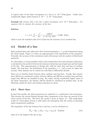
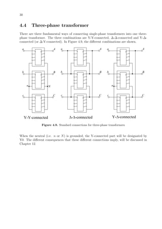

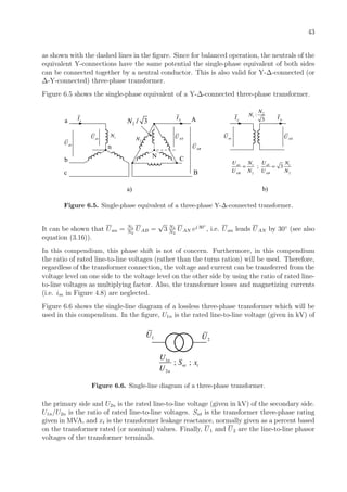
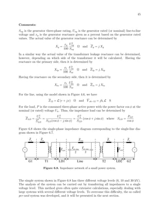
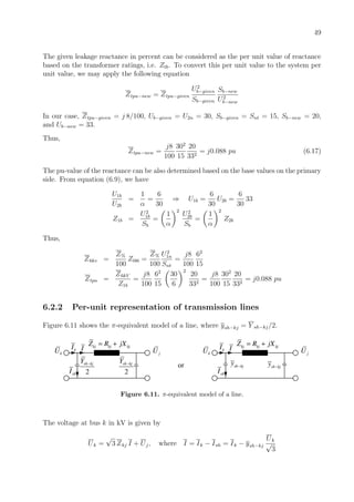
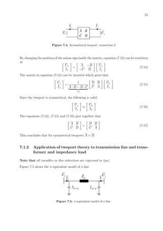
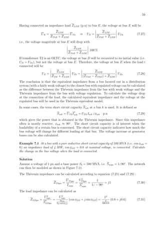
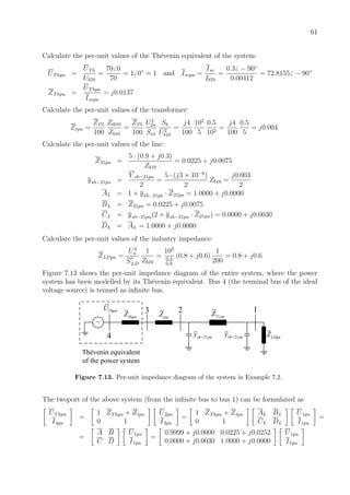
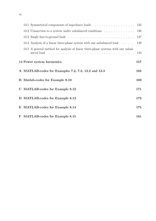
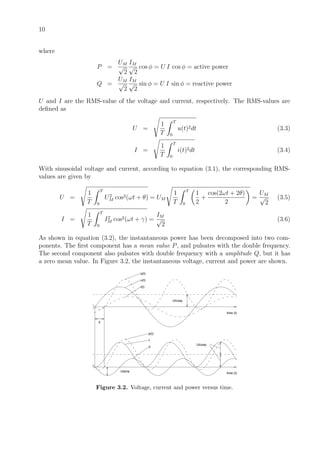
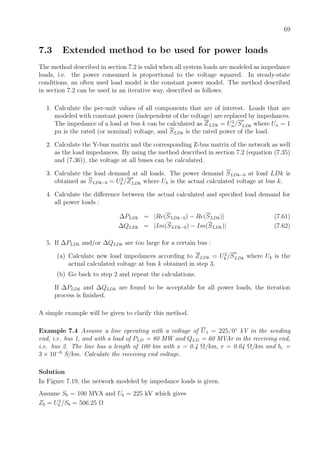
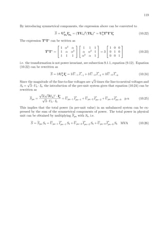
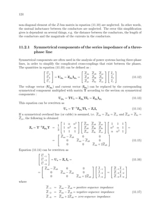
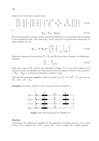
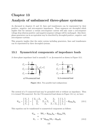
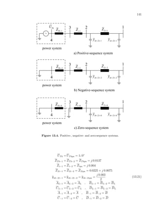
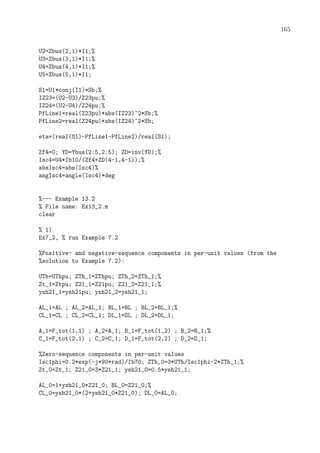
![66
• Transformer T1 : 800 kVA, 70/10, x = 7 %
• Transformer T2 : 300 kVA, 10/0.4, x = 8 %
• Line1 : r = 0.17 Ω/km, ωL = 0.3Ω/km, ωC = 3.2 × 10⁻⁶
S/km, L = 2 km
• Line2 : r = 0.17 Ω/km, ωL = 0.3Ω/km, ωC = 3.2 × 10⁻⁶
S/km, L = 1 km
• Load LD1 : impedance load, 500 kW, cosφ = 0.80, inductive at 10 kV
• Load LD2 : impedance load, 200 kW, cosφ = 0.95, inductive at 0.4 kV
The π-equivalent model is used for the lines.
Calculate the efficiency of the internal network as well as the short circuit current that is
obtained at a solid three-phase short circuit at bus 4.
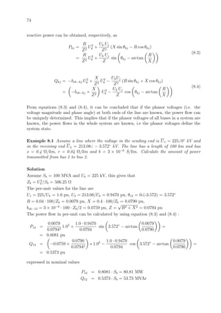
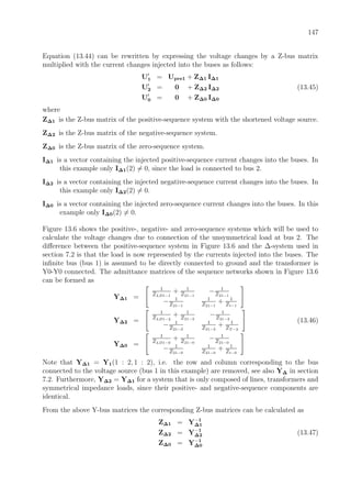
Solution
Chose base values (MVA, kV, ⇒ kA, Ω) : Sb = 500 kVA = 0.5 MVA, Ub70 = 70 kV
1
2 3
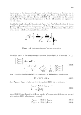
4 5
1t puZ
23 puZ
23sh puy − 1LD puZ
24 puZ
2LD puZ
2t puZ
24sh puy −
Figure 7.18. Network in Example 7.3.
Ub10 = 10 kV ⇒ Ib10 = Sb/
√
3Ub10 = 0.0289 kA, Zb10 = U2
b10/Sb = 200 Ω
Ub04 = 0.4 kV ⇒ Ib04 = Sb/
√
3Ub04 = 0.7217 kA, Zb04 = U2
b04/Sb = 0.32 Ω
Calculate the per-unit values of the infinite bus :
U1 = 70/Ub70 = 70/70 = 1
Calculate the per-unit values of the transformer T1 :
Zt1pu = (Zt1%/100) · Zt1b10/Zb10 = (ZT1%/100) · Sb/Snt1 = (j7/100) · 0.5/0.8 = j0.0438
Calculate the per-unit values of the transformer T2 :
Zt2pu = (Zt2%/100) · Sb/Snt2 = (j8/100) · 0.5/0.3 = j0.1333
Calculate the per-unit values of Line1 :
Z23pu = 2 · [0.17 + j0.3]/Zb10 = 0.0017 + j0.003
ysh−23pu = Y sh−23pu/2 = 2 · [3.2 × 10−6
] · Zb10/2 = j0.0013/2](https://image.slidesharecdn.com/staticanalysisofpowersystems-150222152940-conversion-gate02/85/Static-analysis-of-power-systems-72-320.jpg)
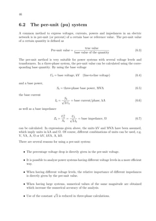
![67
Calculate the per-unit values of Line2 :
Z24pu = 1 · [0.17 + j0.3]/Zb10 = 0.0009 + j0.0015
ysh−24pu = Y sh−24pu/2 = 1 · [3.2 × 10−6
] · Zb10/2 = j0.00064/2
Calculate the per-unit values of the impedance LD1 :
ZLD1pu = (U2
LD1/S
∗
LD1)/Zb10 = (102
/[0.5/0.8]) · (0.8 + j0.6)/200 = 0.64 + j0.48
Calculate the per-unit values of the impedance LD2 :
ZLD2pu = (U2
LD2/S
∗
LD2)/Zb04 = (0.42
/0.2/0.95)·(0.95+j
√
1 − 0.952)/0.32 = 2.2562+j0.7416
Calculate the Y-bus matrix of the network. The grounding point is not included in the Y-bus
matrix since the system then is overdetermined.
Y =
1
Zt1pu
− 1
Zt1pu
0 0 0
− 1
Zt1pu
Y 22 − 1
Z23pu
− 1
Z24pu
0
0 − 1
Z23pu
Y 33 0 0
0 − 1
Z24pu
0 Y 44 − 1
Zt2pu
0 0 0 − 1
Zt2pu
1
Zt2pu
+ 1
ZLD2pu
(7.49)
where
Y 22 =
1
Zt1pu
+
1
Z23pu
+ ysh−23pu +
1
Z24pu
+ ysh−24pu
Y 33 =
1
Z23pu
+ ysh−23pu +
1
ZLD1pu
Y 44 =
1
Z24pu
+ ysh−24pu +
1
Zt2pu
Next, we have
I = YU (7.50)
which can be rewritten as
U1
U2
U3
U4
U5
= U = Y−1
I = ZI = Z
I1
I2
I3
I4
I5
(7.51)
The Z-bus matrix can be calculated by inverting the Y-bus matrix :
Z =
0.510+j0.375 0.510+j0.331 0.508+j0.329 0.510+j0.331 0.516+j0.298
0.510+j0.331 0.510+j0.331 0.508+j0.329 0.510+j0.331 0.516+j0.298
0.508+j0.329 0.508+j0.329 0.509+j0.330 0.508+j0.329 0.515+j0.296
0.510+j0.331 0.510+j0.331 0.508+j0.329 0.510+j0.332 0.517+j0.299
0.516+j0.298 0.516+j0.298 0.515+j0.296 0.517+j0.299 0.529+j0.397
(7.52)
Since all injected currents with exception of I1 are zero, I1 can be calculated using the first
row in equation (7.51) :
U1 = Z(1, 1)I1 ⇒ I1 = U1/Z(1, 1) = 1.0/(0.510 + j0.375) = 1.58 − 36.33◦
(7.53)](https://image.slidesharecdn.com/staticanalysisofpowersystems-150222152940-conversion-gate02/85/Static-analysis-of-power-systems-73-320.jpg)
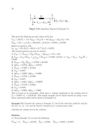
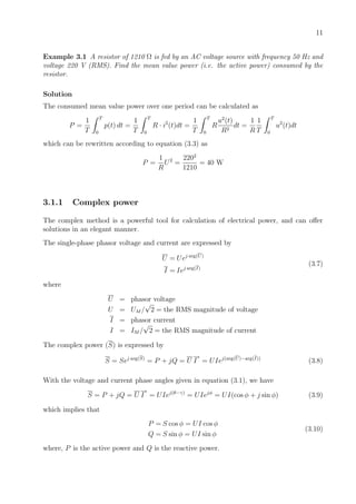
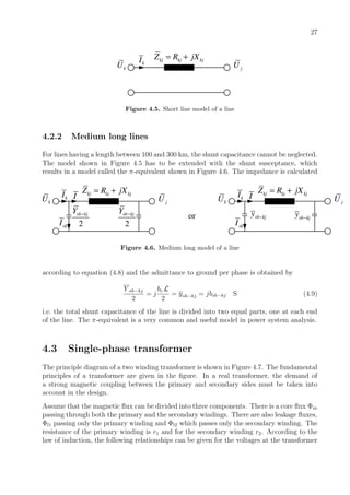
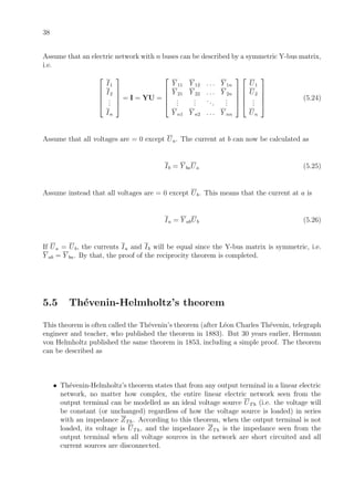
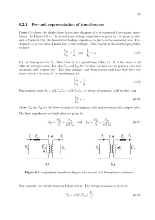
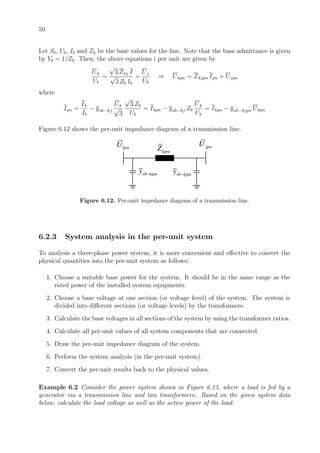
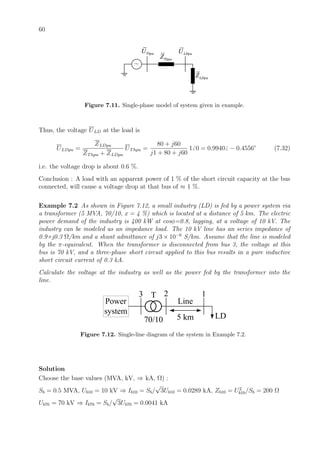
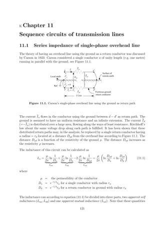
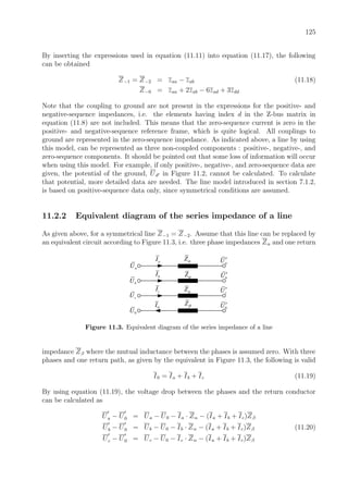
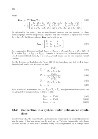
![71
totpuZ
ThpuU
LD LD LDS P jQ= +
LDpuU
Figure 7.20. Network used in Example 7.5.
The total impedance between bus 1 and bus 4 is given by:
Ztotpu = ZThpu + Ztpu + Z21pu = 0.0225 + j0.0252
Calculate the per-unit values of the power demand of the industry as well as the correspond-
ing impedance at nominal voltage :
SLDpu = (PLD + j[PLD/ cos φ] · sin φ)/Sb = 0.8000 + j0.6000
ZLDpu = (U2
n/S
∗
LDpu)/U2
b10 = 0.8 + j0.6
2 : The Y-bus matrix of the network can be calculated as :
Y =
1
Ztotpu
− 1
Ztotpu
− 1
Ztotpu
1
Ztotpu
+ 1
ZLDpu
=
19.67 − j22.08 −19.67 + j22.08
−19.67 + j22.08 20.47 − j22.68
(7.63)
The Z-bus matrix is calculated as the inverse of the Y-bus matrix :
Z = Y−1
=
0.82 + j0.63 0.80 + j0.60
0.80 + j0.60 0.80 + j0.60
(7.64)
The voltage at the industry is now calculated according to equation (7.36) :
ULDpu = Z(2, 1) · UThpu/Z(1, 1) = 0.9679 − 0.3714◦
(7.65)
3 : The power delivered to the industry can be calculated as :
SLDpu−b = U2
LD/Z
∗
LDpu = 0.7495 + j0.5621 (7.66)
4 : The difference between calculated and specified power can be calculated as :
∆PLD = |Re(SLDpu−b) − Re(SLDpu)| = 0.0505 (7.67)
∆QLD = |Im(SLDpu−b) − Im(SLDpu)| = 0.0379 (7.68)
5 : These deviations are too large and the calculations are therefore repeated and a new
industry impedance is calculated by using the new voltage magnitude :
ZLDpu = (U2
LDpu/S
∗
LDpu) = 0.7495 + j0.5621 (7.69)
Repeat the calculations from step 2.
2, 3 : ⇒ SLDpu−b = 0.7965 + j0.5974
4 : ∆PLD = 0.0035, ∆QLD = 0.0026](https://image.slidesharecdn.com/staticanalysisofpowersystems-150222152940-conversion-gate02/85/Static-analysis-of-power-systems-77-320.jpg)
![77
The losses can also be calculated by using the receiving end conditions
Pf (MW) = R
P2
21 + (Q21 + bsh−12U2
2 )2
U2
2
Sb =
= 0.0079
(−0.80)2
+ (−0.60 + 0.0759 · 0.94702
)2
0.94702
100 = 0.81 MW
or by using equation (8.10)
Pf (MW) = [P12 + P21]Sb = [0.8081 + (−0.80)]100 = 0.81 MW
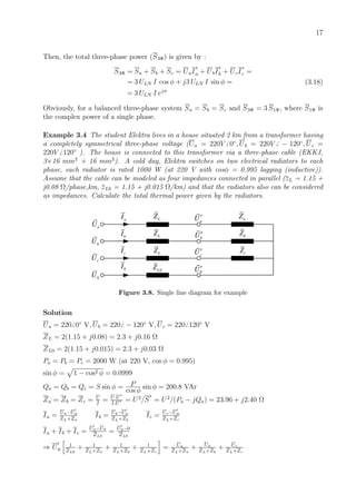
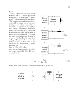
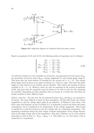
8.1.2 Shunt capacitors and shunt reactors
As mentioned earlier in subsection 8.1.1, transmission of reactive power will increase the
line losses. An often used solution is to generate reactive power as close to the load as
possible. This is done by switching in shunt capacitors. Figure 8.2 shows a Y-connected
shunt capacitor. Figure 8.2 also shows the single-phase equivalent which can be used at
phase a
c
Three-phase connection Single-phase equivalent
phase b
phase c
c
c
c
Figure 8.2. Y -connected shunt capacitors.
symmetrical conditions. A shunt capacitor generates reactive power proportional to the bus
voltage squared U2
. In the per-unit system, we have
Qsh = BshU2
= 2πfc U2
(8.12)
An injection of reactive power into a certain bus will increase the bus voltage, see Example
8.6. The insertion of shunt capacitors in the network is also called phase compensation. This
because the phase displacement between voltage and current is reduced when the reactive
power transmission through the line is reduced.
As mentioned earlier, lines that are lightly loaded generates reactive power. The amount of
reactive power generated is proportional to the length of the line. In such situations, the
reactive power generation will be too large and it is necessary to consume the reactive power
in order to avoid overvoltages. One possible countermeasure is to connect shunt reactors.
They are connected and modeled in the same way as the shunt capacitors with the difference
that the reactors consume reactive power.](https://image.slidesharecdn.com/staticanalysisofpowersystems-150222152940-conversion-gate02/85/Static-analysis-of-power-systems-83-320.jpg)
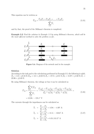
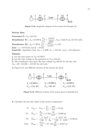
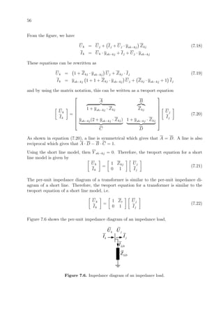
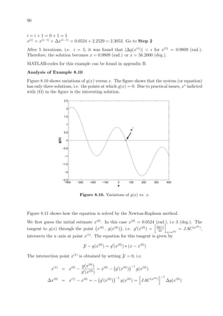
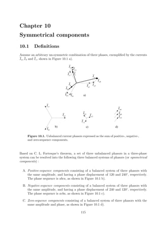
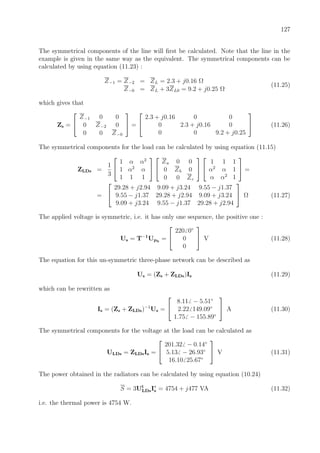
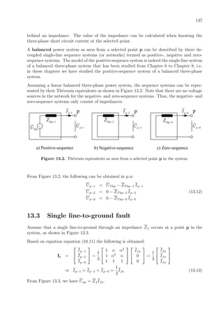
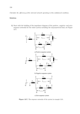
![85
Example 8.6 Use the data given in Example 8.5 with PD2 = 80 MW and QD2 ≈ 60 MVAr.
Use these load levels as a base case and calculate the voltage U2 when the active and reactive
load demand are varying between 0–100 MW and 0–100 MVAr, respectively.
Solution
By using equations (8.23) and (8.24), the voltage can be calculated. The result is shown in
Figure 8.7. The base case, i.e. PD2 = 80 MW and QD2 = 60 MVAr, is marked by circles on
0 10 20 30 40 50 60 70 80 90 100
200
205
210
215
220
225
QD2=60 MVAr, PD2=0-100 MW
PD2=80 MW, QD2=0-100 MVAr
MW or MVAr
U2[kV]
Figure 8.7. The voltage U2 as a function of PD2 and QD2
both curves. As shown in the figure, the voltage drops at bus 2 as the load demand increases.
The voltage at bus 2 is much more sensitive to a change in reactive load demand compared
to a change in active demand. If a shunt capacitor generating 10 MVAr is connected at
bus 2 when having a reactive load demand of 60 MVAr, the net demand of reactive power
will decrease to 50 MVAr and the bus voltage will increase by two kV, from 213 kV to 215
kV. As discussed earlier in subsection 8.1.1, a reduced reactive power load demand will also
reduce the losses on the line.
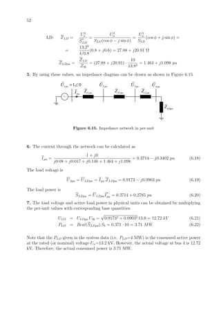
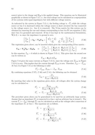
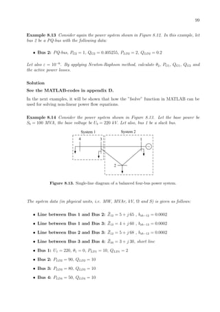
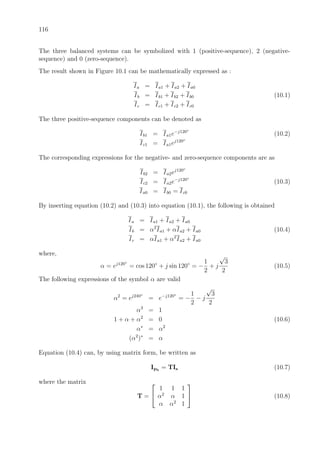
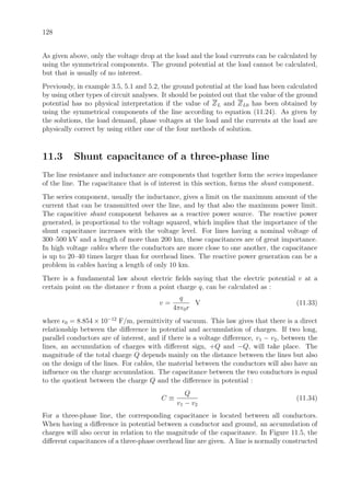
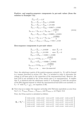
Example 8.7 Use the base case in Example 8.6, i.e. PD2 = 80 MW and QD2 = 60 MVAr.
Calculate the voltage U2 when the series compensation of the line is varied in the interval
0–100 %.
Solution
A series compensation of 0–100 % means that 0–100 % of the line reactance is compensated
by series capacitors. 0 % means no series compensation at all and 100 % means that Xc = X.
The voltage can be calculated by using equations (8.23) and (8.24). The result is shown in
Figure 8.8. As shown in Figure 8.8, the voltage at bus 2 increases as the degree of series
compensation increases. If the degree of compensation is 40 %, the voltage at bus 2 is
increased by 4.5 kV (= 2 %) from 213.1 kV to 217.6 kV.
When having short lines or when only interested in approximate calculations, the shunt
capacitance of a line can be neglected. In these conditions, bsh−21 in equation (8.23) is](https://image.slidesharecdn.com/staticanalysisofpowersystems-150222152940-conversion-gate02/85/Static-analysis-of-power-systems-91-320.jpg)
![86
0 10 20 30 40 50 60 70 80 90 100
210
215
220
225
% compensation
U2[kV]
Figure 8.8. The voltage U2 as a function of degree of compensation
neglected, and the equation will be rewritten as
U2 =
U2
1 − 2a1
2
+
(−)
U2
1 − 2a1
2
2
− (a2
1 + a2
2) (8.25)
where
a1 = −R P21 − X Q21
a2 = −X P21 + R Q21
Example 8.8 Use the data given in Example 8.5. Calculate the magnitude of the voltage
by using the approximate expression given by equation (8.25).
Solution
Equation (8.25) gives that
a1 = −0.0790(−0.8) + 0.0079(−0.6) = 0.0537
a2 = 0.0079(−0.6) − 0.0790(−0.8) = 0.0585
⇒
U2 = 0.9410
⇒
U2(kV) = 0.9410 · Sb = 211.72 kV
i.e. the voltage becomes 0.6 % too low compared to the more accurate result.
Another approximation often used, is to neglect a2 in equation (8.25). That equation can
then be rewritten as
U2 ≈
U1
2
+
U2
1
4
+ R P21 + X Q21 (8.26)](https://image.slidesharecdn.com/staticanalysisofpowersystems-150222152940-conversion-gate02/85/Static-analysis-of-power-systems-92-320.jpg)
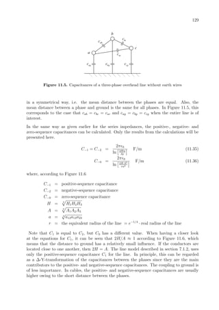
![89
Yes
No
( )
Give i
x
Set 0i =
( )i
x x=
Step 1
Step 2
Step Final
( )
Calculate ( )i
g x∆
( )
Is the magnitude of the all entries of ( )
less than a small positve number
?
i
g x∆
( ) ( 1) ( 1)
1
i i i
i i
x x x− −
= +
= + ∆
Step 3
Step 4( )
Calculate i
x∆
Step 5
( )
Calculate i
JAC
Figure 8.9. Flowchart for the Newton-Raphson method.
Example 8.10 Using the Newton-Raphson method, solve for x of the equation
g(x) = k1 x + k2 cos(x − k3) − k4 = 0
Let k1 = −0.2, k2 = 1.2, k3 = −0.07, k4 = 0.4 and = 10−4
. (This equation is used in the
assignment D1.)
Solution
This equation is of the form given by (8.28), with f(x) = k1 x + k2 cos(x − k3) and b = k4.
Step 1
Set i = 0 and x(i)
= x(0)
= 0.0524 (radians), i.e. 3 (degrees).
Step 2
∆g(x(i)
) = b − f(x(i)
) = 0.4 − [(−0.2 ∗ 0.0524) + 1.2 cos(0.0524 + 0.07)] = −0.7806
Go to Step 3 since |∆g(x(i)
)| >
Step 3
JAC(x(i))
= ∂f
∂x x=x(i) = −0.2 − 1.2 sin(0.0524 + 0.07) = −0.3465
Step 4
∆x(i)
= JAC(x(i))
−1
∆g(x(i)
) = −0.7806
−0.3465
= 2.2529
Step 5](https://image.slidesharecdn.com/staticanalysisofpowersystems-150222152940-conversion-gate02/85/Static-analysis-of-power-systems-95-320.jpg)
![91
0
g(x)
x
(0)
x(1)
x
(2)
g(x
(0)
)
JAC(x
(0)
)
g(x(1)
)
JAC(x
(1)
)
Figure 8.11. Variations of g(x) vs. x.
In a similar manner, x(2)
can be obtained which is hopefully a better estimate than x(1)
. As
shown in the figure, from x(2)
we obtain x(3)
which is a better estimate of x∗
than what x(2)
does. This iterative method will be continued until |∆g(x)| < .
Example 8.11 Solve for x in Example 8.10, but let x(0)
= 0.0174 (rad.), i.e. 1 (deg.).
Solution
D.I.Y, (i.e., Do It Yourself)
8.4.2 Application to power systems
Consider a power system with N buses. The aim is to determine the voltage at all buses
in the system by applying the Newton-Raphson method. All variables are expressed in
pu.
Consider again Figure 8.1. Let
gkj + j bkj =
1
Zkj
=
1
R + j X
=
R
Z2
+ j
−X
Z2
⇒
gkj =
R
Z2
bkj = −
X
Z2
(8.37)
Based on (8.37), we rewrite (8.3) and (8.4) as follows
Pkj = gkj U2
k − Uk Uj [gkj cos(θkj) + bkj sin(θkj)] (8.38)
Qkj = U2
k (−bsh−kj − bkj) − Uk Uj [gkj sin(θkj) − bkj cos(θkj)] (8.39)](https://image.slidesharecdn.com/staticanalysisofpowersystems-150222152940-conversion-gate02/85/Static-analysis-of-power-systems-97-320.jpg)
![92
The current through the line, and the loss in the line can be calculated by
Ikj =
Pkj − j Qkj
U
∗
k
(8.40)
Plkj = Pkj + Pjk (8.41)
Qlkj = Qkj + Qjk (8.42)
Consider again Figure 8.4. Let Y = G + jB denote the admittance matrix of the system (or
Y-matrix), where Y is an N × N matrix, i.e. the system has N buses. The relation between
the injected currents into the buses and the voltages at the buses is given by I = Y U, see
section 5.1. Therefore, the injected current into bus k is given by Ik = N
j=1 Y kj Uj.
The injected complex power into bus k can now be calculated by
Sk = Uk I
∗
k = Uk
N
j=1
Y
∗
kjU
∗
j = Uk
N
j=1
(Gkj − jBkj) Uj(cos(θkj) + j sin(θkj))
= Uk
N
j=1
Uj [Gkj cos(θkj) + Bkj sin(θkj)] + j Uk
N
j=1
Uj [Gkj sin(θkj) − Bkj cos(θkj)]
Let Pk denote the real part of Sk, i.e. the injected active power, and Qk denote the imaginary
part of Sk, i.e. the injected reactive power, as follows:
Pk = Uk
N
j=1
Uj [Gkj cos(θkj) + Bkj sin(θkj)]
Qk = Uk
N
j=1
Uj [Gkj sin(θkj) − Bkj cos(θkj)]
(8.43)
Note that Gkj = −gkj and Bkj = −bkj for k = j. Furthermore,
Pk =
N
j=1
Pkj
Qk =
N
j=1
Qkj
Equations (8.18) and (8.19) can now be rewritten as
Pk − PGDk = 0
Qk − QGDk = 0
(8.44)](https://image.slidesharecdn.com/staticanalysisofpowersystems-150222152940-conversion-gate02/85/Static-analysis-of-power-systems-98-320.jpg)
![93
which are of the form given in equation (8.28), where
x =
θ
U
=
θ1
...
θN
U1
...
UN
, f(θ, U) =
fP (θ, U)
fQ(θ, U)
=
P1
...
PN
Q1
...
QN
, b =
bP
bQ
=
PGD1
...
PGDN
QGD1
...
QGDN
(8.45)
the aim is to determine x = [θ U]T
by applying the Newton-Raphson method.
Assume that there are 1 slack bus and M PU-buses in the system. Therefore, θ becomes an
(N − 1) × 1 vector and U becomes an (N − 1 − M) × 1 vector, why?
Based on (8.34), we define the following:
∆Pk = PGDk − Pk k = slack bus
∆Qk = QGDk − Qk k = slack bus and PU-bus
(8.46)
Based on (8.35), the jacobian matrix is given by
JAC =
∂fP (θ,U)
∂θ
∂fP (θ,U)
∂U
∂fQ(θ,U)
∂θ
∂fQ(θ,U)
∂U
=
H N
J L
(8.47)
where,
H is an (N − 1) × (N − 1) matrix
N is an (N − 1) × (N − M − 1) matrix
J is an (N − M − 1) × (N − 1) matrix
L is an (N − M − 1) × (N − M − 1) matrix
The entries of these matrices are given by:
Hkj = ∂Pk
∂θj
k = slack bus j = slack bus
Nkj = ∂Pk
∂Uj
k = slack bus j = slack bus and PU-bus
Jkj = ∂Qk
∂θj
k = slack bus and PU-bus j = slack bus
Lkj = ∂Qk
∂Uj
k = slack bus and PU-bus j = slack bus and PU-bus
Based on (8.32), (8.46) and (8.47), the following is obtained
H N
J L
∆θ
∆U
=
∆P
∆Q
(8.48)
To simplify the entries of the matrices N and L , these matrices are multiplied with U.
Then, (8.48) can be rewritten as
H N
J L
∆θ
∆U
U
=
∆P
∆Q
(8.49)](https://image.slidesharecdn.com/staticanalysisofpowersystems-150222152940-conversion-gate02/85/Static-analysis-of-power-systems-99-320.jpg)
![94
where,
for k = j
Hkj = ∂Pk
∂θj
= Uk Uj [Gkj sin(θkj) − Bkj cos(θkj)]
Nkj = Uj Nkj = Uj
∂Pk
∂Uj
= Uk Uj [Gkj cos(θkj) + Bkj sin(θkj)]
Jkj = ∂Qk
∂θj
= −Uk Uj [Gkj cos(θkj) + Bkj sin(θkj)]
Lkj = Uj Lkj = Uj
∂Qk
∂Uj
= Uk Uj [Gkj sin(θkj) − Bkj cos(θkj)]
(8.50)
and for k = j
Hkk = ∂Pk
∂θk
= −Qk − BkkU2
k
Nkk = Uk
∂Pk
∂Uk
= Pk + GkkU2
k
Jkk = ∂Qk
∂θk
= Pk − GkkU2
k
Lkj = Uk
∂Qk
∂Uk
= Qk − BkkU2
k
(8.51)
Now based on (8.36), the following is obtained:
∆θ
∆U
U
=
H N
J L
−1
∆P
∆Q
(8.52)
Finally, U and θ will be updated as follows:
θk = θk + ∆θk k = slack bus
Uk = Uk 1 + ∆Uk
Uk
k = slack bus and PU-bus
(8.53)
8.4.3 Newton-Raphson method for solving power flow equations
Newton-Raphson method can be applied to non-linear power flow equations as follows:
• Step 1
1a) Read bus and line data. Identify slack bus (i.e. Uθ-bus), PU-buses and PQ-buses.
1b) Develop the Y-matrix and calculate the net productions, i.e. PGD = PG − PLD
and QGD = QG − QLD.
1c) Give the initial estimate of the unknown variables, i.e. U for PQ-buses and θ for
PU- and PQ-buses. It is very common to set U = Uslack and θ = θslack. However,
the flat initial estimate may also be applied, i.e. U = 1 and θ = 0.
1d) Go to Step 2.
• Step 2](https://image.slidesharecdn.com/staticanalysisofpowersystems-150222152940-conversion-gate02/85/Static-analysis-of-power-systems-100-320.jpg)
![95
2a) Calculate the injected power into each bus by equation (8.43).
2b) Calculate the difference between the net production and the injected power for
each bus, i.e. ∆P and ∆Q by equation (8.46).
2c) Is the magnitude of all entries of [∆P ∆Q]T
less than a specified small positive
constant ?
∗ If yes, go to Step Final.
∗ if no, go to Step 3.
• Step 3
3a) Calculate the jacobian by equations (8.50) and (8.51).
3b) Go to Step 4.
• Step 4
4a) Calculate ∆θ ∆U
U
T
by equation (8.52).
4b) Go to Step 5.
• Step 5
5a) Update U and θ by equation (8.53).
5b) Go till Step 2.
• Step Final
– Calculate the generated powers, i.e. PG (MW) and QG (MVAr) in the slack bus,
and QG (MVAr) in the PU-buses by using equation (8.44).
– Calculate the power flows (MW, MVAr) by using equations (8.38) and (8.39).
– Calculate active power losses (MW) by using equation (8.41).
– Give all the voltage magnitudes (kV) and the voltage phase angles (degrees).
– Print out the results.
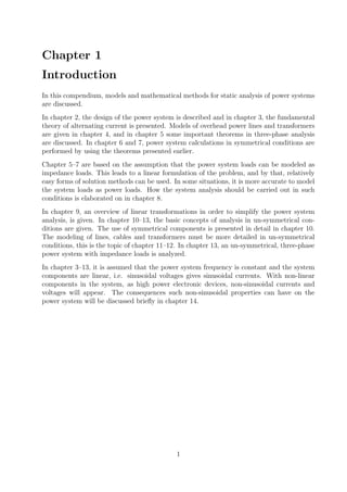
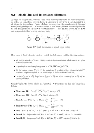
Example 8.12 Consider the power system shown in Figure 8.12. Let Sb = 100 MVA, and
Ub = 220 kV.
1 2
~ ~
Figure 8.12. Single-line diagram of a balanced two-bus power system.
The following data (all in pu) is known:](https://image.slidesharecdn.com/staticanalysisofpowersystems-150222152940-conversion-gate02/85/Static-analysis-of-power-systems-101-320.jpg)
![96
• Line between Bus 1 and Bus 2: short line, ¯Z12 = 0.02 + j 0.2
• Bus 1: slack bus, U1 = 1, θ1 = 0, PLD1 = 0.2, QLD1 = 0.02
• Bus 2: PU-bus, U2 = 1, PG2 = 1, PLD2 = 2, QLD2 = 0.2
By applying Newton-Raphson method, calculate θ2, PG1, QG1, QG2 and the active power
losses in the system after 3 iterations.
Solution
MATLAB-codes for this example can be found in appendix C.
Step 1
1a) bus 1 is a slack bus , bus 2 is a PU-bus , U1 = 1, U2 = 1, θ1 = 0.
1b)
Y =
1
¯Z12
− 1
¯Z12
− 1
¯Z12
1
¯Z12
=
G11 + j B11 G12 + j B12
G21 + j B21 G22 + j B22
=
=
0.4950 − j 4.9505 −0.4950 + j 4.9505
−0.4950 + j 4.9505 0.4950 − j 4.9505
= G + j B
PGD2 = PG2 − PLD2 = 1 − 2 = −1
No QGD since there is no PQ-bus in the system.
1c)
Since the system has only one slack bus and one PU-bus, the phase angle of the PU-bus is
the only unknown variable. As an initial value , let θ2 = 0.
Iteration 1
Step 2
2a)
P2 = U2 U1 [G21 cos(θ2 − θ1) + B21 sin(θ2 − θ1)] + U2
2 G22 =
= 1 ∗ 1 ∗ [−0.4950 ∗ cos(0 − 0) + 4.9505 ∗ sin(0 − 0)] + 12
∗ 0.4950 = 0
2b)
∆P = ∆P2 = PGD2 − P2 = −1 − 0 = −1
Step 3
Q2 = U2 U1 [G21 sin(θ2 − θ1) − B21 cos(θ2 − θ1)] − U2
2 B22 =
= 1 ∗ 1 ∗ [−0.4950 ∗ sin(0 − 0) − 4.9505 ∗ cos(0 − 0)] − 12
∗ (−4.9505) = 0
H =
∂P2
∂θ2
= −Q2 − B22U2
2 = −0 − (−4.9505 ∗ 12
) = 4.9505
JAC = H = 4.9505](https://image.slidesharecdn.com/staticanalysisofpowersystems-150222152940-conversion-gate02/85/Static-analysis-of-power-systems-102-320.jpg)
![97
Step 4
∆θ2 = H−1
∆P2 =
−1
4.9505
= −0.2020
Step 5
θ2 = θ2 + ∆θ2 = 0 − 0.2020 = −0.2020
Iteration 2
Step 2
2a)
P2 = U2 U1 [G21 cos(θ2 − θ1) + B21 sin(θ2 − θ1)] + U2
2 G22 =
= 1 ∗ 1 ∗ [−0.4950 ∗ cos(−0.2020 − 0) + 4.9505 ∗ sin(−0.2020 − 0)] + 12
∗ 0.4950 = −0.9831
2b)
∆P = ∆P2 = PGD2 − P2 = −1 − (−0.9831) = −0.0169
Step 3
Q2 = U2 U1 [G21 sin(θ2 − θ1) − B21 cos(θ2 − θ1)] − U2
2 B22 =
= 1 ∗ 1 ∗ [−0.4950 ∗ sin(−0.2020 − 0) − 4.9505 ∗ cos(−0.2020 − 0)] − 12
∗ (−4.9505) = 0.2000
H =
∂P2
∂θ2
= −Q2 − B22U2
2 = −0.2000 − (−4.9505 ∗ 12
) = 4.7505
JAC = H = 4.7505
Step 4
∆θ2 = H−1
∆P2 =
−0.0169
4.7505
= −0.0035
Step 5
θ2 = θ2 + ∆θ2 = −0.2020 − 0.0035 = −0.2055
Iteration 3
Step 2
2a)
P2 = U2 U1 [G21 cos(θ2 − θ1) + B21 sin(θ2 − θ1)] + U2
2 G22 =
= 1 ∗ 1 ∗ [−0.4950 ∗ cos(−0.2055 − 0) + 4.9505 ∗ sin(−0.2055 − 0)] + 12
∗ 0.4950 = −1.0000
2b)
∆P = ∆P2 = PGD2 − P2 = −1 − (−1.0000) ≈ 0 (in MATLAB ∆P2 = −9.3368 ∗ 10−6
)
Step 3
Q2 = U2 U1 [G21 sin(θ2 − θ1) − B21 cos(θ2 − θ1)] − U2
2 B22 =
= 1 ∗ 1 ∗ [−0.4950 ∗ sin(−0.2055 − 0) − 4.9505 ∗ cos(−0.2055 − 0)] − 12
∗ (−4.9505) = 0.2053
H =
∂P2
∂θ2
= −Q2 − B22U2
2 = −0.2053 − (−4.9505 ∗ 12
) = 4.7452
JAC = H = 4.7452](https://image.slidesharecdn.com/staticanalysisofpowersystems-150222152940-conversion-gate02/85/Static-analysis-of-power-systems-103-320.jpg)
![98
Step 4
∆θ2 = H−1
∆P2 =
−9.3368 ∗ 10−6
4.7452
= −1.9676 ∗ 10−6
≈ 0
Step 5
θ2 = θ2 + 0 = −0.2055 − 0 = −0.2055
Now go to Step Final
Step Final
P1 = U1 U2 [G12 cos(θ1 − θ2) + B12 sin(θ1 − θ2)] + U2
1 G11 =
= 1 ∗ 1 ∗ [−0.4950 ∗ cos(0 + 0.2055) + 4.9505 ∗ sin(0 + 0.2055)] + 12
∗ 0.4950 = 1.0208
Q1 = U1 U2 [G12 sin(θ1 − θ2) − B12 cos(θ1 − θ2)] − U2
1 B11 =
= 1 ∗ 1 ∗ [−0.4950 ∗ sin(0 + 0.2055) − 4.9505 ∗ cos(0 + 0.2055)] − 12
∗ (−4.9505) = 0.0032
Q2 = U2 U1 [G21 sin(θ2 − θ1) − B21 cos(θ2 − θ1)] − U2
2 B22 =
= 1 ∗ 1 ∗ [−0.4950 ∗ sin(−0.2055 − 0) − 4.9505 ∗ cos(−0.2055 − 0)] − 12
∗ (−4.9505) = 0.2053
PG1 = (P1 + PLD1) ∗ Sb = (1.0208 + 0.2) ∗ 100 = 122.08 MW (in MATLAB PG1=122.0843)
QG1 = (Q1 + QLD1) ∗ Sb = (0.0032 + 0.02) ∗ 100 = 2.32 MVAr (in MATLAB QG1=2.3171)
QG2 = (Q2 + QLD2) ∗ Sb = (0.2053 + 0.2) ∗ 100 = 40.53 MVAr (in MATLAB QG2=40.5255)
g = −G , b = −B and bsh−12 = 0
P12 = g12 U2
1 − U1 U2 [g12 cos(θ1 − θ2) + b12 sin(θ1 − θ2)] ∗ Sb =
= 0.4950 ∗ 12
− 1 ∗ 1 ∗ [0.4950 ∗ cos(0 + 0.2055) − 4.9505 ∗ sin(0 + 0.2055)] ∗ 100 =
= 102.0843 MW
P21 = g21 U2
2 − U2 U1 [g21 cos(θ2 − θ1) + b21 sin(θ2 − θ1)] ∗ Sb =
= 0.4950 ∗ 12
− 1 ∗ 1 ∗ [0.4950 ∗ cos(−0.2055 − 0) − 4.9505 ∗ sin(−0.2055 − 0)] ∗ 100 =
= −100 MW
Q12 = (−bsh−12 − b12)U2
1 − U1 U2 [g12 sin(θ1 − θ2) − b12 cos(θ1 − θ2)] ∗ Sb =
= (−0 + 4.9505) ∗ 12
− 1 ∗ 1 ∗ [0.4950 ∗ sin(0 + 0.2055) + 4.9505 ∗ cos(0 + 0.2055)] ∗ 100 =
= 0.3171 MVAr
Q21 = (−bsh−12 − b21)U2
2 − U2 U1 [g21 sin(θ2 − θ1) − b21 cos(θ2 − θ1)] ∗ Sb =
= (−0 + 4.9505) ∗ 12
− 1 ∗ 1 ∗ [0.4950 ∗ sin(−0.2055 − 0) + 4.9505 ∗ cos(−0.2055 − 0)] ∗ 100
= 20.5255 MVAr
Ptot
Loss = P12 + P21 = 102.0843 − 100 = 2.0843 MW
or
Ptot
Loss = (PG1 + PG2) − (PLD1 + PLD2) = (122.0843 + 100) − (20 + 200) = 2.0843 MW
ANG = [θ1 theta2] ∗
180
π
= [0 − 0.2055] ∗
180
π
= [0 − 11.7771◦
]
VOLT = [U1 U2] ∗ Ub = [1 1] ∗ 220 = [220 220]](https://image.slidesharecdn.com/staticanalysisofpowersystems-150222152940-conversion-gate02/85/Static-analysis-of-power-systems-104-320.jpg)


![149
ULDbusrph
=
ULDbusra
ULDbusrb
ULDbusrc
=
ZLDbusra 0 0
0 ZLDbusrb 0
0 0 ZLDbusrc
ILDbusra
ILDbusrb
ILDbusrc
=
= ZLDbusrph
ILDbusrph
(13.50)
By introducing symmetrical components, this can be converted to
U (r) =
Ubusr−1
Ubusr−2
Ubusr−0
= T−1
ULDbusrph
= T−1
ZLDbusrph
ILDbusrph
=
= T−1
ZLDbusrph
T
=ZLDbusrs
ILDbusrs = −ZLDbusrs I∆(r) (13.51)
Note that ILDbusrs is injected into the load, however I∆(r) is injected into the bus. Therefore,
ILDbusrs = −I∆(r).
Next based on equations (13.49) and (13.51), the current I∆(r) can be expressed by
I∆(r) = − [Z∆(r, r) + ZLDbusrs]−1
Upre(r) (13.52)
These values of the symmetrical components of the current at bus r can then be inserted
into equation (13.45) where the symmetrical components of all voltages can be calculated.
The voltage at bus k can then be calculated as :
U1(k) = Upre1(k) + Z∆1(k, r) I∆1(r)
U2(k) = Z∆2(k, r) I∆2(r) (13.53)
U0(k) = Z∆0(k, r) I∆0(r)
Example 13.3 Consider again the system described in Example 7.3. The following addi-
tional data is also given:
• The infinite bus (i.e. bus 1) has and a grounded zero connection point.
• Transformer T1 is ∆-Y0 connected with Y 0 on the 10 kV-side, and Zn = 0.
• Transformer T2 is Y0-Y0 connected with Zn = 0.
• The zero-sequence impedances of the lines are 3 times the positive-sequence impedances,
and the zero-sequence shunt admittances of the lines are 0.5 times the positive-sequence
shunt admittances.
• The load LD1 is ∆-connected.
• The load LD2 is Y0-connected with Zn = 0. Furthermore, half of the normal load
connected to phase a is disconnected while the other phases are loaded as normal, i.e.
LD2 is an unsymmetrical load.](https://image.slidesharecdn.com/staticanalysisofpowersystems-150222152940-conversion-gate02/85/Static-analysis-of-power-systems-155-320.jpg)
![153
where
Y 22−0 =
1
Zt1−0
+
1
Z23−0
+ ysh−23−0 +
1
Z24−0
+ ysh−24−0
Y 33−0 =
1
Z23−0
+ ysh−23−0
Y 44−0 =
1
Z24−0
+ ysh−24−0 +
1
Zt2−0
Corresponding Z-bus matrix is obtained as the inverse
Z∆0 = Y−1
∆0 =
0.0000+j0.0438 0.0000+j0.0438 0.0000+j0.0438 0.0000+j0.0438
0.0000+j0.0438 0.0051+j0.0528 0.0000+j0.0438 0.0000+j0.0438
0.0000+j0.0438 0.0000+j0.0438 0.0026+j0.0483 0.0026+j0.0483
0.0000+j0.0438 0.0000+j0.0438 0.0026+j0.0483 0.0026+j0.1816
(13.63)
Note that element (4,4) corresponds to bus 5. Thus,
ZThbus5−0 = 0.0026 + j0.1816 (13.64)
Next, since all Th´evenin equivalents as seen from bus 5 are identified, the voltage vector
and impedance matrix expressed in equation (13.49) can now be obtained as follows:
Upre(5) =
UThbus5
0
0
=
0.968 − 2.413◦
0
0
Z∆(5, 5) =
ZThbus5−1 0 0
0 ZThbus5−2 0
0 0 ZThbus5−0
= (13.65)
=
0.0026 + j0.1771 0 0
0 0.0026 + j0.1771 0
0 0 0.0026 + j0.1816
3) Determine the symmetrical components of the unsymmetrical load by using equation
(13.51) and ZLD2pu from the solution to Example 7.3.
ZLDbus5s = T−1
ZLDbus5ph
T = T−1
2ZLD2pu 0 0
0 ZLD2pu 0
0 0 ZLD2pu
T =
=
3.0083 + j0.9888 0.7521 + j0.2472 0.7521 + j0.2472
0.7521 + j0.2472 3.0083 + j0.9888 0.7521 + j0.2472
0.7521 + j0.2472 0.7521 + j0.2472 3.0083 + j0.9888
(13.66)
The symmetrical components of the currents through the load can now be determined
by using equations (13.52) and (13.65).
I∆(5) = − [Z∆(5, 5) + ZLDbus5s]−1
U(5) =
0.3315 155.8442◦
0.0653 − 26.5244◦
0.0653 − 26.6221◦
=
I∆1(5)
I∆2(5)
I∆0(5)
(13.67)](https://image.slidesharecdn.com/staticanalysisofpowersystems-150222152940-conversion-gate02/85/Static-analysis-of-power-systems-159-320.jpg)
![155
By using equation (10.25), the total power flowing through ¯Z23 is given by
SZ23in
= SZ23−1 + SZ23−2 + SZ23−0 = 0.4602 + j0.3461 (13.71)
In a similar manner, the following can also be obtained:
SZ24in
= U1(2)I
∗
Z24−1 + U2(2)I
∗
Z24−2 + U0(2)I
∗
Z24−0 = 0.1489 + j0.0567
SZ23out = U1(3)I
∗
Z23−1 + U2(3)I
∗
Z23−2 + U0(3)I
∗
Z23−0 = 0.4589 + j0.3461
SZ24out = U1(4)I
∗
Z24−1 + U2(4)I
∗
Z24−2 + U0(4)I
∗
Z24−0 = 0.1488 + j0.0567
The efficiency can now be obtained as:
η = 100 ·
Real(SZ23out ) + Real(SZ24out )
Real(SZ23in
) + Real(SZ24in
)
= 99.7911% (13.72)
The efficiency can also be calculated as follows:
Sinj = UTh
UTh − U1(2)
Zt1−1
∗
+ U2(2)
0 − U2(2)
Zt1−2
∗
+ U0(2)
0 − U0(2)
Zt1−0
∗
where, Sinj is the total power injected into the system by the infinite bus. Next, the
total load is calculated as follows:
SLDtot =
|U1(3)|2
ZLD1−1
+
|U2(3)|2
ZLD1−2
+0+U1(5)[−I∆1(5)]∗
+U2(5)[−I∆2(5)]∗
+U0(5)[−I∆0(5)]∗
Thus,
η = 100 ·
Real(SLDtot )
Real(Sinj)
% (13.73)
Note that (13.72) is valid if the losses are only in the lines. However, (13.73) is a
general expression regardless of where the losses are.](https://image.slidesharecdn.com/staticanalysisofpowersystems-150222152940-conversion-gate02/85/Static-analysis-of-power-systems-161-320.jpg)

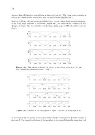
![161
frequency, because
i0−3n = ia−3n + ib−3n + ic−3n =
= an cos(3nωt + γn) + an cos(3nωt + γn + 120◦
) + (14.4)
+ an cos(3nωt + γn − 120◦
) = 3an cos(3nωt + γn)
For the other harmonics, the current in the different phases are cancelling one another in
the neutral conductor since each of them represents a symmetrical phase sequence
0 20 40 60 80 100 120 140 160 180
0
0.5
1
1.5
2
RMS(ia) RMS(i0)
RMS(i0) / RMS(ia)
alfa [degrees]
Figure 14.6. RMS(ia) (’—’), RMS(i0) (’- - -’), and the quotient RMS(i0)/RMS(ia) (’...’)
i0−(3n±1) = ia−(3n±1) + ib−(3n±1) + ic−(3n±1) =
= an cos(3nωt + γn) + an cos(3nωt + γn ± 120◦
) + (14.5)
+ an cos(3nωt + γn 120◦
) = 0
Note that if no neutral conductor existed, no harmonics having a multiple of three times the
fundamental frequency could occur in the phase conductors either. Since the harmonics of
multiples of three times the fundamental frequency has the same phase position, they will
appear as zero-sequence components which implies that they cannot pass ∆-Y-connected
transformers.
The firing angle of the thyristors will of course influence the currents in the phases as well as
in the neutral conductor. In Figure 14.6, the change in the RMS-value of the current when
the firing angle is increased is shown.
As shown in Figure 14.6, the i0-current is relatively small for firing angles up to approximately
20◦
. When the firing angle has increased to about 70◦
, the RMS-values of the current in the
neutral conductor is as large as the RMS-value of the phase current. The RMS-value of the
current in the neutral conductor reach a maximum value when the firing angle is α = 90◦
and for even higher firing angles, the current in the neutral conductor is
√
3 times the phase
current.](https://image.slidesharecdn.com/staticanalysisofpowersystems-150222152940-conversion-gate02/85/Static-analysis-of-power-systems-167-320.jpg)

![Appendix A
MATLAB-codes for Examples 7.2, 7.3, 13.2
and 13.3
%--- Example 7.2
% File name: Ex7_2.m
clear%
deg=180/pi;%
rad=1/deg;
% Choose the base values
Sb=0.5; Ub10=10; Ib10=Sb/Ub10/sqrt(3);Zb10=Ub10^2/Sb;%
Ub70=70; Ib70=Sb/Ub70/sqrt(3);
%Calculate the per-unit values of the Th´evenin equivalent of the system
UTh=70*exp(j*0*rad); Isc=0.3*exp(j*-90*rad);%
UThpu =UTh/Ub70; Iscpu =Isc/Ib70; ZThpu =UThpu/Iscpu;
% Calculate the per-unit values of the transformer
Zt=j*4/100;Snt=5; Ztpu=Zt*Sb/Snt;
%Calculate the per-unit values of the line
Z21pu=5*(0.9+j*0.3)/Zb10; ysh21pu=5*(j*3*1E-6)*Zb10/2;
%Calculate the per-unit values of the industry impedance
cosphi=0.8; sinphi=sqrt(1-cosphi^2);%
Un=Ub10; PLD=0.4;absSLD=PLD/cosphi; SLD=absSLD*(cosphi+j*sinphi);%
ZLDpu=Un^2/conj(SLD)/Zb10
% The twoport of the system
AL=1+ysh21pu*Z21pu; BL=Z21pu; CL=ysh21pu*(2+ysh21pu*Z21pu); DL=AL;
F_L=[AL BL ; CL DL]; F_Th_tr=[1 ZThpu+Ztpu ; 0 1]; F_tot=F_Th_tr*F_L;
%The impedance of the entire system
Ztotpu=(F_tot(1,1)*ZLDpu+F_tot(1,2))/(F_tot(2,1)*ZLDpu+F_tot(2,2));%
I4pu = UThpu/Ztotpu;
%The power fed by the transformer into the line
U2pu_I2pu=inv(F_Th_tr)*[UThpu;I4pu];%
S2=U2pu_I2pu(1,1)*conj(U2pu_I2pu(2,1))*Sb
%The voltage at the industry
U1pu_I1pu=inv(F_tot)*[UThpu;I4pu];%
163](https://image.slidesharecdn.com/staticanalysisofpowersystems-150222152940-conversion-gate02/85/Static-analysis-of-power-systems-169-320.jpg)
![164
U1=abs(U1pu_I1pu(1,1))*Ub10,
%--- Example 7.3
% File name: Ex7_3.m
clear%
deg=180/pi;%
rad=1/deg;
% Choose the base values
Sb=0.5; Ub70=70; Ib70=Sb/Ub70/sqrt(3);%
Ub10=10; Ib10=Sb/Ub10/sqrt(3);Zb10=Ub10^2/Sb;%
Ub04=04; Ib04=Sb/Ub04/sqrt(3);Zb04=Ub04^2/Sb;
%Calculate the per-unit values of the infinite bus
U1=70/Ub70;
%Calculate the per-unit values of the transformer T1 and T2
Zt1=j*7/100;Snt1=0.8; Zt1pu=Zt1*Sb/Snt1;%
Zt2=j*8/100;Snt2=0.3; Zt2pu=Zt2*Sb/Snt2;
%Calculate the per-unit values of Line1and Line2
Z23pu=2*[0.17+j*0.3]/Zb10; ysh23pu=2*(3.2*1E-6)*Zb10/2;%
Z24pu=1*[0.17+j*0.3]/Zb10; ysh24pu=1*(3.2*1E-6)*Zb10/2;
%Calculate the per-unit values of the impedance LD1 and LD2
cosphiLD1=0.8; sinphiLD1=sqrt(1-cosphiLD1^2);%
UnLD1=Ub10; PLD1=0.5;absSLD1=PLD1/cosphiLD1; SLD1=absSLD1*(cosphiLD1+j*sinphiLD1);%
ZLD1pu=UnLD1^2/conj(SLD1)/Zb10
cosphiLD2=0.95; sinphiLD2=sqrt(1-cosphiLD2^2);%
UnLD2=Ub04;PLD2=0.2;absSLD2=PLD2/cosphiLD2; SLD2=absSLD2*(cosphiLD2+j*sinphiLD2);%
ZLD2pu=UnLD2^2/conj(SLD2)/Zb04
%Y-BUS
Y22=1/Zt1pu+1/Z23pu+ysh23pu+1/Z24pu+ysh24pu;%
Y33=1/Z23pu+ysh23pu+1/ZLD1pu;%
Y44=1/Z24pu+ysh24pu+1/Zt2pu;
Ybus=[ 1/Zt1pu -1/Zt1pu 0 0 0;
-1/Zt1pu Y22 -1/Z23pu -1/Z24pu 0;
0 -1/Z23pu Y33 0 0;
0 -1/Z24pu 0 Y44 -1/Zt2pu;
0 0 0 -1/Zt2pu 1/Zt2pu+1/ZLD2pu];
Zbus=inv(Ybus);
%Calculate the efficiency
I1=U1/Zbus(1,1);%](https://image.slidesharecdn.com/staticanalysisofpowersystems-150222152940-conversion-gate02/85/Static-analysis-of-power-systems-170-320.jpg)
![166
% 2)
UThbus1=UTh/A_1; ZThbus1_1=B_1/A_1; ZThbus1_2=ZThbus1_1;
F_tot_0=[ 1 Zt_0 ; 0 1]*[AL_0 BL_0 ; CL_0 DL_0];%
ZThbus1_0=F_tot_0(1,2)/F_tot_0(1,1);
% 3)
alfa=exp(j*120*rad); TT=[1 1 1 ; alfa^2 alfa 1 ; alfa alfa^2 1];%
ZLDs=inv(TT)*[2*ZLDpu 0 0 ; 0 ZLDpu 0 ; 0 0 ZLDpu]*TT;%
UTH=[UThbus1 ; 0 ; 0];%
Zs=[ZThbus1_1 0 0 ; 0 ZThbus1_2 0 ; 0 0 ZThbus1_0];%
Is=inv(Zs+ZLDs)*UTH;
% 4-5)
Ubus1s=ZLDs*Is;%
Ubus2_Ibus2_1=[AL_1 BL_1 ; CL_1 DL_1]*[Ubus1s(1) ; Is(1)];%
Ubus2_Ibus2_2=[AL_2 BL_2 ; CL_2 DL_2]*[Ubus1s(2) ; Is(2)];%
Ubus2_Ibus2_0=[AL_0 BL_0 ; CL_0 DL_0]*[Ubus1s(3) ; Is(3)];%
Sbus2_1=Ubus2_Ibus2_1(1,1)*conj(Ubus2_Ibus2_1(2,1))*Sb;%
Sbus2_2=Ubus2_Ibus2_2(1,1)*conj(Ubus2_Ibus2_2(2,1))*Sb;%
Sbus2_0=Ubus2_Ibus2_0(1,1)*conj(Ubus2_Ibus2_0(2,1))*Sb;
% 6)
Ubus1_Ph=[abs(TT*Ubus1s*Ub10/sqrt(3)) angle(TT*Ubus1s*Ub10/sqrt(3))*deg]%
Stot=Sbus2_1+Sbus2_2+Sbus2_0
%--- Example 13.3
% File name: Ex13_3
clear
Ex7_3, %Run Example 7.3
% 1)
% Positive- and negative-sequence components in per-unit values (from the
% solution to Example 7.3)
UTh=U1;
Zt1_1=Zt1pu ; Zt1_2=Zt1_1;%
Zt2_1=Zt2pu ; Zt2_2=Zt2_1;%
Z23_1=Z23pu ; Z23_2=Z23_1;%
ysh23_1=ysh23pu ; ysh23_2=ysh23_1;%
Z24_1=Z24pu ; Z24_2=Z24_1;%
ysh24_1=ysh24pu ; ysh24_2=ysh24_1;%
ZLD1_1=ZLD1pu ; ZLD1_2=ZLD1_1;%
%Zero-sequence components in per-unit values
Zt1_0=Zt1_1 ; Zt2_0=Zt2_1;%
Z23_0=3*Z23_1 ; ysh23_0=0.5*ysh23_1;%](https://image.slidesharecdn.com/staticanalysisofpowersystems-150222152940-conversion-gate02/85/Static-analysis-of-power-systems-172-320.jpg)
![167
Z24_0=3*Z24_1 ; ysh24_0=0.5*ysh24_1;%
% 2)
Y1=Ybus; Y1(5,5)=1/Zt2_1; Z1=inv(Y1);%
Ibus1_1=UTh/Z1(1,1); UThbus5=Z1(5,1)*Ibus1_1;%
YD1=Y1(2:5,2:5); ZD1=inv(YD1); ZD2=ZD1;
% 3)
ZThbus5_1=ZD1(5-1,5-1); ZThbus5_2=ZThbus5_1;
Y22_0=1/Zt1_0+1/Z23_0+ysh23_0+1/Z24_0+ysh24_0;%
Y33_0=1/Z23_0+ysh23_0;%
Y44_0=1/Z24_0+ysh24_0+1/Zt2_0;
YD0=[ Y22_0 -1/Z23_0 -1/Z24_0 0;
-1/Z23_0 Y33_0 0 0;
-1/Z24_0 0 Y44_0 -1/Zt2_0;
0 0 -1/Zt2_0 1/Zt2_0];
ZD0=inv(YD0); ZThbus5_0=ZD0(5-1,5-1);
UPre_5=[UThbus5 ; 0 ; 0];%
ZD_5=[ZThbus5_1 0 0 ; 0 ZThbus5_2 0 ; 0 0 ZThbus5_0];%
alfa=exp(j*120*rad);%
TT=[1 1 1 ; alfa^2 alfa 1 ; alfa alfa^2 1];%
ZLDbus5s=inv(TT)*[2*ZLD2pu 0 0 ; 0 ZLD2pu 0 ; 0 0 ZLD2pu]*TT;%
ID_5=-inv(ZD_5+ZLDbus5s)*UPre_5;
% 4)
Up2_1=Z1(2,1)*Ibus1_1+ ZD1(2-1,5-1)*ID_5(1);%
Up2_2= 0 + ZD2(2-1,5-1)*ID_5(2);%
Up2_0= 0 + ZD0(2-1,5-1)*ID_5(3);%
Up3_1=Z1(3,1)*Ibus1_1+ ZD1(3-1,5-1)*ID_5(1);%
Up3_2= 0 + ZD2(3-1,5-1)*ID_5(2);%
Up3_0= 0 + ZD0(3-1,5-1)*ID_5(3);%
Up4_1=Z1(4,1)*Ibus1_1+ ZD1(4-1,5-1)*ID_5(1);%
Up4_2= 0 + ZD2(4-1,5-1)*ID_5(2);%
Up4_0= 0 + ZD0(4-1,5-1)*ID_5(3);%
Up5_1=Z1(5,1)*Ibus1_1+ ZD1(5-1,5-1)*ID_5(1);%
Up5_2= 0 + ZD2(5-1,5-1)*ID_5(2);%
Up5_0= 0 + ZD0(5-1,5-1)*ID_5(3);
IZ23_1=(Up2_1-Up3_1)/Z23_1; IZ23_2=(Up2_2-Up3_2)/Z23_2; IZ23_0=(Up2_0-Up3_0)/Z23_0;%
IZ24_1=(Up2_1-Up4_1)/Z24_1; IZ24_2=(Up2_2-Up4_2)/Z24_2; IZ24_0=(Up2_0-Up4_0)/Z24_0;
SZ23_1=Up2_1*conj(IZ23_1); SZ23_2=Up2_2*conj(IZ23_2); SZ23_0=Up2_0*conj(IZ23_0);%
SZ23_in=SZ23_1+SZ23_2+SZ23_0;%
SZ24_in=Up2_1*conj(IZ24_1)+Up2_2*conj(IZ24_2)+Up2_0*conj(IZ24_0);](https://image.slidesharecdn.com/staticanalysisofpowersystems-150222152940-conversion-gate02/85/Static-analysis-of-power-systems-173-320.jpg)


![Appendix C
MATLAB-codes for Example 8.12
% Start of file
clear,%
clear global
Sb=100; Ub=220; deg=180/pi;
%Step 1
% 1a)
U1=1;theta1=0;PLD1=0.2;QLD1=0.02;%
U2=1;PG2=1;PLD2=2;QLD2=0.2;
%1b)
Z12=0.02+j*0.2;%
Y=[1/Z12 -1/Z12 ; -1/Z12 1/Z12];%
G=real(Y); B=imag(Y);%
PGD2=PG2-PLD2;
%1c)
theta2=0;
iter=0;%
while iter < 3,
iter=iter+1;
%Step 2
%2a)
P2=U1*U2*(G(2,1)*cos(theta2-theta1)+B(2,1)*sin(theta2-theta1))+U2^2*G(2,2);
%2b
deltaP=PGD2-P2;
%Step 3
Q2=U2*U1*(G(2,1)*sin(theta2-theta1)-B(2,1)*cos(theta2-theta1))-U2^2*B(2,2);
H=-Q2-U2^2*B(2,2);
JAC=[H];
%Step 4
DX=inv(JAC)*[deltaP];
delta_theta2=DX;
%Step 5
theta2=theta2+delta_theta2;
end,
%Step final
P1=U1*U2*(G(1,2)*cos(theta1-theta2)+B(1,2)*sin(theta1-theta2))+U1^2*G(1,1);%
Q1=U1*U2*(G(1,2)*sin(theta1-theta2)-B(1,2)*cos(theta1-theta2))-U1^2*B(1,1);
Q2=U2*U1*(G(2,1)*sin(theta2-theta1)-B(2,1)*cos(theta2-theta1))-U2^2*B(2,2);
171](https://image.slidesharecdn.com/staticanalysisofpowersystems-150222152940-conversion-gate02/85/Static-analysis-of-power-systems-177-320.jpg)
![172
PG1=(P1+PLD1)*Sb; QG1=(Q1+QLD1)*Sb; QG2=(Q2+QLD2)*Sb;
g=-G;b=-B;bsh_12=0;
P_12=(U1^2*g(1,2)-U1*U2*(g(1,2)*cos(theta1-theta2)+b(1,2)*sin(theta1-theta2)))*Sb;
P_21=(U2^2*g(2,1)-U2*U1*(g(2,1)*cos(theta2-theta1)+b(2,1)*sin(theta2-theta1)))*Sb;
Q_12=((-bsh_12-b(1,2))*U1^2-...
U1*U2*(g(1,2)*sin(theta1-theta2)-b(1,2)*cos(theta1-theta2)))*Sb;
Q_21=((-bsh_12-b(2,1))*U2^2-...
U2*U1*(g(2,1)*sin(theta2-theta1)-b(2,1)*cos(theta2-theta1)))*Sb;
PLoss=P_12+P_21; %or PLoss=(PG1+PG2)-(PLD1+PLD2)*Sb;
ANG=[theta1 theta2]’*deg;
VOLT=[U1 U2]*Ub;
% End of file](https://image.slidesharecdn.com/staticanalysisofpowersystems-150222152940-conversion-gate02/85/Static-analysis-of-power-systems-178-320.jpg)
![Appendix D
MATLAB-codes for Example 8.13
% Start of file
clear,%
clear global
tole=1e-6;
Sb=100; Ub=220; deg=180/pi;
%Step 1
% 1a)
U1=1;theta1=0;PLD1=0.2;QLD1=0.02;
PG2=1;QG2=0.405255;PLD2=2;QLD2=0.2;
%1b)
Z12=0.02+j*0.2;
Y=[1/Z12 -1/Z12 ; -1/Z12 1/Z12];
G=real(Y); B=imag(Y);
PGD2=PG2-PLD2;
QGD2=QG2-QLD2;
%1c)
theta2=0;
U2=1;
P2=U1*U2*(G(2,1)*cos(theta2-theta1)+B(2,1)*sin(theta2-theta1))+U2^2*G(2,2);
Q2=U2*U1*(G(2,1)*sin(theta2-theta1)-B(2,1)*cos(theta2-theta1))-U2^2*B(2,2);
deltaP=PGD2-P2;
deltaQ=QGD2-Q2;
while all(abs([deltaP;deltaQ])> tole),
%Step 2
%2a)
P2=U1*U2*(G(2,1)*cos(theta2-theta1)+B(2,1)*sin(theta2-theta1))+U2^2*G(2,2);
Q2=U2*U1*(G(2,1)*sin(theta2-theta1)-B(2,1)*cos(theta2-theta1))-U2^2*B(2,2);
%2b
deltaP=PGD2-P2,
deltaQ=QGD2-Q2,
%Step 3
H=-Q2-B(2,2)*U2^2;
N=P2+G(2,2)*U2^2;
J=P2-G(2,2)*U2^2;
L=Q2-B(2,2)*U2^2;
JAC=[H N ; J L];
%Step 4
DX=inv(JAC)*[deltaP;deltaQ];
173](https://image.slidesharecdn.com/staticanalysisofpowersystems-150222152940-conversion-gate02/85/Static-analysis-of-power-systems-179-320.jpg)
![174
delta_theta2=DX(1);
delta_U2=DX(2);
%Step 5
theta2=theta2+delta_theta2;
U2=U2*(1+delta_U2/U2);
end, %while
%Step final
P1=U1*U2*(G(1,2)*cos(theta1-theta2)+B(1,2)*sin(theta1-theta2))+U1^2*G(1,1);%
Q1=U1*U2*(G(1,2)*sin(theta1-theta2)-B(1,2)*cos(theta1-theta2))-U1^2*B(1,1);
Q2=U2*U1*(G(2,1)*sin(theta2-theta1)-B(2,1)*cos(theta2-theta1))-U2^2*B(2,2);
PG1=(P1+PLD1)*Sb; QG1=(Q1+QLD1)*Sb; QG2=(Q2+QLD2)*Sb;
g=-G;b=-B;bsh_12=0;
P_12=(U1^2*g(1,2)-U1*U2*(g(1,2)*cos(theta1-theta2)+b(1,2)*sin(theta1-theta2)))*Sb;
P_21=(U2^2*g(2,1)-U2*U1*(g(2,1)*cos(theta2-theta1)+b(2,1)*sin(theta2-theta1)))*Sb;
Q_12=((-bsh_12-b(1,2))*U1^2-...
U1*U2*(g(1,2)*sin(theta1-theta2)-b(1,2)*cos(theta1-theta2)))*Sb;
Q_21=((-bsh_12-b(2,1))*U2^2-...
U2*U1*(g(2,1)*sin(theta2-theta1)-b(2,1)*cos(theta2-theta1)))*Sb;
PLoss=P_12+P_21; %or PLoss=(PG1+PG2)-(PLD1+PLD2)*Sb;
ANG=[theta1 theta2]’*deg;
VOLT=[U1 U2]*Ub;
% End of file](https://image.slidesharecdn.com/staticanalysisofpowersystems-150222152940-conversion-gate02/85/Static-analysis-of-power-systems-180-320.jpg)
![Appendix E
MATLAB-codes for Example 8.14
% To run Load Flow (LF), two MATLAB-files are used, namely
% (run_LF.m) and (solve_lf.m)
% Start of file (run_LF.m)
clear%
clear global
%%%%%%%%%%%%%%%%%%%%%%%%%%
tole=1e-9; deg=180/pi; rad=1/deg ;
%%%%%%%%%%%%%%
% Base values
%%%%%%%%%%%%%%
Sb=100; Ub=220; Zb=Ub^2/Sb;
%%%%%%%%%%%%
% Bus data
%%%%%%%%%%%%
% Number of buses
nbus=4;
%Bus 1, slack bus
U1=220/Ub; theta1=0*rad; PLD1=10/Sb; QLD1=2/Sb;
%Bus 2, PQ-bus
PG2=0/Sb; QG2=0/Sb; PLD2=90/Sb; QLD2=10/Sb;
%Bus 3, PQ-bus
PG3=0/Sb; QG3=0/Sb; PLD3=80/Sb; QLD3=10/Sb;
%Bus 4, PQ-bus
PG4=0/Sb; QG4=0/Sb; PLD4=50/Sb; QLD4=10/Sb;
%%%%%%%%%%%%
% Line data
%%%%%%%%%%%%
Z12=(5+j*65)/Zb;bsh12=0.0002*Zb;%
Z13=(4+j*60)/Zb;bsh13=0.0002*Zb;%
Z23=(5+j*68)/Zb;bsh23=0.0002*Zb;%
Z34=(3+j*30)/Zb;bsh34=0;
%%%%%%%%%%%%%%
% YBUS matrix
%%%%%%%%%%%%%%
y11=1/Z12+1/Z13+j*bsh12+j*bsh13; y12=-1/Z12; y13=-1/Z13; y14=0;%
y21=-1/Z12; y22=1/Z12+1/Z23+j*bsh12+j*bsh23; y23=-1/Z23; y24=0;%
y31=-1/Z13; y32=-1/Z23; y33=1/Z13+1/Z23+1/Z34+j*bsh13+j*bsh23; y34=-1/Z34;%
y41=0; y42=0; y43=-1/Z34; y44=1/Z34;%
YBUS=[y11 y12 y13 y14; y21 y22 y23 y24; y31 y32 y33 y34; y41 y42 y43 y44];%
G=real(YBUS); B=imag(YBUS);
175](https://image.slidesharecdn.com/staticanalysisofpowersystems-150222152940-conversion-gate02/85/Static-analysis-of-power-systems-181-320.jpg)
![176
%%%%%%%%%%%%%%%%%%%%%%%%%%%%%%%%%%
% Define PGD for PU- and PQ-buses
%%%%%%%%%%%%%%%%%%%%%%%%%%%%%%%%%%
PGD2=PG2-PLD2; % for bus 2 (PQ-bus)
PGD3=PG3-PLD3; % for bus 3 (PQ-bus)
PGD4=PG4-PLD4; % for bus 4 (PQ-bus)
PGD=[PGD2 ; PGD3 ; PGD4];
%%%%%%%%%%%%%%%%%%%%%%%%%%
% Define QGD for PQ-buses
%%%%%%%%%%%%%%%%%%%%%%%%%%
QGD2=QG2-QLD2; % for bus 2 (PQ-bus)
QGD3=QG3-QLD3; % for bus 3 (PQ-bus)
QGD4=QG4-QLD4; % for bus 4 (PQ-bus)
QGD=[QGD2 ; QGD3 ; QGD4];
%%%%%%%%%%%%%%%%%%%%%%%%%%%%%%%%%%%%%%%%%%%%%%%%%
% Use fsolve function in MATLAB to run load flow
%%%%%%%%%%%%%%%%%%%%%%%%%%%%%%%%%%%%%%%%%%%%%%%%%
% Unknown variables [theta2 theta3 theta4 U2 U3 U4]’;
% Define the initial values of the unknown variables
X0=[0 0 0 1 1 1]’; % Flat initial values
s_z=size(X0);
nx=s_z(1,1); % number of unknown variables
% The function below is used for fsolve (type "help fsolve" in MATLAB)
options_solve=optimset(’Display’,’off’,’TolX’,tole,’TolFun’,tole);
% Parameters used for fsolve
PAR=[nx ; nbus ; U1 ; theta1];%
[X_X]=fsolve(’solve_lf’,X0,options_solve,G,B,PGD,QGD,PAR);
% Solved variables X_X=[theta2 theta3 theta4 U2 U3 U4]’;
ANG=[theta1 X_X(1) X_X(2) X_X(3)]’;%
VOLT=[U1 X_X(4) X_X(5) X_X(6)]’,
ANG_deg=ANG*deg;%
VOLT_kV=VOLT*Ub;
%%%%%%%%%%%%%%%%%
%Jacobian matrix
%%%%%%%%%%%%%%%%%
for m=1:nbus
for n=1:nbus
PP(m,n)=VOLT(m)*VOLT(n)*(G(m,n)*cos(ANG(m)-ANG(n))+B(m,n)*sin(ANG(m)-ANG(n)));
QQ(m,n)=VOLT(m)*VOLT(n)*(G(m,n)*sin(ANG(m)-ANG(n))-B(m,n)*cos(ANG(m)-ANG(n)));
end, %for n
end, % for m
P=sum(PP’); Q=sum(QQ’);](https://image.slidesharecdn.com/staticanalysisofpowersystems-150222152940-conversion-gate02/85/Static-analysis-of-power-systems-182-320.jpg)
![177
for m=1:nbus
for n=1:nbus
if m==n,
H(m,m)=-Q(m)-B(m,m)*VOLT(m)*VOLT(m);
N(m,m)= P(m)+G(m,m)*VOLT(m)*VOLT(m);
J(m,m)= P(m)-G(m,m)*VOLT(m)*VOLT(m);
L(m,m)= Q(m)-B(m,m)*VOLT(m)*VOLT(m);
else
H(m,n)= VOLT(m)*VOLT(n)*(G(m,n)*sin(ANG(m)-ANG(n))-B(m,n)*cos(ANG(m)-ANG(n)));
N(m,n)= VOLT(m)*VOLT(n)*(G(m,n)*cos(ANG(m)-ANG(n))+B(m,n)*sin(ANG(m)-ANG(n)));
J(m,n)=-VOLT(m)*VOLT(n)*(G(m,n)*cos(ANG(m)-ANG(n))+B(m,n)*sin(ANG(m)-ANG(n)));
L(m,n)= VOLT(m)*VOLT(n)*(G(m,n)*sin(ANG(m)-ANG(n))-B(m,n)*cos(ANG(m)-ANG(n)));
end, %if
end, %for n
end, % for m
slack_bus=1; %bus 1
PU_bus=[ ]; % No buses
% Remove row and column corresponding to slack bus
H(slack_bus,:)=[ ]; H(:,slack_bus)=[ ];
% Remove row corresponding to slack bus
N(slack_bus,:)=[ ];
% Remove columns corresponding to slack bus and PU-buses
N(:,sort([slack_bus PU_bus]))=[ ];
% Remove rows corresponding to slack bus and PU-buses
J(sort([slack_bus PU_bus]),:)=[ ];
% Remove column corresponding to slack bus
J(:,slack_bus)=[ ];
%Remove rows and columns corresponding to slack bus and PU-buses
L(sort([slack_bus PU_bus]),:)=[ ]; L(:,sort([slack_bus PU_bus]))=[ ];
JAC=[H N ; J L],
%%%%%%%%%%%%%%%%%%%%%%%%%%%%%%%%%%%%%%%%%%%%%%%%%%%%%%%%%%%%%%%%%%
% The generated active and reactive power at slack bus and PU-buses
%%%%%%%%%%%%%%%%%%%%%%%%%%%%%%%%%%%%%%%%%%%%%%%%%%%%%%%%%%%%%%%%%
g=-G;b=-B;
% At slack bus, bus 1
P12=g(1,2)*VOLT(1)^2-...
VOLT(1)*VOLT(2)*(g(1,2)*cos(ANG(1)-ANG(2))+b(1,2)*sin(ANG(1)-ANG(2)));
P13=g(1,3)*VOLT(1)^2-...
VOLT(1)*VOLT(3)*(g(1,3)*cos(ANG(1)-ANG(3))+b(1,3)*sin(ANG(1)-ANG(3)));
Q12=(-bsh12-b(1,2))*VOLT(1)^2-...
VOLT(1)*VOLT(2)*(g(1,2)*sin(ANG(1)-ANG(2))-b(1,2)*cos(ANG(1)-ANG(2)));
Q13=(-bsh13-b(1,3))*VOLT(1)^2-...](https://image.slidesharecdn.com/staticanalysisofpowersystems-150222152940-conversion-gate02/85/Static-analysis-of-power-systems-183-320.jpg)
![178
VOLT(1)*VOLT(3)*(g(1,3)*sin(ANG(1)-ANG(3))-b(1,3)*cos(ANG(1)-ANG(3)));%
PG1=P12+P13+PLD1;%
QG1=Q12+Q13+QLD1;%
PG1_MW=PG1*Sb;%
QG1_MVAr=QG1*Sb;
%%%%%%%%%%%%%%%%%%%%%%%%%%%%%%%%%
% or
%PG_slackbus_MW=(P(slack_bus)+PLD1)*Sb,
%QG_slackbus_MW=(Q(slack_bus)+QLD1)*Sb,
%%%%%%%%%%%%%%%%%%%%%%%%%%%%%%%%%
%%%%%%%%%
% Losses
%%%%%%%%%
PLoss_tot=(PG1+PG2+PG3+PG4)-(PLD1+PLD2+PLD3+PLD4);%
PLoss_tot_MW=PLoss_tot*Sb;
P34=g(3,4)*VOLT(3)^2-...
VOLT(3)*VOLT(4)*(g(3,4)*cos(ANG(3)-ANG(4))+b(3,4)*sin(ANG(3)-ANG(4)));
P43=g(4,3)*VOLT(4)^2-...
VOLT(4)*VOLT(3)*(g(4,3)*cos(ANG(4)-ANG(3))+b(4,3)*sin(ANG(4)-ANG(3)));%
PLoss_Sys1=(P34+P43);%
PLoss_Sys1_MW=(P34+P43)*Sb;
PLoss_Sys2_MW=PLoss_tot_MW-PLoss_Sys1_MW;
% End of file (run_LF.m)
%%%%%%%%%%%%%%
% Second file
%%%%%%%%%%%%%%
% Start of file (solve_lf.m)
% This function solves g(x)=0 for x.
function [g_x]=solve_lf(X,G,B,PGD,QGD,PAR);
nx=PAR(1); nbus=PAR(2); U1=PAR(3); theta1=PAR(4);
PGD2=PGD(1); PGD3=PGD(2); PGD4=PGD(3); QGD2=QGD(1); QGD3=QGD(2); QGD4=QGD(3);
theta2=X(1); theta3=X(2); theta4=X(3); U2=X(4); U3=X(5); U4=X(6);
ANG=[theta1 theta2 theta3 theta4]’ ; VOLT=[U1 U2 U3 U4]’;](https://image.slidesharecdn.com/staticanalysisofpowersystems-150222152940-conversion-gate02/85/Static-analysis-of-power-systems-184-320.jpg)

![Appendix F
MATLAB-codes for Example 8.15
Note that only the changes of the MATLAB-codes compared to the MATLAB-codes for
Example 8.14 are given in this appendix.
% Changes in file run_LF.m
%%%%%%%%%%%%
% Bus data
%%%%%%%%%%%%
% Number of buses
nbus=4;
%Bus 3, PU-bus
PG3=0/Sb; U3=220/Ub; PLD3=80/Sb; QLD3=10/Sb;
%%%%%%%%%%%%
% Line data
%%%%%%%%%%%%
%%%%%%%%%%%%%%
% YBUS matrix
%%%%%%%%%%%%%%
%%%%%%%%%%%%%%%%%%%%%%%%%%%%%%%%%%
% Define PGD for PU- and PQ-buses
%%%%%%%%%%%%%%%%%%%%%%%%%%%%%%%%%%
%%%%%%%%%%%%%%%%%%%%%%%%%%
% Define QGD for PQ-buses
%%%%%%%%%%%%%%%%%%%%%%%%%%
QGD2=QG2-QLD2; % for bus 2 (PQ-bus)
QGD4=QG4-QLD4; % for bus 4 (PQ-bus)
QGD=[QGD2 ; QGD4];
%%%%%%%%%%%%%%%%%%%%%%%%%%%%%%%%%%%%%%%%%%%%%%%%%
% Use fsolve function in MATLAB to run load flow
%%%%%%%%%%%%%%%%%%%%%%%%%%%%%%%%%%%%%%%%%%%%%%%%%
% Unknown variables [theta2 theta3 theta4 U2 U4]’;
% Define the initial values of the unknown variables
X0=[0 0 0 1 1]’; % Flat initial values
% Parameters used for fsolve
PAR=[nx ; nbus ; U1 ; U3 ; theta1];%
181](https://image.slidesharecdn.com/staticanalysisofpowersystems-150222152940-conversion-gate02/85/Static-analysis-of-power-systems-187-320.jpg)
![182
% Solved variables X_X=[theta1 theta2 theta4 U2 U4]’;
ANG=[theta1 X_X(1) X_X(2) X_X(3)]’;%
VOLT=[U1 X_X(4) U3 X_X(5)]’;
%%%%%%%%%%%%%%%%%
%Jacobian matrix
%%%%%%%%%%%%%%%%%
slack_bus=1; %bus 1
PU_bus=[3]; %bus 3
%%%%%%%%%%%%%%%%%%%%%%%%%%%%%%%%%%%%%%%%%%%%%%%%%%%%%%%%%%%%%%%%%%
% The generated active and reactive power at slack bus and PU-buses
%%%%%%%%%%%%%%%%%%%%%%%%%%%%%%%%%%%%%%%%%%%%%%%%%%%%%%%%%%%%%%%%%
g=-G;b=-B;
% At slack bus, bus 1
% At PU-buses, bus 3
Q31=(-bsh13-b(3,1))*VOLT(3)^2-...
VOLT(3)*VOLT(1)*(g(3,1)*sin(ANG(3)-ANG(1))-b(3,1)*cos(ANG(3)-ANG(1)));
Q32=(-bsh23-b(3,2))*VOLT(3)^2-...
VOLT(3)*VOLT(2)*(g(3,2)*sin(ANG(3)-ANG(2))-b(3,2)*cos(ANG(3)-ANG(2)));
Q34=(-bsh34-b(3,4))*VOLT(3)^2-...
VOLT(3)*VOLT(4)*(g(3,4)*sin(ANG(3)-ANG(4))-b(3,4)*cos(ANG(3)-ANG(4)));%
QG3=Q31+Q32+Q34+QLD3;%
QG3_MVAr=QG3*Sb;
%%%%%%%%%%%%%%%%%%%%%%%%%%%%%%%%
% or
%QLD_pubus=[QLD3];
%QG_pubus_MVAr=(Q(PU_bus’)+QLD_pubus’)*Sb,
%%%%%%%%%%%%%%%%%%%%%%%%%%%%%%%%
%%%%%%%%%
% Losses
%%%%%%%%%
% End of file (run_LF.m)](https://image.slidesharecdn.com/staticanalysisofpowersystems-150222152940-conversion-gate02/85/Static-analysis-of-power-systems-188-320.jpg)
![183
%%%%%%%%%%%%%%
% Second file
%%%%%%%%%%%%%%
% Start of file (solve_lf.m)
function [g_x]=solve_lf(X,G,B,PGD,QGD,PAR);
nx=PAR(1); nbus=PAR(2); U1=PAR(3); U3=PAR(4); theta1=PAR(5);
PGD2=PGD(1); PGD3=PGD(2); PGD4=PGD(3); QGD2=QGD(1); QGD4=QGD(2);
theta2=X(1); theta3=X(2); theta4=X(3); U2=X(4); U4=X(5);
ANG=[theta1 theta2 theta3 theta4]’; VOLT=[U1 U2 U3 U4]’;
% We have nx unknown variables, therefore the
% size of g(x) is nx by 1.
g_x=zeros(nx,1);
for m=1:nbus
for n=1:nbus
PP(m,n)=VOLT(m)*VOLT(n)*(G(m,n)*cos(ANG(m)-ANG(n))+B(m,n)*sin(ANG(m)-ANG(n)));
QQ(m,n)=VOLT(m)*VOLT(n)*(G(m,n)*sin(ANG(m)-ANG(n))-B(m,n)*cos(ANG(m)-ANG(n)));
end, %for n
end, % for m
P=sum(PP’)’;
Q=sum(QQ’)’;
% Active power mismatch (PU- and PQ-buses)
% Bus 2
g_x(1)=P(2)-PGD2;
% Bus 3
g_x(2)=P(3)-PGD3;
% Bus 4
g_x(3)=P(4)-PGD4;
% Reactive power mismatch (PQ-buses)
% Bus 2
g_x(4)=Q(2)-QGD2;
% Bus 4
g_x(5)=Q(4)-QGD4;
% End of file (solve_lf.m)](https://image.slidesharecdn.com/staticanalysisofpowersystems-150222152940-conversion-gate02/85/Static-analysis-of-power-systems-189-320.jpg)