Downloaded 128 times

![©ZeusNumerix
Schemes
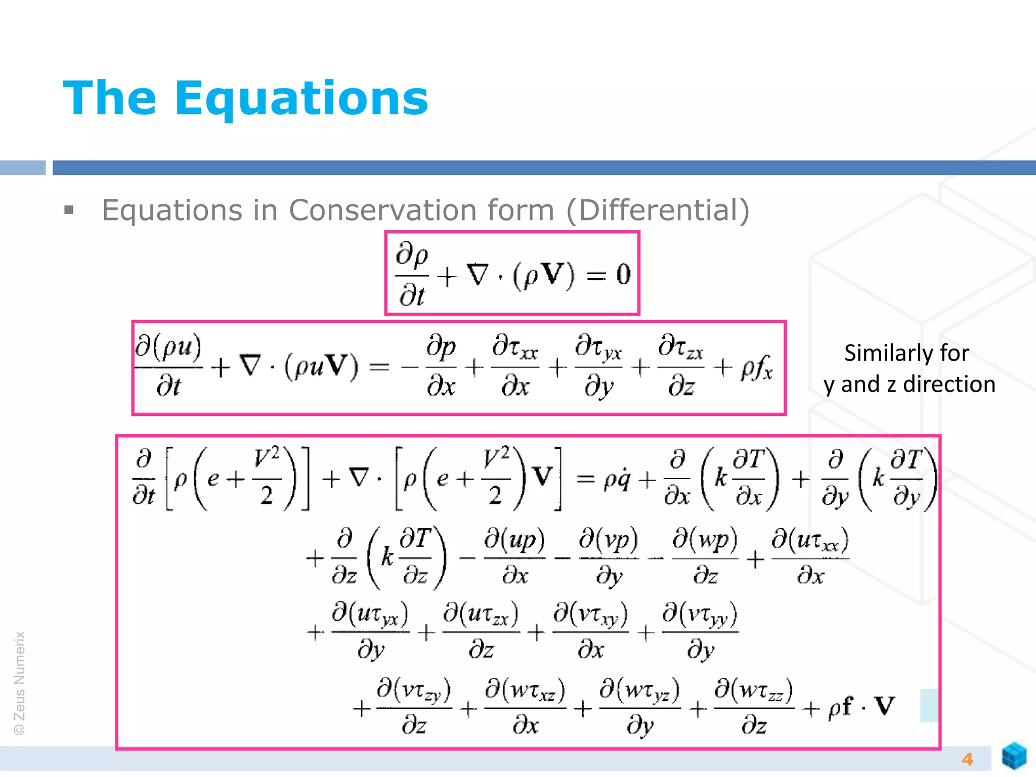
Problems in CFD can be finally simplified to
dU/dt +dF/dx = 0
Method of solving for [F] is called a scheme
Flux vector splitting schemes
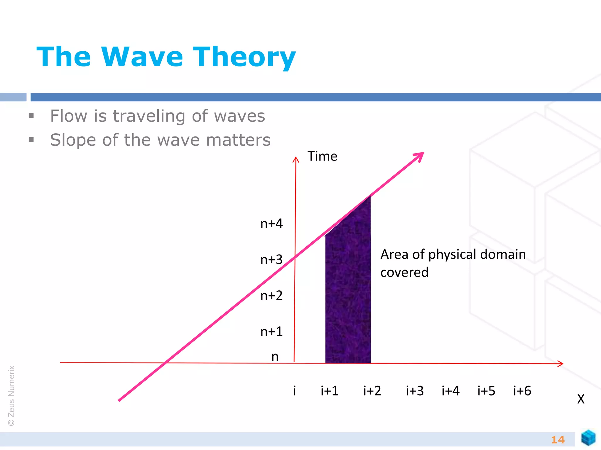
Equations contains waves that travel in forward and backward
direction
Flux vector split in such a fashion that waves are split in
forward moving and backward moving
Solved independently to get solution
Van Leer scheme – M = M++M-
Steger Warming Method – Λ = Λ++Λ-
van Leer better at sonic points as M is second derivative
16](https://image.slidesharecdn.com/compressibleflowbasics-150112004304-conversion-gate02/75/Compressible-flow-basics-16-2048.jpg)


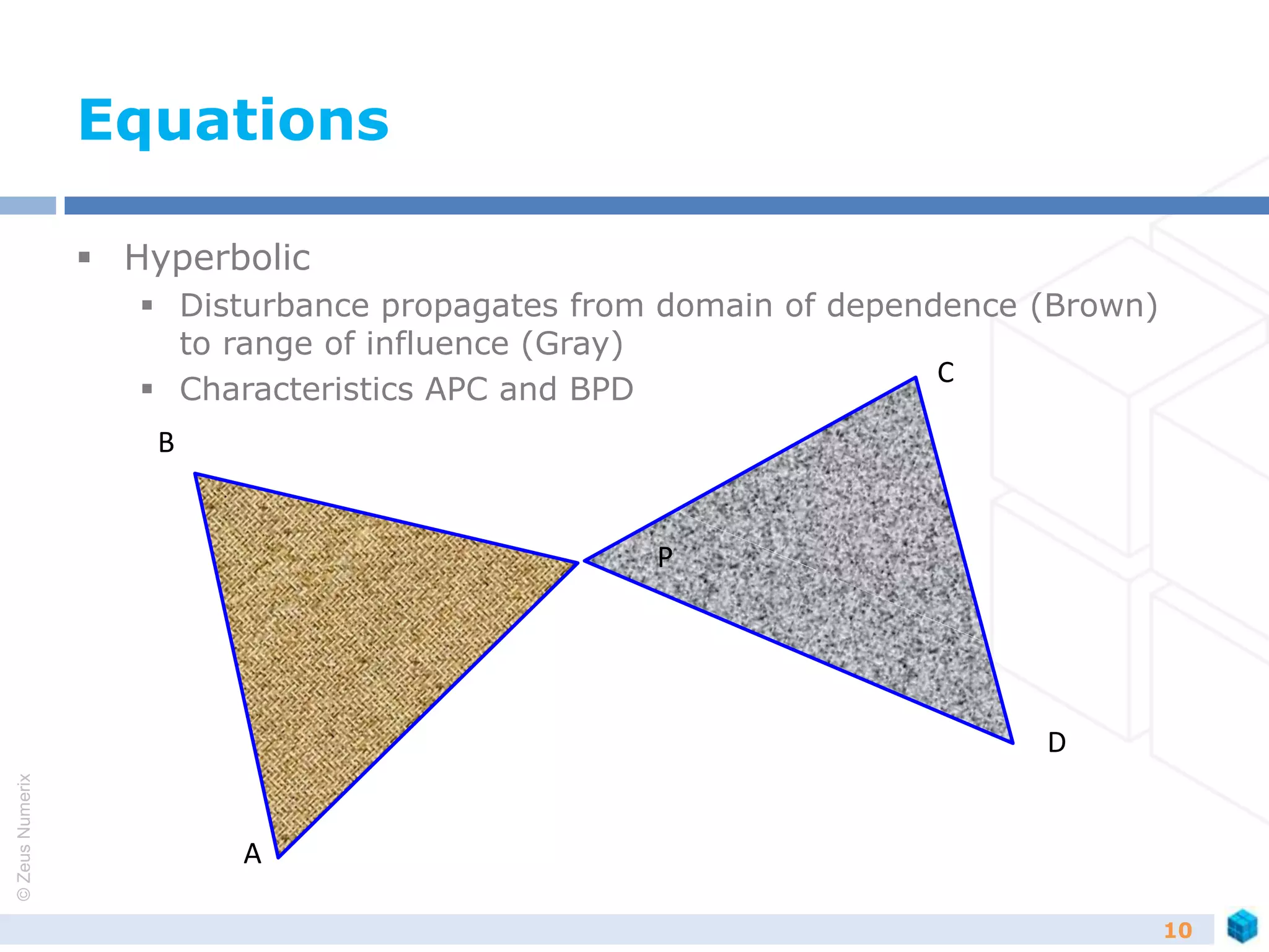
This document discusses the treatment of compressible flow in computational fluid dynamics (CFD). It covers the basics of compressible flow including conservation laws, the governing equations in conservation form, and the wave theory known as the CFL condition. It also discusses schemes for solving the equations, including flux vector splitting schemes, Roe averaged schemes, and AUSM schemes. The document emphasizes that compressible flow equations are hyperbolic and describes how characteristics and eigenvalues relate to the equation types.