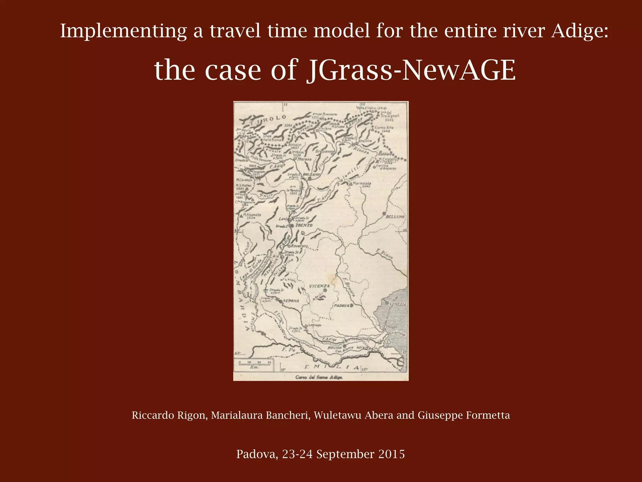
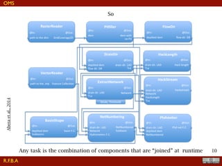
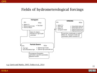
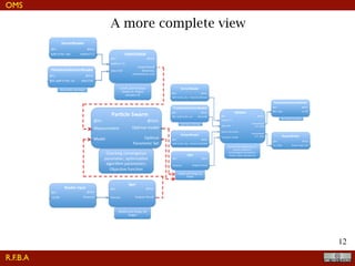
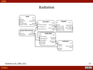
The document discusses the implementation of a travel time model for the River Adige using the JGrass-NewAGE system, highlighting the development of a database with various digital terrain data and the modelling goals including the aggregated scale of the hydrological cycle. It emphasizes the importance of component-based object-oriented software design for modelling frameworks and presents the application of the modelling components to simulate hydrological processes. The paper also illustrates the methodologies involved in parameter estimation, uncertainty analysis, and the overall structure of the modelling framework suitable for operational use.
![!34
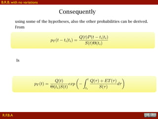
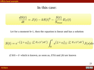
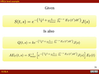
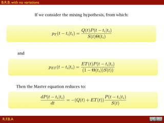
Is a linear partial differential equation which is integrable.
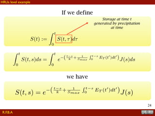
[If we make the assumptions explicated before, Q(t), ET(t) and S(t) can be
assumed to be known]
The logical initial condition is:
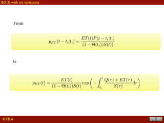
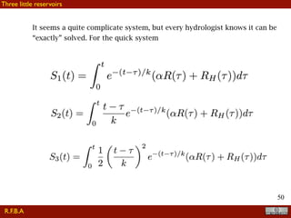
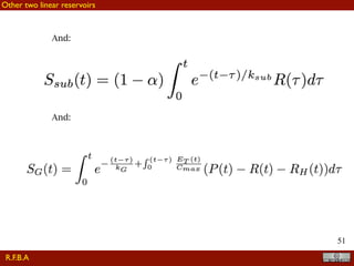
And the solution is:
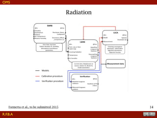
R.F.B.A
B.R.B. with no variations](https://image.slidesharecdn.com/adigemodelling-150925080125-lva1-app6891/85/Adige-modelling-34-320.jpg)