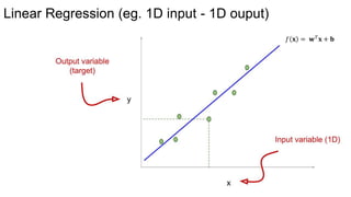
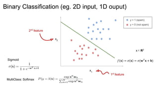
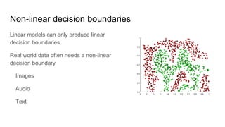
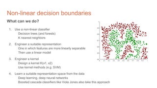
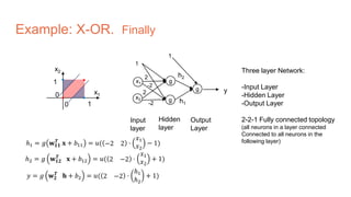
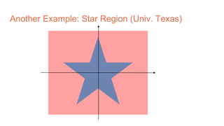
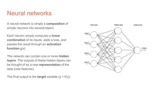
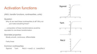
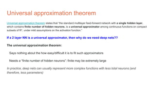
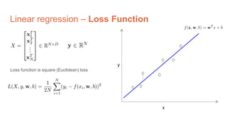
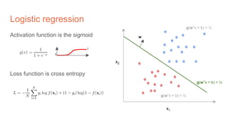
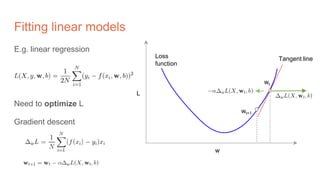
The document discusses the concepts of multilayer perceptrons and neural networks, contrasting linear and non-linear models to address real-world data that often requires non-linear decision boundaries. It explains the structure of neural networks, emphasizing the importance of activation functions and the universal approximation theorem, which asserts that multilayer networks can approximate continuous functions. Additionally, it covers training techniques such as gradient descent, validation, and accuracy metrics, highlighting the training of neural networks using specific datasets like MNIST.

1. [course site]
Day 2 Lecture 1
Multilayer Perceptron
Elisa Sayrol

2. 2
Acknowledgements
Antonio Bonafonte
Kevin McGuinness
kevin.mcguinness@dcu.ie
Research Fellow
Insight Centre for Data Analytics
Dublin City University

3. …in our last lecture

4. Linear Regression (eg. 1D input - 1D ouput)
𝑓 𝐱 = 𝐰 𝑇
𝐱 + 𝐛

5. Binary Classification (eg. 2D input, 1D ouput)
MultiClass: Softmax
𝑓 𝐱 = 𝜎 𝐱 = 𝜎(𝐰 𝑇
𝐱 + 𝐛)Sigmoid

6. Non-linear decision boundaries
Linear models can only produce linear
decision boundaries
Real world data often needs a non-linear
decision boundary
Images
Audio
Text

7. Non-linear decision boundaries
What can we do?
1. Use a non-linear classifier
Decision trees (and forests)
K nearest neighbors
2. Engineer a suitable representation
One in which features are more linearly separable
Then use a linear model
3. Engineer a kernel
Design a kernel K(x1, x2)
Use kernel methods (e.g. SVM)
4. Learn a suitable representation space from the data
Deep learning, deep neural networks
Boosted cascade classifiers like Viola Jones also take this approach

8. Example: X-OR.
AND and OR can be generated with a single perceptron
g
-3
x1
x2
2
2
y1
x1
x2 AND
0
0
1
1
g
-1
x1
x2
2
2
y2
OR
0
0
x2
1
x1
1
𝑦1 = 𝑔 𝐰 𝑻
𝐱 + 𝑏 = 𝑢( 2 2 ·
𝑥1
𝑥2
− 3) 𝑦2 = 𝑔 𝐰 𝑻
𝐱 + 𝑏 = 𝑢( 2 2 ·
𝑥1
𝑥2
− 1)
Input vector
(x1,x2)
Class
OR
(0,0) 0
(0,1) 1
(1,0) 1
(1,1) 1
Input vector
(x1,x2)
Class
AND
(0,0) 0
(0,1) 0
(1,0) 0
(1,1) 1

9. Example: X-OR
X-OR a Non-linear separable problem can not be
generated with a single perceptron
XOR
0
0
x2
1
x1
1
Input vector
(x1,x2)
Class
XOR
(0,0) 0
(0,1) 1
(1,0) 1
(1,1) 0

10. Example: X-OR. However…..
g
-1
x1
x2
-2
2
h1
x1
x2
0
0
1
1
ℎ1 = 𝑔 𝐰 𝟏𝟏
𝑻
𝐱 + 𝑏11 = 𝑢( −2 2 ·
𝑥1
𝑥2
− 1)
ℎ2 = 𝑔 𝐰 𝟏𝟐
𝑻
𝐱 + 𝑏12 = 𝑢( 2 −2 ·
𝑥1
𝑥2
+ 1)
g
-1
x1
x2
2
-2
h2
0
0
x2
1
x1
1
𝑦 = 𝑔 𝐰 𝟐
𝑻
𝐡 + 𝑏2 = 𝑢( 2 −2 ·
ℎ1
ℎ2
+ 1)
g
-1
h1
h2
2
2
y
0
h2
h1
(0,0)
(1,1)
(0,1)
(1,0)

11. Example: X-OR. Finally
x1
x2
0
0
1
1
ℎ1 = 𝑔 𝐰 𝟏𝟏
𝑻
𝐱 + 𝑏11 = 𝑢( −2 2 ·
𝑥1
𝑥2
− 1)
ℎ2 = 𝑔 𝐰 𝟏𝟐
𝑻
𝐱 + 𝑏12 = 𝑢( 2 −2 ·
𝑥1
𝑥2
+ 1)
𝑦 = 𝑔 𝐰 𝟐
𝑻
𝐡 + 𝑏2 = 𝑢( 2 −2 ·
ℎ1
ℎ2
+ 1)
g h1
g
1
x1
x2
2
-2
h2
2
-2
g
1
Input
layer
Hidden
layer
Output
Layer
y
Three layer Network:
-Input Layer
-Hidden Layer
-Output Layer
2-2-1 Fully connected topology
(all neurons in a layer connected
Connected to all neurons in the
following layer)

12. Another Example: Star Region (Univ. Texas)

13. Neural networks
A neural network is simply a composition of
simple neurons into several layers
Each neuron simply computes a linear
combination of its inputs, adds a bias, and
passes the result through an activation
function g(x)
The network can contain one or more hidden
layers. The outputs of these hidden layers can
be thought of as a new representation of the
data (new features).
The final output is the target variable (y = f(x))

14. Multilayer perceptrons
When each node in each layer is a linear
combination of all inputs from the previous
layer then the network is called a multilayer
perceptron (MLP)
Weights can be organized into matrices.
Forward pass computes
Depth
Width
𝐡(1)
=g(𝑊(1)
𝐡(1)
+𝐛(1)
)

15. Activation functions
(AKA. transfer functions, nonlinearities, units)
Question:
Why do we need these nonlinearities at all? Why not
just make everything linear?
…..composition of linear transformations would be
equivalent to one linear transformation
Desirable properties
Mostly smooth, continuous, differentiable
Fairly linear
Common nonlinearities
Sigmoid Tanh ReLU = max(0, x) LeakyReLU
Sigmoid
Tanh
ReLU

16. Universal approximation theorem
Universal approximation theorem states that “the standard multilayer feed-forward network with a single hidden layer,
which contains finite number of hidden neurons, is a universal approximator among continuous functions on compact
subsets of Rn, under mild assumptions on the activation function.”
If a 2 layer NN is a universal approximator, then why do we need deep nets??
The universal approximation theorem:
Says nothing about the how easy/difficult it is to fit such approximators
Needs a “finite number of hidden neurons”: finite may be extremely large
In practice, deep nets can usually represent more complex functions with less total neurons (and
therefore, less parameters)

17. …Learning

18. Linear regression – Loss Function
y
x
Loss function is square (Euclidean) loss

19. Logistic regression
Activation function is the sigmoid
Loss function is cross entropy
x2
x1
g(wTx + b) = ½
w
g(wTx + b) > ½
g(wTx + b) < ½
1
0

20. Fitting linear models
E.g. linear regression
Need to optimize L
Gradient descent
w
L
Tangent lineLoss
function
wt
wt+1

21. Choosing the learning rate
For first order optimization methods, we need to
choose a learning rate (aka step size)
Too large: overshoots local minimum, loss increases
Too small: makes very slow progress, can get stuck
Good learning rate: makes steady progress toward local
minimum
Usually want a higher learning rate at the start
and a lower one later on.
Common strategy in practice:
Start off with a high LR (like 0.1 - 0.001),
Run for several epochs (1 – 10)
Decrease LR by multiplying a constant factor (0.1 - 0.5)
w
L
Loss
wt
α too large
Good α
α too
small

22. Training
Estimate parameters 𝜃(W(k), b(k)) from training examples
Given a Loss Function 𝑊
∗
= 𝑎𝑟𝑔𝑚𝑖𝑛 𝜃ℒ 𝑓𝜃 𝑥 , 𝑦
In general no close form solutions:
• Iteratively adapt each parameter, numerical approximation
Basic idea: gradient descent.
• Dependencies are very complex.
Global minimum: challenging. Local minima: can be good enough.
• Initialization influences in the solutions.

23. Training
Gradient Descent: Move the parameter 𝜃𝑗in small steps in the direction opposite sign of the
derivative of the loss with respect j.
𝜃(𝑛)
= 𝜃(𝑛−1)
− 𝛼(𝑛−1)
∙ 𝛻𝜃ℒ(𝑦, 𝑓 𝑥 )
• Stochastic gradient descent (SGD): estimate the gradient with one sample, or better, with a
minibatch of examples.
• Momentum: the movement direction of parameters averages the gradient estimation with
previous ones.
Several strategies have been proposed to update the weights: Adam, RMSProp, Adamax, etc.
known as: optimizers

24. Training and monitoring progress
1. Split data into train, validation, and test sets
Keep 10-30% of data for validation
2. Fit model parameters on train set using SGD
3. After each epoch:
Test model on validation set and compute loss
Also compute whatever other metrics you are interested in
Save a snapshot of the model
4. Plot learning curves as training progresses
5. Stop when validation loss starts to increase
6. Use model with minimum validation loss
epoch
Loss
Validation loss
Training loss
Best model

25. Gradient descent examples
Linear regression
http://nbviewer.jupyter.org/github/kevinmcguinness/ml-examples/blob/master/notebooks/GD_Regression.ipynb
https://github.com/kevinmcguinness/ml-examples/blob/master/notebooks/GD_Regression.ipynb
Logistic regression
http://nbviewer.jupyter.org/github/kevinmcguinness/ml-examples/blob/master/notebooks/GD_Classification.ipynb
https://github.com/kevinmcguinness/ml-examples/blob/master/notebooks/GD_Classification.ipynb

26. MNIST Example
Handwritten digits
• 60.000 examples
• 10.000 test examples
• 10 classes (digits 0-9)
• 28x28 grayscale images(784 pixels)
• http://yann.lecun.com/exdb/mnist/
The objective is to learn a function that predicts the digit from the image

27. MNIST Example
Model
• 3 layer neural-network ( 2 hidden layers)
• Tanh units (activation function)
• 512-512-10
• Softmax on top layer
• Cross entropy Loss

28. MNIST Example
Training
• 40 epochs using min-batch SGD
• Batch Size: 128
• Leaning Rate: 0.1 (fixed)
• Takes 5 minutes to train on GPU
Accuracy Results
• 98.12% (188 errors in 10.000 test examples)
there are ways to improve accuracy…
Metrics
𝑨𝒄𝒄𝒖𝒓𝒂𝒄𝒚 =
𝑻𝑷 + 𝑻𝑵
𝑻𝑷 + 𝑻𝑵 + 𝑭𝑷 + 𝑭𝑵
there are other metrics….

29. Training MLPs
With Multiple layers we need to find the gradient of the loss function with respect to all the parameters of
the model (W(k), b(k))
These can be found using the chain rule of differentiation.
The calculations reveal that the gradient wrt. the parameters in layer k only depends on the error from the
above layer and the output from the layer below.
This means that the gradients for each layer can be computed iteratively, starting at the last layer and
propagating the error back through the network. This is known as the backpropagation algorithm.