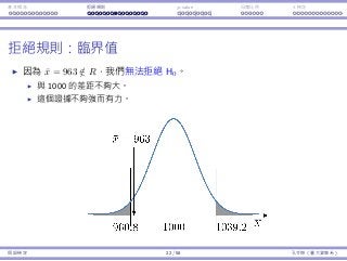
基本概念 拒絕規則 p-value⺟體比例 t 檢定
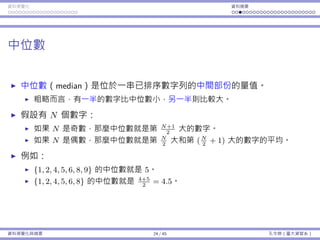
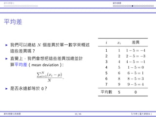
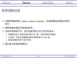
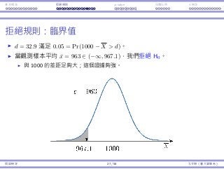
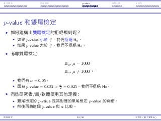
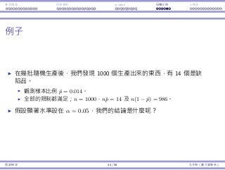
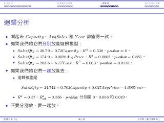
統計假設:例⼦三
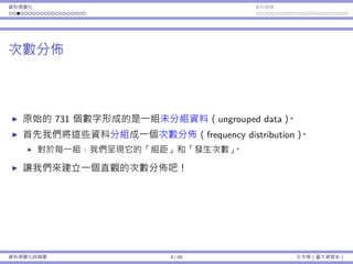
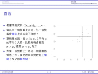
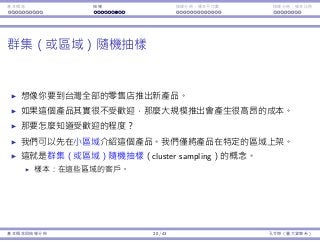
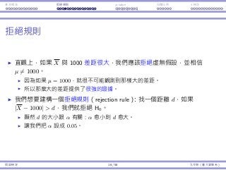
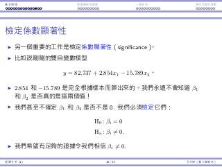
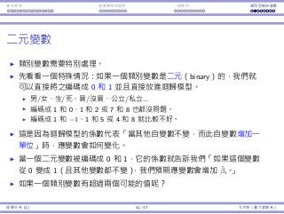
考慮以下假設:「這個候選⼈有超過 50% 選⺠的⽀持。」
我們需要⼀個預設立場,⽽我們在乎的百分比為 50%,因此我們選擇的
虛無假設為
H0 : p = 0.5。
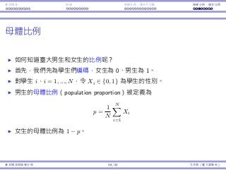
p 是偏好⽀持該候選⼈的選⺠⺟體比例。
更精確⽽⾔,令 Xi = 1 如果該選⺠ i 偏好⽀持這個候選⼈,否則以 0 表
⽰,i = 1, ..., N,那麼 p =
∑N
i=1 Xi
N
。
那對立假設呢?是
Ha : p 0.5 還是 Ha : p 0.5?
假設檢定 9 / 58 孔令傑(臺⼤資管系)
98.
基本概念 拒絕規則 p-value⺟體比例 t 檢定
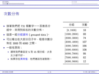
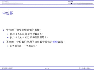
統計假設:例⼦三
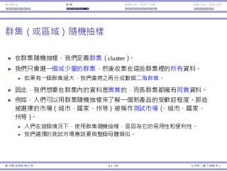
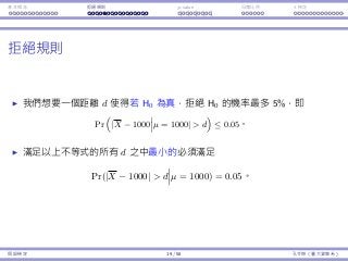
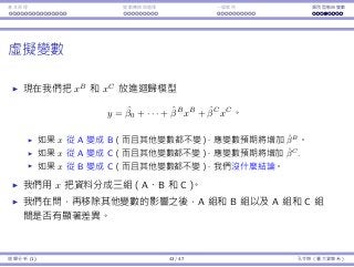
對立假設的選擇取決於要進⾏的決策或⾏動。
假設⼀個⼈只有在相信⾃⼰會贏的時候(即 p 0.5)才會參選,那麼
對立假設為
Ha : p 0.5。
假設⼀個⼈傾向參選,並只有在獲勝機率低時才會退出,則對立假設為
Ha : p 0.5。
對立假設是「我們想要(需要)證明的事」。
假設檢定 10 / 58 孔令傑(臺⼤資管系)
基本概念 拒絕規則 p-value⺟體比例 t 檢定
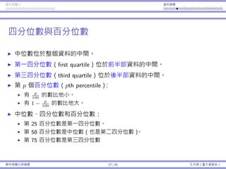
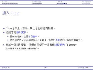
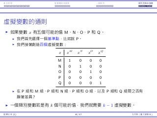
課程⼤綱
基本概念。
拒絕規則。
p-value。
⺟體比例。
t 檢定。
假設檢定 46 / 58 孔令傑(臺⼤資管系)
135.
基本概念 拒絕規則 p-value⺟體比例 t 檢定
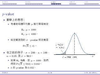
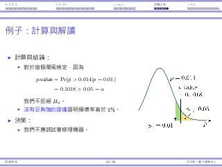
z 檢定
在例⼦⼀,基本上我們是⽤ X ∼ ND(µ, σ√
n
) 這件事實。
這隱含了 X−µ
σ/
√
n
∼ ND(0, 1),也就是所謂的標準常態分佈,或是 z 分佈。
因此,這個檢定被稱為 z 檢定。
這需要知道 σ。
假設檢定 47 / 58 孔令傑(臺⼤資管系)
136.
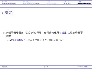
基本概念 拒絕規則 p-value⺟體比例 t 檢定
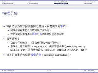
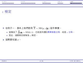
當變異數未知
當⺟體變異數 σ2
為未知, X−µ
σ/
√
n
的⼤⼩也就未知。
如果我們⽤樣本變異數 S2
作為替代呢?
定理 1
對於⼀個常態的⺟體,統計量
T =
X − µ
S/
√
n
從 t 分佈,且⾃由度為 n − 1。
什麼是 t 分佈?
假設檢定 48 / 58 孔令傑(臺⼤資管系)
137.
基本概念 拒絕規則 p-value⺟體比例 t 檢定
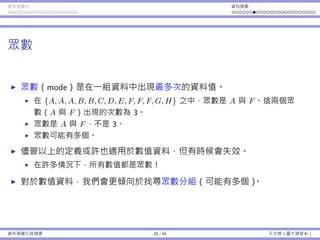
t 分佈
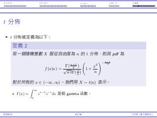
t 分佈被定義為以下:
定義 2
若⼀個隨機變數 X 從⾃由度為 n 的 t 分佈,則其 pdf 為
f(x|n) =
Γ(n+1
2 )
√
nπΓ(n
2 )
(
1 +
x2
n
)− n+1
2
對於所有的 x ∈ (−∞, ∞)。我們⽤ X ∼ t(n) 表⽰。
Γ(x) =
∫ ∞
0
zx−1
e−z
dz 是個 gamma 函數。
假設檢定 49 / 58 孔令傑(臺⼤資管系)
138.
基本概念 拒絕規則 p-value⺟體比例 t 檢定
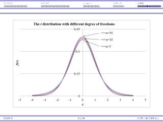
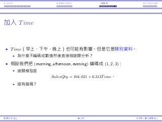
z 和 t 分佈
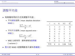
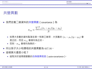
讓我們來比較 Z = X−µ
σ/
√
n
和 T = X−µ
S/
√
n
。
因為我們不知道 σ,我們⽤ S 來替代。
Z ∼ ND(0, 1) 且 T ∼ t(n − 1)。
因為 t 是 z 分佈的替代品,它也被設計為以 0 為中⼼:E[T] = E[Z] = 0。
但是,因為我們多加了⼀個隨機變數入算式(σ 是個已知的常數),T 會變
得比 Z「更隨機」,即 Var(T) Var(Z)。
圖形上,t 曲線會比 z 曲線更平。
當 n → ∞,t(n) → ND(0, 1)。
假設檢定 50 / 58 孔令傑(臺⼤資管系)
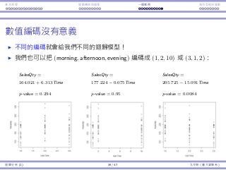
基本概念 拒絕規則 p-value⺟體比例 t 檢定
⼩結
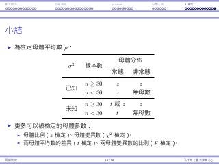
為檢定⺟體平均數 µ:
σ2
樣本數
⺟體分佈
常態 非常態
已知
n ≥ 30 z z
n 30 z 無⺟數
未知
n ≥ 30 t 或 z z
n 30 t 無⺟數
更多可以被檢定的⺟體參數:
⺟體比例(z 檢定)、⺟體變異數(χ2
檢定)。
兩⺟體平均數的差異(t 檢定)、兩⺟體變異數的比例(F 檢定)。
假設檢定 58 / 58 孔令傑(臺⼤資管系)
Interaction Endogeneity, residualsLogistic regression
Statistics and Data Analysis for Engineers
Part 4: Regression Analysis (2)
Ling-Chieh Kung
Department of Information Management
National Taiwan University
January 14, 2017
Regression Analysis (2) 1 / 38 Ling-Chieh Kung (NTU IM)
Interaction Endogeneity, residualsLogistic regression
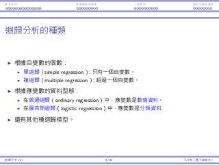
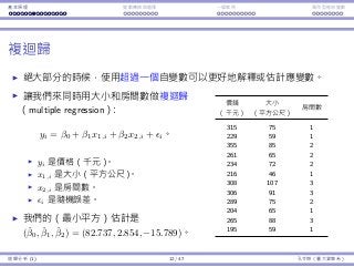
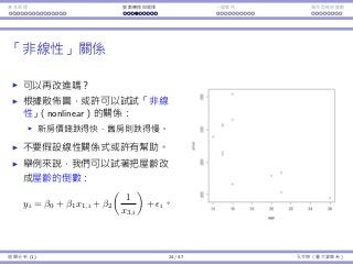
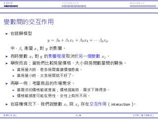
Interaction among variables
In a regression model
y = β0 + β1x1 + β2x2 + · · · βpxp,
βi measures how xi affects y.
Sometimes the impact of xi on y depends on the value of another
variable xj.
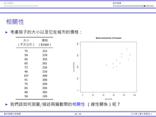
Consider house prices, sizes, and numbers of bedrooms.
When a house is big, more numbers of bedrooms may be good.
When a house is small, more numbers of bedrooms may be bad.
Consider the demand of a product.
Demand is sensitive to price: When price goes up, demand goes down.
The sensitivity may be different between men and women.
In this case, we say there is an interaction between xi and xj.
Regression Analysis (2) 3 / 38 Ling-Chieh Kung (NTU IM)
197.
Interaction Endogeneity, residualsLogistic regression
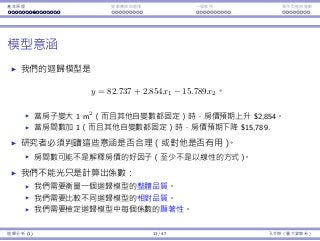
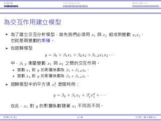
Modeling interaction
To model the interaction between xi and xj, one possibility is to create
a new variable xixj, which is the product of the two original variables.
In a regression model
y = β0 + β1x1 + β2x2 + β1,2x1x2 · · · ,
β1,2 measures the interaction between x1 and x2.
The impact of x1 on y is β1 + β1,2x2.
The impact of x2 on y is β2 + β1,2x1.
A quadratic term x2
i in a regression model
y = β0 + β1x1 + β1x2
1 + · · · ,
is a special case: The impact of x1 on y is depends on the value of x1.
Regression Analysis (2) 4 / 38 Ling-Chieh Kung (NTU IM)
198.
Interaction Endogeneity, residualsLogistic regression
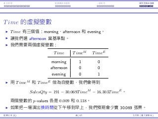
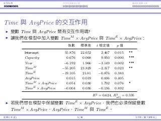
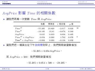
Interaction between Time and AvgPrice
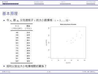
Do Time and AvgPrice affect each other’s impact?
Let’s add TimeM
× AvgPrice and TimeE
× AvgPrice into our model:
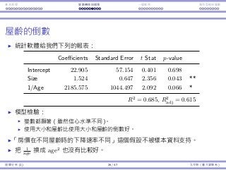
Coefficients Std. Error t Stat p-value
Intercept 55.876 22.652 2.467 0.015 **
Capacity 0.676 0.068 9.950 0.000 ***
Year −6.192 1.966 −3.149 0.002 ***
TimeM −55.205 23.829 −2.317 0.023 **
TimeE −19.105 21.81 −0.876 0.383
AvgPrice 0.015 0.019 0.836 0.405
TimeM × AvgPrice 0.054 0.030 1.792 0.076 *
TimeE × AvgPrice −0.004 0.030 −0.136 0.892
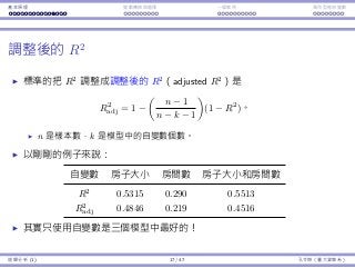
R2 = 0.624, R2
adj = 0.595
If we want to keep TimeE
× AvgPrice, we must also keep
TimeM
× AvgPrice, AvgPrice, TimeM
, and TimeE
in our model.
Regression Analysis (2) 5 / 38 Ling-Chieh Kung (NTU IM)
199.
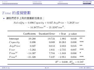
Interaction Endogeneity, residualsLogistic regression
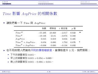
Time affects AvgPrice’s impact
Let’s focus on Time and AvgPrice:
Coefficients Std. Error t Stat p-value
TimeM −55.205 23.829 −2.317 0.023 **
TimeE −19.105 21.81 −0.876 0.383
AvgPrice 0.015 0.019 0.836 0.405
TimeM × AvgPrice 0.054 0.030 1.792 0.076 *
TimeE × AvgPrice −0.004 0.030 −0.136 0.892
People have different price sensitivity for shows at different time.
When the price goes up by $1, we expect:
The sales of an afternoon show increases by 0.015.
The sales of an morning show increases by 0.015 + 0.054 = 0.069.
The sales of a evening show increases by 0.015 − 0.004 = 0.011.
Regression Analysis (2) 6 / 38 Ling-Chieh Kung (NTU IM)
200.
Interaction Endogeneity, residualsLogistic regression
AvgPrice affects Time’s impact
Let’s focus on Time and AvgPrice:
Coefficients Std. Error t Stat p-value
TimeM −55.205 23.829 −2.317 0.023 **
TimeE −19.105 21.81 −0.876 0.383
AvgPrice 0.015 0.019 0.836 0.405
TimeM × AvgPrice 0.054 0.030 1.792 0.076 *
TimeE × AvgPrice −0.004 0.030 −0.136 0.892
If we reschedule an afternoon show to the morning, the impact is
−55.205 + 0.054AvgPrice
in expectation. If AvgPrice = 500, e.g., we expect the sales to decrease
by −55.205 + 0.054 × 500 = −28.205.
If we reschedule an afternoon show to the evening, the expected impact
is −19.105 − 0.004AvgPrice.
Regression Analysis (2) 7 / 38 Ling-Chieh Kung (NTU IM)
201.
Interaction Endogeneity, residualsLogistic regression
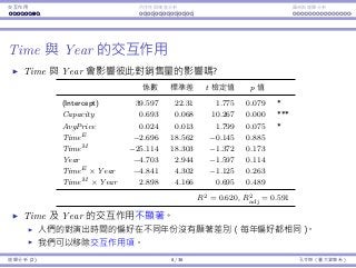
Interaction between Time affects Year
Do Time and Year affect each other’s impact?
Coefficients Std. Error t Stat p-value
(Intercept) 39.597 22.31 1.775 0.079 *
Capacity 0.693 0.068 10.267 0.000 ***
AvgPrice 0.024 0.013 1.799 0.075 *
TimeE −2.696 18.562 −0.145 0.885
TimeM −25.114 18.303 −1.372 0.173
Year −4.703 2.944 −1.597 0.114
TimeE × Year −4.841 4.302 −1.125 0.263
TimeM × Year 2.898 4.166 0.695 0.489
R2 = 0.620, R2
adj = 0.591
All the five variables related to Time and Year are insignificant.
People’s preference over the show time do not change from year to year.
The trend from year to year is the same for different show times.
Though all the five variables are insignificant, we typically first try to
remove only the interaction terms.
Regression Analysis (2) 8 / 38 Ling-Chieh Kung (NTU IM)
202.
Interaction Endogeneity, residualsLogistic regression
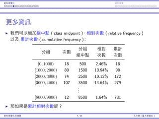
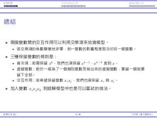
Summary
Two variables’ interaction may be modeled with a product term.
If its coefficient is significantly nonzero, one variable’s impact depends on
the other’s value.
Three rules for keeping variables:
Quadratic transformation: If we want to keep x2
, we must also keep x.
Indicator variable: If we want to keep xk
, where xk
is the indicator
variable for represent x = k , we must also keep xk
for all k = k .
Interaction: If we want to keep xixj, we must also keep xi and xj.
Therefore:
If we want to have xixk
j , where xk
j is the indicator variable for represent
xj = k , we must also keep xk
j for all k = k .
It is possible to add xixjxk into a regression model.
Regression Analysis (2) 9 / 38 Ling-Chieh Kung (NTU IM)
Interaction Endogeneity, residualsLogistic regression
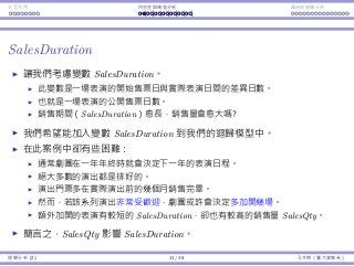
SalesDuration
Consider the variable SalesDuration.
The difference between the announce day and performance day.
The number of days that the tickets for a show are publicly sold.
The longer sales duration, the more sales?
We probably want to add SalesDuration into our regression model.
This is problematic in this case:
Typically the theater determines its schedule for the next year at the end
of each year.
Most performances are scheduled.
Ticket selling starts a few months before a series of shows are performed.
However, if a series turns out to be popular, the theater may decide to
add more shows into this series.
These additional shows have much shorter SalesDuration and typically
have high SalesQty.
In short, SalesQty affects SalesDuration.
Regression Analysis (2) 11 / 38 Ling-Chieh Kung (NTU IM)
205.
Interaction Endogeneity, residualsLogistic regression
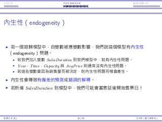
Endogeneity
If in a regression model an independent variable is affected by the
dependent variable, we say the model has the endogeneity problem.
If we add SalesDuration into our model, we creates endogeneity.
Year, Time, Capacity, and AvgPrice do not have the endogeneity
problem.
If any of them may be modified when the theater sees a good (or bad)
sales, endogeneity emerges.
Endogeneity results in a biased prediction.
In our ticket selling example, if we add SalesDuration into our model,
we may intentionally announce shows later!
Regression Analysis (2) 12 / 38 Ling-Chieh Kung (NTU IM)
206.
Interaction Endogeneity, residualsLogistic regression
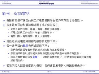
Example: promotional phone calls
A bank lets its workers call people to invite them to deposit money.
Many factors may affect the outcome (success or not):1
The callee’ gender, age, occupation, education level, etc.
The caller’s gender, age, experience, etc.
The calling day, calling time, weather at the call, etc.
All these information from past calls are recorded.
The length of each call is also recorded.
It is found to be highly correlated with success/failure.
However, it cannot be used as an independent variable.
Because it is affected by the outcome: Once one agrees to deposit
money, the call gets longer to talk about more details.
In this example, if we add call duration into our model, we may ask
our workers to speak as slowly as possible.
1A regression model that incorporates a qualitative dependent variable will be
introduced in later lectures.
Regression Analysis (2) 13 / 38 Ling-Chieh Kung (NTU IM)
207.
Interaction Endogeneity, residualsLogistic regression
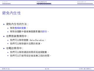
Avoiding endogeneity
To avoid endogeneity:
Remove the independent variable is endogenous.
Remove those records in which an independent variable is affected by
the dependent one.
In the ticket selling example:
We may remove SalesDuration.
We may remove those additional shows.
In the promotional call example:
We may remove the variable of call duration.
Regression Analysis (2) 14 / 38 Ling-Chieh Kung (NTU IM)
208.
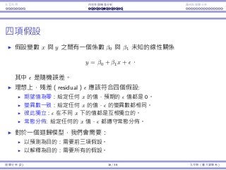
Interaction Endogeneity, residualsLogistic regression
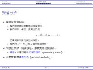
Residual analysis
When doing regression:
We try to discover the hidden relationship among variables.
We assume a specific model
y = β0 + β1x1 + · · · +
and then fit our sample data to the model.
We validate our model based on the degree of fitness (R2
and R2
adj)
and significance of variables (p-values).
If our model is good, the random error should be really “random.”
There should be no systematic pattern for .
We need residual analysis.
Regression Analysis (2) 15 / 38 Ling-Chieh Kung (NTU IM)
209.
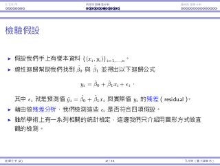
Interaction Endogeneity, residualsLogistic regression
Residuals
Consider a pair of variables x and y.
We may assume a linear relationship
y = β0 + β1x +
for some unknown parameters β0 and β1. is the random error.
Four assumptions on the random error:
Zero mean: The expected value of is zero for any value of x.
Constant variance: The variance of is the same for any value of x.
Independence: for different values of x should be independent.
Normality: is normal for any value of x.
Once we obtain a regression model, we need to test these assumptions.
To predict: We need the first three.
To explain: We need all the four.
Regression Analysis (2) 16 / 38 Ling-Chieh Kung (NTU IM)
210.
Interaction Endogeneity, residualsLogistic regression
Testing the four assumptions
Consider a sample data set {(xi, yi)}i=1,...,n.
Linear regression helps us find ˆβ0 and ˆβ1 based on the sample data and
obtain the regression formula
yi = ˆβ0 + ˆβ1xi + i,
in which the error term i is called the residual between our estimate
ˆyi = ˆβ0 + ˆβ1xi and the real value yi.
By conducting a residual analysis, we check these is to see if we
have the desired properties.
While there are rigorous statistical tests, we will only introduce some
graphical approaches.
Regression Analysis (2) 17 / 38 Ling-Chieh Kung (NTU IM)
211.
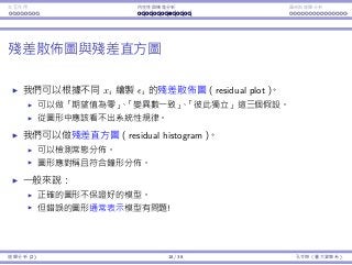
Interaction Endogeneity, residualsLogistic regression
The residual plot and histogram
We may plot the residuals is along with xis to form a residual plot.
This tests zero mean, constant variance, and independence.
There should be no systematic pattern.
We may construct a histogram of residuals.
This tests normality.
The histogram should be symmetric and bell-shaped.
In general:
A “good” plot does not guarantee a good model.
A “bad” plot strongly suggests that the model is bad!
Regression Analysis (2) 18 / 38 Ling-Chieh Kung (NTU IM)
212.
Interaction Endogeneity, residualsLogistic regression
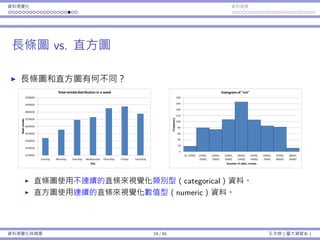
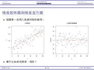
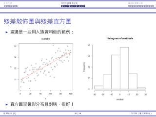
The residual plot and histogram
Consider the artificial data set as an example.
There is no pattern in the residual plot: good!
Regression Analysis (2) 19 / 38 Ling-Chieh Kung (NTU IM)
213.
Interaction Endogeneity, residualsLogistic regression
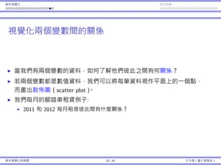
The residual plot and histogram
Consider the artificial data set as an example.
The histogram is symmetric and bell-shaped: good!
Regression Analysis (2) 20 / 38 Ling-Chieh Kung (NTU IM)
214.
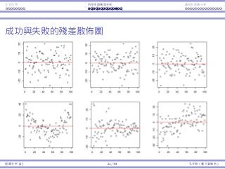
Interaction Endogeneity, residualsLogistic regression
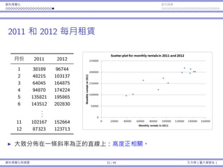
Residual plots that pass and fail the tests
Regression Analysis (2) 21 / 38 Ling-Chieh Kung (NTU IM)
215.
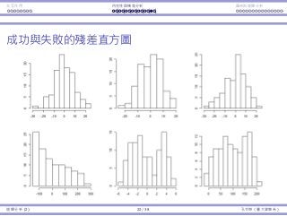
Interaction Endogeneity, residualsLogistic regression
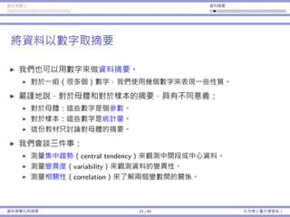
Histograms that pass and fail the tests
Regression Analysis (2) 22 / 38 Ling-Chieh Kung (NTU IM)
216.
Interaction Endogeneity, residualsLogistic regression
Residual analysis for multiple regression
Suppose that we construct a multiple regression model
yi = ˆβ0 + ˆβ1xi + · · · + ˆβpxp + i.
We still use residual plots and a histogram to test the assumptions.
Multiple residual plots should be depicted.
The vertical axis is always for the residuals is.
The horizontal axis is for a function of (x1, x2, ..., xp).
E.g., the kth independent variable xk along.
E.g., the fitted value ˆyi = ˆβ0 + ˆβ1xi + · · · + ˆβpxp.
Regression Analysis (2) 23 / 38 Ling-Chieh Kung (NTU IM)
Interaction Endogeneity, residualsLogistic regression
Logistic regression
So far our regression models always have a quantitative variable as
the dependent variable.
Some people call this type of regression ordinary regression.
To have a qualitative variable as the dependent variable, ordinary
regression does not work.
One popular remedy is to use logistic regression.
In general, a logistic regression model allows the dependent variable to
have multiple levels.
We will only consider binary variables in this lecture.
Let’s first illustrate why ordinary regression fails when the dependent
variable is binary.
Regression Analysis (2) 25 / 38 Ling-Chieh Kung (NTU IM)
219.
Interaction Endogeneity, residualsLogistic regression
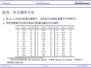
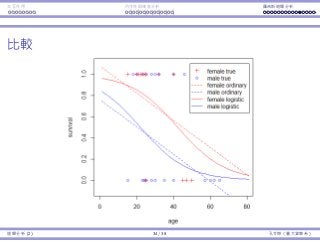
Example: survival probability
45 persons got trapped in a storm during a mountain hiking.
Unfortunately, some of them died due to the storm.2
We want to study how the survival probability of a person is
affected by her/his gender and age.
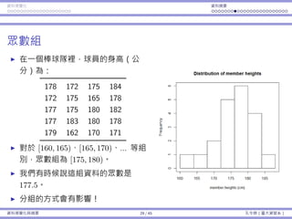
Age Gender Survived Age Gender Survived Age Gender Survived
23 Male No 23 Female Yes 15 Male No
40 Female Yes 28 Male Yes 50 Female No
40 Male Yes 15 Female Yes 21 Female Yes
30 Male No 47 Female No 25 Male No
28 Male No 57 Male No 46 Male Yes
40 Male No 20 Female Yes 32 Female Yes
45 Female No 18 Male Yes 30 Male No
62 Male No 25 Male No 25 Male No
65 Male No 60 Male No 25 Male No
45 Female No 25 Male Yes 25 Male No
25 Female No 20 Male Yes 30 Male No
28 Male Yes 32 Male Yes 35 Male No
28 Male No 32 Female Yes 23 Male Yes
23 Male No 24 Female Yes 24 Male No
22 Female Yes 30 Male Yes 25 Female Yes
2The data set comes from the textbook The Statistical Sleuth by Ramsey and
Schafer. The story has been modified.
Regression Analysis (2) 26 / 38 Ling-Chieh Kung (NTU IM)
220.
Interaction Endogeneity, residualsLogistic regression
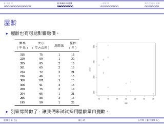
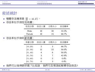
Descriptive statistics
Overall survival probability is 20
45 = 44.4%.
Survival or not seems to be affected by gender.
Group Survivals Group size Survival probability
Male 10 30 33.3%
Female 10 15 66.7%
Survival or not seems to be affected by age.
Age class Survivals Group size Survival probability
[10, 20) 2 3 66.7%
[21, 30) 11 22 50.0%
[31, 40) 4 8 50.0%
[41, 50) 3 7 42.9%
[51, 60) 0 2 0.0%
[61, 70) 0 3 0.0%
May we do better? May we predict one’s survival probability?
Regression Analysis (2) 27 / 38 Ling-Chieh Kung (NTU IM)
221.
Interaction Endogeneity, residualsLogistic regression
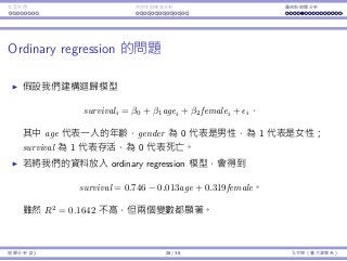
Ordinary regression is problematic
Immediately we may want to construct a linear regression model
survivali = β0 + β1agei + β2femalei + i.
where age is one’s age, gender is 0 if the person is a male or 1 if
female, and survival is 1 if the person is survived or 0 if dead.
By conducting ordinary regression, we may obtain the regression line
survival = 0.746 − 0.013age + 0.319female.
Though R2
= 0.1642 is low, both variables are significant.
Regression Analysis (2) 28 / 38 Ling-Chieh Kung (NTU IM)
222.
Interaction Endogeneity, residualsLogistic regression
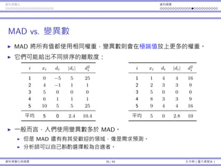
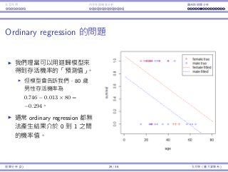
Ordinary regression is problematic
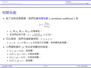
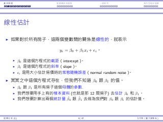
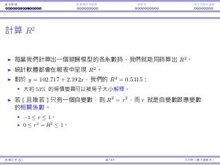
The regression model gives
us “predicted survival
probability.”
For a man at 80, the
“probability” becomes
0.746−0.013×80 = −0.294,
which is unrealistic.
In general, it is very easy for
an ordinary regression
model to generate predicted
“probability” not within 0
and 1.
Regression Analysis (2) 29 / 38 Ling-Chieh Kung (NTU IM)
223.
Interaction Endogeneity, residualsLogistic regression
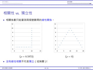
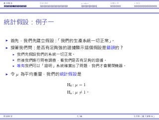
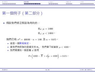
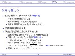
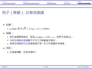
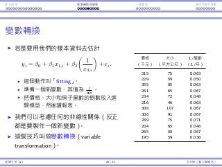
Logistic regression
The right way to do is to do logistic regression.
Consider the age-survival example.
We still believe that the smaller age increases the survival probability.
However, not in a linear way.
It should be that when one is young enough, being younger does not
help too much.
The marginal benefit of being younger should be decreasing.
The marginal loss of being older should also be decreasing.
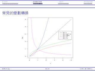
One particular functional form that exhibits this
property is
y =
ex
1 + ex
⇔ log
y
1 − y
= x
x can be anything in (−∞, ∞).
y is limited in [0, 1].
Regression Analysis (2) 30 / 38 Ling-Chieh Kung (NTU IM)
224.
Interaction Endogeneity, residualsLogistic regression
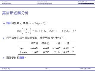
Logistic regression
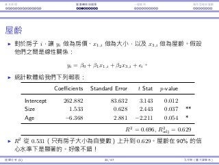
We hypothesize that independent variables xis affect π, the
probability for y to be 1, in the following form:3
log
π
1 − π
= β0 + β1x1 + β2x2 + · · · + βpxp.
By conducting logistic regression, we obtain the regression report.
Some information is new, but the following is familiar:
Estimate Std. Error z value p-value
age −0.078 0.037 −2.097 0.036 *
female 1.597 0.755 2.114 0.035 *
Both variables are significant.
3Numerical algorithms are used to search for coefficients to make the curve fit
the given data points in the best way.
Regression Analysis (2) 31 / 38 Ling-Chieh Kung (NTU IM)
225.
Interaction Endogeneity, residualsLogistic regression
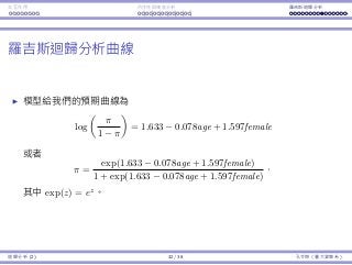
The Logistic regression curve
The estimated curve is
log
π
1 − π
= 1.633 − 0.078age + 1.597female,
or equivalently,
π =
exp(1.633 − 0.078age + 1.597female)
1 + exp(1.633 − 0.078age + 1.597female)
,
where exp(z) means ez
for all z ∈ R.
Regression Analysis (2) 32 / 38 Ling-Chieh Kung (NTU IM)
226.
Interaction Endogeneity, residualsLogistic regression
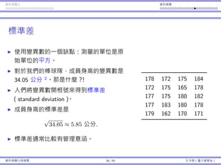
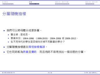
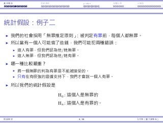
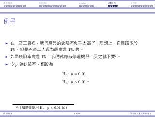
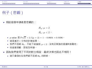
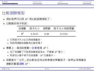
The Logistic regression curve
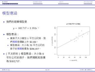
The curves can be used to
do prediction.
For a man at 80, π is
exp(1.633−0.078×80)
1+exp(1.633−0.078×80) ,
which is 0.0097.
For a woman at 60, π is
exp(1.633−0.078×60+1.597)
1+exp(1.633−0.078×60+1.597) ,
which is 0.1882.
π is always in [0, 1]. There is
no problem for interpreting
π as a probability.
Regression Analysis (2) 33 / 38 Ling-Chieh Kung (NTU IM)
Interaction Endogeneity, residualsLogistic regression
Interpretations
The estimated curve is
log
π
1 − π
= 1.633 − 0.078age + 1.597female.
Any implication?
−0.078age: Younger people will survive more likely.
1.597female: Women will survive more likely.
In general:
Use the p-values to determine the significance of variables.
Use the signs of coefficients to give qualitative implications.
Use the formula to make predictions.
Regression Analysis (2) 35 / 38 Ling-Chieh Kung (NTU IM)
229.
Interaction Endogeneity, residualsLogistic regression
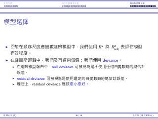
Model selection
Recall that in ordinary regression, we use R2
and adjusted R2
to assess
the usefulness of a model.
In logistic regression, we do not have R2
and adjusted R2
.
We have deviance instead.
In a regression report, the null deviance can be considered as the total
estimation errors without using any independent variable.
The residual deviance can be considered as the total estimation errors
by using the selected independent variables.
Ideally, the residual deviance should be small.4
4To be more rigorous, the residual deviance should also be close to its degree of
freedom. This is beyond the scope of this course.
Regression Analysis (2) 36 / 38 Ling-Chieh Kung (NTU IM)
230.
Interaction Endogeneity, residualsLogistic regression
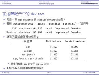
Deviances in the regression report
The null and residual deviances are provided in the regression report.
For glm(d$survival ~ d$age + d$female, binomial), we have
Null deviance: 61.827 on 44 degrees of freedom
Residual deviance: 51.256 on 42 degrees of freedom
Let’s try some models:
Independent variable(s) Null deviance Residual deviance
age 61.827 56.291
female 61.827 57.286
age, female 61.827 51.256
age, female, age × female 61.827 47.346
Using age only is better than using female only.
How to compare models with different numbers of variables?
Regression Analysis (2) 37 / 38 Ling-Chieh Kung (NTU IM)
231.
Interaction Endogeneity, residualsLogistic regression
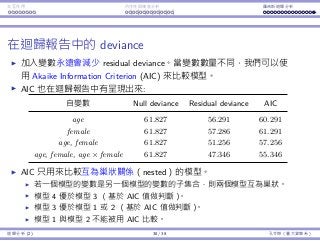
Deviances in the regression report
Adding variables will always reduce the residual deviance.
To take the number of variables into consideration, we may use
Akaike Information Criterion (AIC).
AIC is also included in the regression report:
Independent variable(s) Null deviance Residual deviance AIC
age 61.827 56.291 60.291
female 61.827 57.286 61.291
age, female 61.827 51.256 57.256
age, female, age × female 61.827 47.346 55.346
AIC is only used to compare nested models.
Two models are nested if one’s variables are form a subset of the other’s.
Model 4 is better than model 3 (based on their AICs).
Model 3 is better than either model 1 or model 2 (based on their AICs).
Model 1 and 2 cannot be compared (based on their AICs).
Regression Analysis (2) 38 / 38 Ling-Chieh Kung (NTU IM)


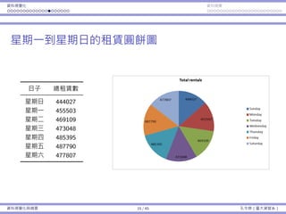
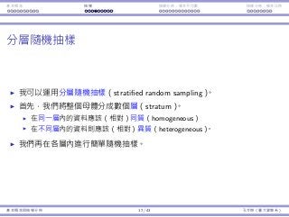
![資料視覺化 資料摘要
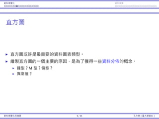
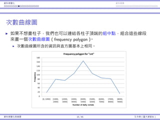
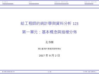
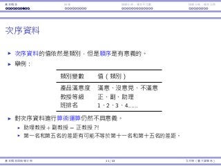
次數分佈
⼀種分組⽅式:
編號 分組 代表意義
1 [0, 1000) 0 ≤ x < 1000
2 [1000, 2000) 1000 ≤ x < 2000
3 [2000, 3000) 2000 ≤ x < 3000
...
8 [7000, 8000) 7000 ≤ x < 8000
9 [8000, 9000) 8000 ≤ x < 9000
有無限多種分組⽅式;通常各組組距會等⻑。
各分組之間應該要沒有空隙:[0, 999]、[1000, 1999]、... 是錯的。
各分組織間應該要不重疊:[0, 1000]、[1000, 1999]、... 是錯的。
資料視覺化與摘要 5 / 45 孔令傑(臺⼤資管系)](https://image.slidesharecdn.com/0114lckungtdsaprerequisite-170110090917/85/123-5-320.jpg)


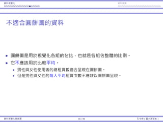


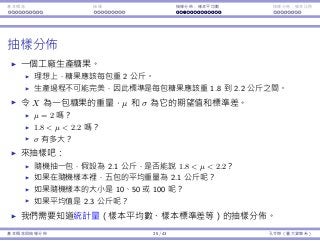
![基本概念 抽樣 抽樣分佈:樣本平均數 抽樣分佈:樣本比例
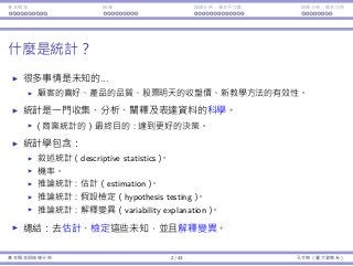
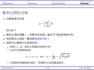
樣本平均的平均和變異數
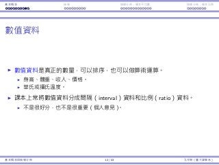
這些名詞是否使你困惑?
樣本平均數 vs. 樣本平均數的平均數。
樣本變異數 vs. 樣本平均數的變異數。
就定義⽽⾔,它們:
¯x = 1
n
∑n
i=1 Xi;⼀個隨機變數。
µ¯x = E[¯x];⼀個常數項。
s2
= 1
n−1
∑n
i=1(Xi − ¯x)2
;⼀個隨機變數。
σ2
¯x = Var(¯x);⼀個常數項。
樣本變異數也有它⾃⼰的平均和變異數。
基本概念與抽樣分佈 28 / 43 孔令傑(臺⼤資管系)](https://image.slidesharecdn.com/0114lckungtdsaprerequisite-170110090917/85/123-73-320.jpg)
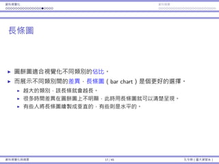
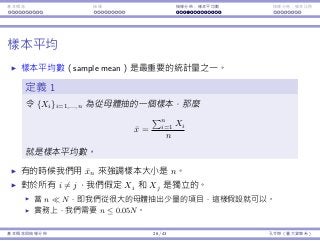
![基本概念 抽樣 抽樣分佈:樣本平均數 抽樣分佈:樣本比例
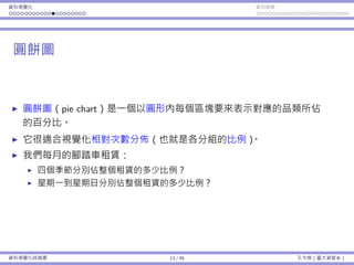
例⼦:品質檢驗
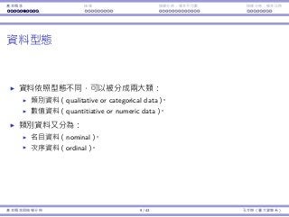
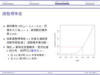
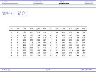
每包糖果的重量服從常態分佈,平均數為 µ = 2,標準差為 σ = 0.2。
假設品管⻑官決定要抽四包糖果並計算樣本平均 ¯x。如果 ¯x /∈ [1.8, 2.2],
我就會受罰。
我的⽣產流程其實是「好的」:µ = 2。
不幸地,它不是完美:σ > 0。
我們可能還是會被懲罰(如果運氣不好),儘管 µ = 2。
有多少的機率我會被懲罰呢?
我們想要計算 1 − Pr(1.8 < ¯x < 2.2)。
我們知道 µ¯x = µ = 2 且 σ¯x = σ√
4
= 0.1。
但我們並不知道 ¯x 的機率分佈!
基本概念與抽樣分佈 29 / 43 孔令傑(臺⼤資管系)](https://image.slidesharecdn.com/0114lckungtdsaprerequisite-170110090917/85/123-74-320.jpg)
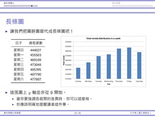
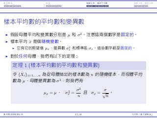
![基本概念 抽樣 抽樣分佈:樣本平均數 抽樣分佈:樣本比例
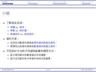
再回到這個例⼦:品質檢驗
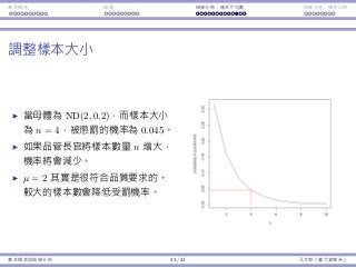
每包糖果的重量服從常態分佈,平均數為 µ = 2,標準差為 σ = 0.2。
假設品管⻑官決定要抽四包糖果並計算樣本平均 ¯x。如果 ¯x /∈ [1.8, 2.2],
我就會受罰。
有多少的機率我會被懲罰呢?
樣本平均數 ¯x 的分佈為 ND(2, 0.1)。
受罰機率 Pr(¯x < 1.8) + Pr(¯x > 2.2) ≈ 0.045。
基本概念與抽樣分佈 31 / 43 孔令傑(臺⼤資管系)](https://image.slidesharecdn.com/0114lckungtdsaprerequisite-170110090917/85/123-76-320.jpg)


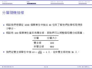
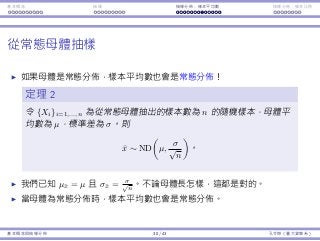
![基本概念 拒絕規則 p-value ⺟體比例 t 檢定
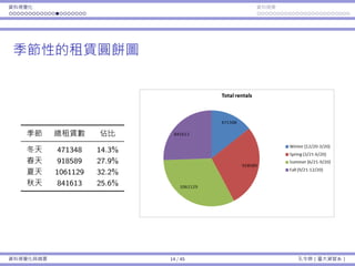
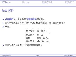
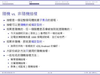
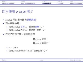
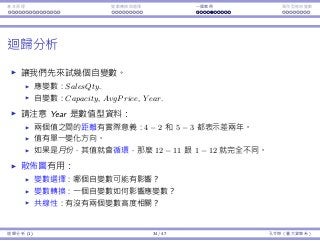
使⽤ p-value 的好處
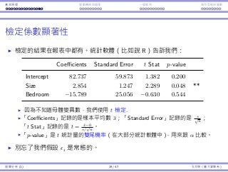
在很多的研究中,研究者在進⾏檢定之前,不會決定顯著⽔準 α。
他們計算 p-value,然後以星號標記結果的顯著性 。
⼀個典型給予星號的⽅式:
p-value 顯著 標記
(0, 0.01] ⾼度顯著 ***
(0.01, 0.05] 中等顯著 **
(0.05, 0.1] 輕微顯著 *
(0.1, 1) 不顯著 (Empty)
假設檢定 36 / 58 孔令傑(臺⼤資管系)](https://image.slidesharecdn.com/0114lckungtdsaprerequisite-170110090917/85/123-124-320.jpg)


![基本概念 拒絕規則 p-value ⺟體比例 t 檢定
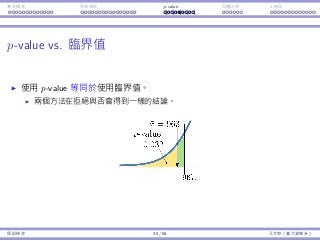
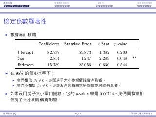
z 和 t 分佈
讓我們來比較 Z = X−µ
σ/
√
n
和 T = X−µ
S/
√
n
。
因為我們不知道 σ,我們⽤ S 來替代。
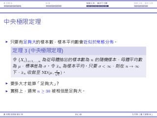
Z ∼ ND(0, 1) 且 T ∼ t(n − 1)。
因為 t 是 z 分佈的替代品,它也被設計為以 0 為中⼼:E[T] = E[Z] = 0。
但是,因為我們多加了⼀個隨機變數入算式(σ 是個已知的常數),T 會變
得比 Z「更隨機」,即 Var(T) Var(Z)。
圖形上,t 曲線會比 z 曲線更平。
當 n → ∞,t(n) → ND(0, 1)。
假設檢定 50 / 58 孔令傑(臺⼤資管系)](https://image.slidesharecdn.com/0114lckungtdsaprerequisite-170110090917/85/123-138-320.jpg)


![基本原理 變數轉換與選擇 ⼀個案例 類別型態⾃變數
線性估計
給定我們⽤樣本資料算出的 ˆβ0 和 ˆβ1,我們就會⽤ ˆyi = ˆβ0 + ˆβ1xi 來做
為我們對 yi 的估計值。
我們希望我們的估計誤差(estimation error)ϵi = yi − ˆyi 愈⼩愈好。
把所有誤差 ϵi 集合起來,我們希望總平⽅誤差(sum of squared errors,
SSE)愈⼩愈好:
n∑
i=1
ϵ2
i = (yi − ˆyi)2
=
n∑
i=1
[
(yi − (ˆβ0 + ˆβ1xi)
]2
。
我們求解(給定樣本資料後的)
min
ˆβ0, ˆβ1
n∑
i=1
[
(yi − (ˆβ0 + ˆβ1xi)
]2
最⼩平⽅估計(least square approximation)問題。
迴歸分析 (1) 9 / 47 孔令傑(臺⼤資管系)](https://image.slidesharecdn.com/0114lckungtdsaprerequisite-170110090917/85/123-155-320.jpg)
![基本原理 變數轉換與選擇 ⼀個案例 類別型態⾃變數
最⼩平⽅估計
最⼩平⽅估計問題
min
ˆβ0, ˆβ1
n∑
i=1
[
(yi − (ˆβ0 + ˆβ1xi)
]2
的最佳 (ˆβ0, ˆβ1) 是有公式解的:
ˆβ1 =
∑n
i=1(xi − ¯x)(yi − ¯y)
∑n
i=1(xi − ¯x)2
和 ˆβ0 = ¯y − ˆβ1 ¯x。
根據我們的 12 間房⼦,我們會得到 (ˆβ0, ˆβ1) = (102.717, 2.192).
這組樣本的 SSE 是 13118.63.
我們永遠不知道真正的 β0 和 β1。不過,根據我們的樣本資料,我們「最佳
的」猜想是 β0 = 102.717 和 β1 = 2.192。
迴歸分析 (1) 10 / 47 孔令傑(臺⼤資管系)](https://image.slidesharecdn.com/0114lckungtdsaprerequisite-170110090917/85/123-156-320.jpg)
![基本原理 變數轉換與選擇 ⼀個案例 類別型態⾃變數
模型檢驗:整體品質
如何衡量⼀個迴歸模型 y = ˆβ0 + ˆβ1x1 + · · · ˆβkxk 的品質?
如果完全不使⽤任何⾃變數,我們會⽤ ¯y =
∑n
i=1 yi
n 估計 yi。此時最⼤
平⽅誤差(sum of squared total errors,SST)是 SST =
∑n
i=1(yi − ¯y)2
。
根據我們的迴歸模型,我們把誤差降到
SSE =
n∑
i=1
(yi − ˆyi)2
=
n∑
i=1
[
(yi − (ˆβ0 + ˆβ1xi)
]2
。
⾃變數的變異中,能被我們的迴歸模型解釋的比例是
0 ≤ R2
= 1 −
SSE
SST
≤ 1。
R2
愈⼤,迴歸模型愈好。
迴歸分析 (1) 14 / 47 孔令傑(臺⼤資管系)](https://image.slidesharecdn.com/0114lckungtdsaprerequisite-170110090917/85/123-160-320.jpg)


![Interaction Endogeneity, residuals Logistic regression
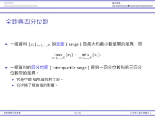
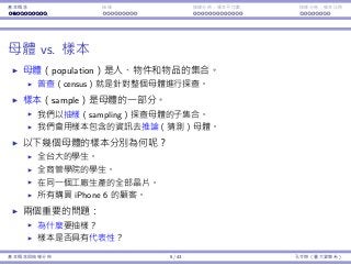
Logistic regression
The right way to do is to do logistic regression.
Consider the age-survival example.
We still believe that the smaller age increases the survival probability.
However, not in a linear way.
It should be that when one is young enough, being younger does not
help too much.
The marginal benefit of being younger should be decreasing.
The marginal loss of being older should also be decreasing.
One particular functional form that exhibits this
property is
y =
ex
1 + ex
⇔ log
y
1 − y
= x
x can be anything in (−∞, ∞).
y is limited in [0, 1].
Regression Analysis (2) 30 / 38 Ling-Chieh Kung (NTU IM)](https://image.slidesharecdn.com/0114lckungtdsaprerequisite-170110090917/85/123-223-320.jpg)
![Interaction Endogeneity, residuals Logistic regression
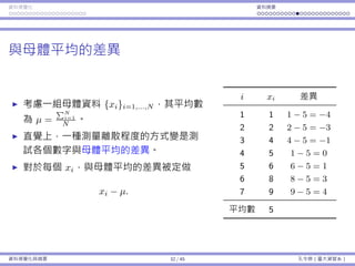
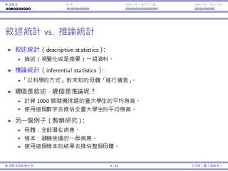
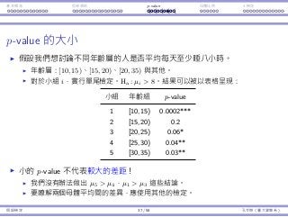
The Logistic regression curve
The curves can be used to
do prediction.
For a man at 80, π is
exp(1.633−0.078×80)
1+exp(1.633−0.078×80) ,
which is 0.0097.
For a woman at 60, π is
exp(1.633−0.078×60+1.597)
1+exp(1.633−0.078×60+1.597) ,
which is 0.1882.
π is always in [0, 1]. There is
no problem for interpreting
π as a probability.
Regression Analysis (2) 33 / 38 Ling-Chieh Kung (NTU IM)](https://image.slidesharecdn.com/0114lckungtdsaprerequisite-170110090917/85/123-226-320.jpg)


![[DL輪読会]Bayesian Uncertainty Estimation for Batch Normalized Deep Networks](https://cdn.slidesharecdn.com/ss_thumbnails/190719dlver2-190719035734-thumbnail.jpg?width=640&height=640&fit=bounds)


![[台灣人工智慧學校] 工業 4.0 與智慧製造的發展趨勢與挑戰](https://cdn.slidesharecdn.com/ss_thumbnails/20190316jyh-horngchou-190315170336-thumbnail.jpg?width=640&height=640&fit=bounds)


![[DL輪読会]Model soups: averaging weights of multiple fine-tuned models improves ...](https://cdn.slidesharecdn.com/ss_thumbnails/dl0401-220405031053-thumbnail.jpg?width=640&height=640&fit=bounds)


![[系列活動] Machine Learning 機器學習課程](https://cdn.slidesharecdn.com/ss_thumbnails/ml4ds02122017-170212005829-thumbnail.jpg?width=640&height=640&fit=bounds)
![[系列活動] 智慧製造與生產線上的資料科學 (製造資料科學:從預測性思維到處方性決策)](https://cdn.slidesharecdn.com/ss_thumbnails/20170211datascienceinmanufacturing-170205150525-thumbnail.jpg?width=640&height=640&fit=bounds)
![[系列活動] 無所不在的自然語言處理—基礎概念、技術與工具介紹](https://cdn.slidesharecdn.com/ss_thumbnails/nlptutorial-0828-170830062001-thumbnail.jpg?width=640&height=640&fit=bounds)

![[DSC 2016] 系列活動:李泳泉 / 星火燎原 - Spark 機器學習初探](https://cdn.slidesharecdn.com/ss_thumbnails/sparkmllib-161026052038-thumbnail.jpg?width=640&height=640&fit=bounds)
![[系列活動] 資料探勘速遊 - Session4 case-studies](https://cdn.slidesharecdn.com/ss_thumbnails/session4-case-studies-170114072124-thumbnail.jpg?width=640&height=640&fit=bounds)


![[系列活動] 手把手教你R語言資料分析實務](https://cdn.slidesharecdn.com/ss_thumbnails/stepbystepr20170114-170113030702-thumbnail.jpg?width=640&height=640&fit=bounds)

![[系列活動] Data exploration with modern R](https://cdn.slidesharecdn.com/ss_thumbnails/dataexplorationwithmodernr1221-161219044516-thumbnail.jpg?width=640&height=640&fit=bounds)
![[系列活動] Python 程式語言起步走](https://cdn.slidesharecdn.com/ss_thumbnails/python20170812-170808043244-thumbnail.jpg?width=640&height=640&fit=bounds)
![[系列活動] 機器學習速遊](https://cdn.slidesharecdn.com/ss_thumbnails/mltourhandout-170310083857-thumbnail.jpg?width=640&height=640&fit=bounds)


![[台灣人工智慧學校] 人工智慧技術發展與應用](https://cdn.slidesharecdn.com/ss_thumbnails/version5-final-190319060225-thumbnail.jpg?width=640&height=640&fit=bounds)
![[台灣人工智慧學校] 執行長報告](https://cdn.slidesharecdn.com/ss_thumbnails/openingsw-190315170512-thumbnail.jpg?width=640&height=640&fit=bounds)
![[台灣人工智慧學校] 開創台灣產業智慧轉型的新契機](https://cdn.slidesharecdn.com/ss_thumbnails/aiotforaiabytedchangho-190227081005-thumbnail.jpg?width=640&height=640&fit=bounds)
![[台灣人工智慧學校] 開創台灣產業智慧轉型的新契機](https://cdn.slidesharecdn.com/ss_thumbnails/aiinhealthcare-20190216victoria-v6-190227081004-thumbnail.jpg?width=640&height=640&fit=bounds)
![[台灣人工智慧學校] 台北總校第三期結業典禮 - 執行長談話](https://cdn.slidesharecdn.com/ss_thumbnails/tp3closingsw-190126030359-thumbnail.jpg?width=640&height=640&fit=bounds)
![[TOxAIA台中分校] AI 引爆新工業革命,智慧機械首都台中轉型論壇](https://cdn.slidesharecdn.com/ss_thumbnails/aia-chen-190116063635-thumbnail.jpg?width=640&height=640&fit=bounds)
![[TOxAIA台中分校] 2019 台灣數位轉型 與產業升級趨勢觀察](https://cdn.slidesharecdn.com/ss_thumbnails/to-sheng-190116063620-thumbnail.jpg?width=640&height=640&fit=bounds)
![[TOxAIA台中分校] 智慧製造成真! 產線導入AI的致勝關鍵](https://cdn.slidesharecdn.com/ss_thumbnails/thu-hsu-190116063619-thumbnail.jpg?width=640&height=640&fit=bounds)
![[台灣人工智慧學校] 從經濟學看人工智慧產業應用](https://cdn.slidesharecdn.com/ss_thumbnails/1-the-application-of-ai-industry-from-economics-190108064940-thumbnail.jpg?width=640&height=640&fit=bounds)
![[台灣人工智慧學校] 台中分校第二期開學典禮 - 執行長報告](https://cdn.slidesharecdn.com/ss_thumbnails/tc2-opening1-compressed-190107034100-thumbnail.jpg?width=640&height=640&fit=bounds)

![[台中分校] 第一期結業典禮 - 執行長談話](https://cdn.slidesharecdn.com/ss_thumbnails/sw-ppt-181217031715-thumbnail.jpg?width=640&height=640&fit=bounds)
![[TOxAIA新竹分校] 工業4.0潛力新應用! 多模式對話機器人](https://cdn.slidesharecdn.com/ss_thumbnails/20181206004-181210031031-thumbnail.jpg?width=640&height=640&fit=bounds)
![[TOxAIA新竹分校] AI整合是重點! 竹科的關鍵轉型思維](https://cdn.slidesharecdn.com/ss_thumbnails/20181206002-181210031031-thumbnail.jpg?width=640&height=640&fit=bounds)
![[TOxAIA新竹分校] 2019 台灣數位轉型與產業升級趨勢觀察](https://cdn.slidesharecdn.com/ss_thumbnails/20181206-001-181210031002-thumbnail.jpg?width=640&height=640&fit=bounds)
![[TOxAIA新竹分校] 深度學習與Kaggle實戰](https://cdn.slidesharecdn.com/ss_thumbnails/20181206003-181210031001-thumbnail.jpg?width=640&height=640&fit=bounds)
![[台灣人工智慧學校] Bridging AI to Precision Agriculture through IoT](https://cdn.slidesharecdn.com/ss_thumbnails/hc-2nd-openingai-school-181206104858-thumbnail.jpg?width=640&height=640&fit=bounds)
![[2018 台灣人工智慧學校校友年會] 產業經驗分享: 如何用最少的訓練樣本,得到最好的深度學習影像分析結果,減少一半人力,提升一倍品質 / 李明達](https://cdn.slidesharecdn.com/ss_thumbnails/lee-181130104127-thumbnail.jpg?width=640&height=640&fit=bounds)
![[2018 台灣人工智慧學校校友年會] 啟動物聯網新關鍵 - 未來由你「喚」醒 / 沈品勳](https://cdn.slidesharecdn.com/ss_thumbnails/20181117shengfn-181130083931-thumbnail.jpg?width=640&height=640&fit=bounds)
![[2018 台灣人工智慧學校校友年會] Practical experience in mining and evaluating information...](https://cdn.slidesharecdn.com/ss_thumbnails/1615-1655chenaia-info-sys-exp-181130083557-thumbnail.jpg?width=640&height=640&fit=bounds)