AN EXCLUSIVE PPT ON REMOTE SENSING IIRS

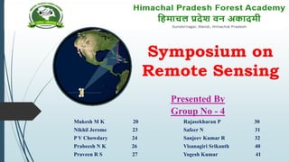
1. Symposium on
Remote Sensing
Presented By
Group No - 4
Mukesh M K 20 Rajasekharan P 30
Nikhil Jerome 23 Safeer N 31
P V Chowdary 24 Sanjeev Kumar R 32
Prabeesh N K 26 Visanagiri Srikanth 40
Praveen R S 27 Yogesh Kumar 41

2. Topic Covered

4.  Mapping and Monitoring of forest cover type using Remote Sensing is a
systematic understanding of the forest map development and to map the
existing forest coverage in context of cost effectiveness and time consumption.
 Mapping and Monitoring of forest cover type using Remote Sensing requires
reliable inventory data and the maps indicating current state of the forest area.
 The advantages of Remote Sensing, Geographic Information System and
Global Positioning System technologies has revolutionized the forest resource
assessment, monitoring management and has reduced the tome and cost
considerably.
INTRODUCTION

5. DEFINITIONS
 Forest Type: A unit of vegetation that possess broad characteristics in
physiognomy and structure sufficiently pronounced to permit its
differentiation from other such units.
 It signifies natural floral biodiversity, important consideration for
silvicultural prescriptions, an appropriate basis for stratification of
forests, facilitates valuation of forest, basis for carbon assessment
(REDD), Important consideration in impact studies, important input in
management and working plans, application in climate change studies.

7. SPATIAL DATA BASE AND ITS SOURCES
 Suitable GIS software and supporting
system.
 Spatial database layers on different themes,
attribute data in attribute table.
 On screen digitization for creating various
layers on 1:25000 or higher
 A common projection parameters: Projection
system UTM, Datum: Spheroid – WGS
84/Everest.
 Satellite images with spatial resolution of 5.8
Meter or higher only.
 Attribute of forest area in attribute table
should be as per Government records.
 Land cover map at Division level at 1:50000
scale.
 Forest types map available in FSI/Maps
available with Department.
 Forest density available with FSI/Self
interpretation.

9. CHOICE OF SEASON OF SATELLITE DATA
VEGETATION ZONE PROPER SEASON
Humid and moist evergreen and semi evergreen vegetation
in western and eastern Ghats
January –February
Humid and moist evergreen and semi evergreen vegetation
North Eastern Region
February – March.
Tropical moist deciduous vegetation of northern and central
India.
December – January.
Temperate evergreen vegetation of Western Himalayas March – May
Temperate sub alpine, alpine, evergreen and deciduous
vegetation of J&K
September – October
Arid and semi arid dry deciduous and scrub vegetation October – December.
Tropical, Costal Mangrove vegetation February – March, Low
tide.

10. MAPPING TECHNIQUES
 Digital classification: The process of sorting pixels in to a
finite number of individual classes or categories of data based
on their spectral response (The measured brightness of a pixel
across the image bands, as reflected by the pixel spectral
signature)
 Supervised: Human guided or task driven
 Unsupervised: Calculated by software or
data drive.

11. Elements of image interpretation
 Location: refers to the locational characteristic of object such as topography, soil,
vegetation and cultural features.
 Size: a function of scale. A quick approximation of target size can direct interpretation
to an appropriate result more quickly.
 Tone: the relative brightness or colour of objects; Variations in tone also allows the
elements of shape, texture, and pattern of objects to be distinguished in an image.
 Texture: the arrangement and frequency of tonal variation.
 Shape: the general form, structure, or outline of individual objects.
 Height/shadow:Shadow is also helpful in interpretation as it may provide an idea of
the profile and relative height of a target or targets which may make identification
easier.
 Pattern: refers to the spatial arrangement of visibly discernible objects.
 Association: takes into account the relationship between other recognizable objects or
features in proximity to the target of interest.

12. Visual Interpretation and map composition

13. Approaches to Digital Image Classification
 Supervised classification uses image pixels
representing regions of known, homogenous
surface composition --training areas--to
classify unknown pixels.
 Unsupervised classification (“clustering”)
identifies groups of pixels that exhibit a similar
spectral response. These spectral classes are
then assigned to land-cover categories by the
analyst.

14. Forest density stratification using NDVI to Digital Image
NDVI is a dimensionless index that describes the difference
between visible and near-infrared reflectance of vegetation cover
and used to estimate the density of green area on an area of land
( Weier and Herring,2000 ).

16.  Quantification of carbon fluxes and stocks is essential for better understanding
of the global carbon cycle and improving projections of the carbon-climate
feedbacks.
 Remote sensing has played a vital role in quantifying carbon stocks during the
last five decades.
 Forests sequester a large amount of carbon and thus, help maintain the
atmospheric carbon balance.
 The availability of satellite observations of the land surface has made it
feasible to quantify forest carbon stocks at regional to global scales.
INTRODUCTION

18.  Integration of Field Inventory and Remote Sensing Data for Forest
Biomass/Carbon Assessment.
 Using Medium Resolution Optical Satellite Data
Simple Linear Regression
Multiple Linear Regression
Machine Learning Algorithms
 Using LiDAR Data
 Terrestrial LiDAR data
 Airborne LiDAR data
 Space borne LiDAR data
Forest Biomass/Carbon Assessment

23.  Light Amplification by Stimulated Emission of Radiation(LASER) is a device
that emits electromagnetic radiations through stimulated emission in which light
of narrow wave length channels is emitted.
 These laser pulses are used to detect and determine range of object through a
technology known as Light Detection And Ranging(LiDAR).
 LASERs are active sensors, since they emit their own radiations. When used to
workout the height of targets, it is termed as LiDAR or LASER altimetry.
LiDAR

24.  The fundamental concept of a LiDAR
measurement is to send a laser pulse towards a
target and to measure the timing and amount of
energy that is scattered back from the target.
There turn signal timing(t) provides measurement
of the distance between the instrument and the
scattering object(d):
where, d=Distance from the sensor to the target
c=Speed of light(3×108m/s)
t=Time taken for the pulse to return
LiDAR Concept

25.  Terrestrial LiDAR Is a land-based laser scanner which, in combination with a highly
accurate GPS, produces 3D point clouds of the area under observation.
 Terrestrial LiDAR provides detailed information at the tree or plot scales.
 Terrestrial LiDAR scanners(TLS) are used for determination of accurate tree structure.
Terrestrial LiDAR

26. TLS Applications in Forest Ecology
 Spatial organization of trees within the forest.
 Tree structure assessment, external trunk quality.
 Plot-level forest inventories-dbh, tree height, stem density basal area.
 These measurements allow to determine the forest biomass/carbon.
 More accurate measurements compared to traditional field inventories.
 Information at the tree scale and under the canopy.
 Canopy cover, gap fraction, Leaf area index(LAI).
 Technological challenge in forest-structural complexity.

27.  Airborne LiDAR is a dynamic, polar and active multi-sensor system comprising a
navigation unit (GNSS, IMU) for continuous measurement of the sensor platform's
position and attitude and the laser scanner itself. This provides the direction of the
laser beam and the distance between the sensor and the reflecting targets.
Airborne LiDAR

28. Airborne LiDAR in Forest Ecology
 Tree height and vertical forest structure mapping
by constructing 3D representations of forest
structure
 Mapping tree density, crown cover, and canopy
roughness
 Land use and land cover mapping
 Mapping vegetation and bare ground cover
 Above ground biomass mapping
 Leaf area index, vertical canopy cover, and
fraction of absorbed photo synthetically active
radiation mapping
 Fire scar mapping
 Vegetation-related habitat studies for wildlife
habitat suitability

29. Spaceborne LiDAR
 Spaceborne LiDAR data has the advantage of assessing vegetation
parameters from regional to global scales.
 The Geosciences Laser Altimeter System(GLAS) on board NASA’s Ice,
Cloud,and land Elevation Satellite(ICESat) have successfully demonstrated
its capability in estimating forest canopy height and biomass/carbon.
 ICES at launched in 2003 for survey of topography, polarice and
vegetation height. Worked till2009.
 The recent spaceborne LiDAR missions,viz.GEDI(Global Ecosystems
Dynamics Investigation) and ICESat-2,are capable of estimating forest
canopy structure and biomass.

31. Spaceborne LiDAR in Forest Ecology
 Mapping ecosystem structure is important for understanding
Carbon and nutrient cycling
Habitat quality and biodiversity
Forest health and productivity
Effects of natural and human caused disturbances
 Spaceborne LiDAR provides high quality laser ranging observations of the Earth’s forests and
topography required to advance our understanding of important carbon and water cycling
processes, biodiversity, and habitat
 Animal habitat use and behavior is related to vegetation structure information that can be
derived from LiDAR
 The vertical distribution of vegetation is a strong determinant of habitat suitability for many
animals
 Forest height, biomass/carbon, carbon sequestration, disturbance/recovery studies.

32. Conclusions
 Forests play a crucial role in the carbon cycle, and hence, mapping and monitoring of forest
carbon stock can act as a vital indicator of climate change.
 Forest biomass maps are important for forest management and planning, carbon accounting
Carbon dynamics and forest productivity modeling.
 Remote sensing(RS) provides a reasonable AGB estimates at various spatiotemporal scales when
compared to labor-intensive, economically expensive and time-consuming traditional techniques.
 Biomass estimation using RS technology includes: field survey, field data collection, biomass
calculation at the plot level, RS data selection, suitable variable extraction from RS data,
appropriate algorithms election, biomass prediction and error evaluation of the estimation.
***************************

33. PRACTICALS
• Forest Type & Density Mapping
01.
• Forest Stratification Based
Growing Stock Inventory
Planning
02.
• Forest Growing Stock &
Biomass Estimation
03.

35. 01. Forest Type & Density Mapping
Step 1: Click on icon and type ArcMap in search box.
Step 2: Click on ArcMap icon
Step 3: Click on icon to add map. Select NDVI image and click Add icon.
Step 4: NDVI Image will open in ArcMap window
Step 5: Select image from layer panel and click right button on mouse and
click on properties

36. 01. Forest Type & Density Mapping
Step 6: Layer properties will open then Click on classified and select 4
from Class icon and then click on classify
Step 7:Window will appear as shown. Click on value shown in Break
value panel and replaced with value 0, 0.12, 0.21 and last will be
unchanged as shown in image (right side). Click OK
Step 8:Click number shown below the Label panel and edit them as NV,
Low, Med and High as shown below (right side). Click on Color range
panel to select color scheme and give no color to NV class
Step 9: Forest density image with three classes (low, medium and high)

37. 01. Forest Type & Density Mapping

39. Optical datasets
 The following sets are required to follow in order to familiarization to optical datasets. Before
downloading you need to register on the following website.
 How to register in the USGS Earth explorer?
 Open the link given below and go to the register option provided at the right corner of the home
page, fill the essential requirement and then proceed to login.
 Procedure to download optical datasets:
1. https://earthexplorer.usgs.gov/ this is the official website of USGS Earth explorer to
download the optical datasets of various sensors.
2. There will be four options - Search Criteria, Data sets, Additional criteria and Results.
3. Go to search criteria and enter the place which you want to acquire, also enter date range.
4. Then go to data sets option and select the data sets which you want to download.
5. Then click on results. The datasets will be open and now you can down load as per the
requirement.
Layer properties will open then Click on classified and select 4 from Class icon and then click on
classify
02. Forest Stratification Based Growing Stock
Inventory Planning

40. 02. Forest Stratification Based Growing
Stock Inventory Planning

41. 02. Forest Stratification Based Growing
Stock Inventory Planning
SAR Datasets
To download SAR datasets, there are many websites but Copernicus open access hub is very
frequently be used - https://scihub.copernicus.eu/.
To get access you need to register with the website, for which the instruction given below.
Go the Sign up option and fill all the mandatory options later on proceed to login
1. Click on the open access and proceed to the Copernicus open access hub page for
downloading and accessing the dataset.
2. Here you can select any of the area by selecting the tile with the help of polygon
option or you can directly go to insert search criteria and fill the required information
such as Advance search option- ingestion date, sensing period, ingestion period.
Product type, sensor mode Satellite platform, polarization, etc. as per the mission
either Sentinel 1 or Sentinel 2.
3. Then the results will be displayed on the screen as per the mention criteria.

42. 02. Forest Stratification Based Growing
Stock Inventory Planning

44. 03.Forest Growing Stock & Biomass
Estimation
 Step 1: Prepare an excel file with the location (latitude, longitude), and details of field-measured
biomass
 Step 2: In ArcMap, click on Add Data and open the excel file by double clicking it, select the
sheet with the field data and click on ‘Add’. Remote sensing(RS) provides a reasonable AGB
estimates at various spatiotemporal scales when compared to labor-intensive, economically
expensive and time-consuming traditional techniques.
 Step 3: Right click on the sheet and click on ‘Display XY Data’, Display XY Data window will
open. Select the X field, Y field, Coordinate system and click on OK. Points will be displayed on
the screen.
 Step 4: Right click on the point layer and go to data, then click on ‘Export Data’. Save your point
layer as a shape file (field_points.shp).
 Step 5: Right click on the shape file and check the attribute table.

45. Step 6: Click on Add Data and open the satellite image bands and the vegetation indices.
Step 7: Open Arc Toolbox, go to Spatial Analyst Tools > Extraction > Extract Multi Values to Point.
Extract Multi Values to Point window will open. Select the field_points.shp as Input point feature and add
all the spectral bands and indices in Input rasters one by one. Click on OK. The extracted point values will
be added to the attribute table.
Step 8: Open the attribute table by right clicking on field_point.shp and export the attribute table as a text
file (*.csv format).
Step 9: Open biomass_spectral.csv. Check the relation of each spectral variable (Band reflectance's and
vegetation indices) with field measured biomass. Prepare a simple linear regression equation taking a
spectral variable as independent variable and field measured biomass as the independent variable.
Step 10: Using this simple linear regression equation in raster calculator, calculate the biomass
03.Forest Growing Stock & Biomass
Estimation

46. 03.Forest Growing Stock & Biomass Estimation