47918582.pdf

LEARNING OF ETABS SOFTWARE
Prakash Siyani, Saumil Tank, Paresh V. Patel
A step-by-step procedure for modeling and analysis of frame structure using ETABS is
explained through a simple example. Subsequently an example of seismic analysis of regular
frame structure and irregular frame structure are solved manually and through ETABS.
Example
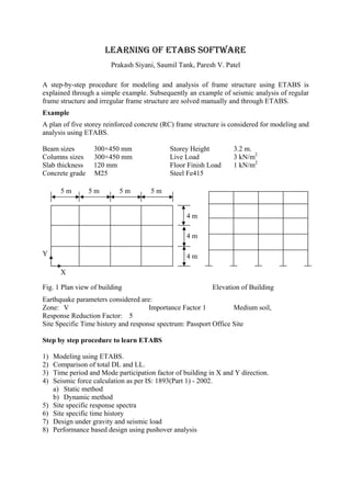
A plan of five storey reinforced concrete (RC) frame structure is considered for modeling and
analysis using ETABS.
Beam sizes 300×450 mm Storey Height 3.2 m.
Columns sizes 300×450 mm Live Load 3 kN/m2
Slab thickness 120 mm Floor Finish Load 1 kN/m2
Concrete grade M25 Steel Fe415
Fig. 1 Plan view of building Elevation of Building
Earthquake parameters considered are:
Zone: V Importance Factor 1 Medium soil,
Response Reduction Factor: 5
Site Specific Time history and response spectrum: Passport Office Site
Step by step procedure to learn ETABS
1) Modeling using ETABS.
2) Comparison of total DL and LL.
3) Time period and Mode participation factor of building in X and Y direction.
4) Seismic force calculation as per IS: 1893(Part 1) - 2002.
a) Static method
b) Dynamic method
5) Site specific response spectra
6) Site specific time history
7) Design under gravity and seismic load
8) Performance based design using pushover analysis
4 m
4 m
5 m 5 m
X
Y
5 m 5 m
4 m

ETERDCS-Nirma Uni. 25-29 May 2009
ETABS-2
Step 1: Modeling using ETABS
1) Open the ETABS Program
2) Check the units of the model in the drop-down box in the lower right-hand corner of the
ETABS window, click the drop-down box to set units to kN-m
3) Click the File menu > New model command
Note: we select No because this first model you will built
4) The next form of Building Plan Grid System and Story Data Definition will be
displayed after you select NO button.
Set the grid line and spacing between two grid lines. Set the story height data using Edit
Story Data command

ETABS-3
5) Define the design code using Options > Preferences > Concrete Frame Design
command

ETABS-4
This will Display the Concrete Frame Design Preference form as shown in the figure.
6) Click the Define menu > Material Properties
Add New Material or Modify/Show Material used to define material properties

ETABS-5
7) Define section columns and beams using Define > Frame section
Define beam sizes and click Reinforcement command to provided concrete cover
Define column sizes and click Reinforcement command to provided concrete cover and
used two options Reinforcement checked or designed

ETABS-6
8) Define wall/slab/deck
To define a slab as membrane element and one way slab define using special one way load
distribution
9) Generate the model
Draw beam using Create Line Command and draw column using Create Column
command

ETABS-7
Slab is created using 3 options in which 1st
draw any shape area, 2nd
draw rectangular area
and 3rd
create area in between grid line
Above creating option used to generate the model as shown in below figure
10) Define various loads (Dead load, live load, Earthquake load)

ETABS-8
Dead Load: self weight multiplier is used 1 to calculate dead load as default.
Live load or any other define load
1st
select the member where assign this load than click the assign button.
Assign point load and uniform distributed load
Select assigning point or member element than click the assign button

ETABS-9
11) Assign support condition
Drop-down box in the lower right-hand corner of the ETABS window,
Select only bottom single storey level to assign fixed support using
assign > Joint/Point>Restrain (Support) command
12) In building, slab is considered as a single rigid member during earthquake analysis. For
that, all slabs are selected first and apply diaphragm action for rigid or semi rigid
condition.
13) Mass source is defined from Define > mass source command. As per IS: 1893-2002,
25% live load (of 3 kN/m2
) is considered on
all floor of building except at roof level.

ETABS-10
14) Run analysis from Analysis > Run Analysis command
Step 2: Comparison of total DL and LL
Dead Load
Weight of slab = 5×12×20×0.12×24 = 345 kN
Weight of beam = 5×0.3×0.45×(12×5+20×4) ×24 = 2268 kN
Weight of column = 5×0.3×0.45×(3.2-.45) ×24 = 891 kN
Total weight = 6615 kN
Live Load
Live load = 4×12×20×3+1×12×20×1.5 = 3240 kN
Floor Finish Load
FF = 5×12×20×1 = 1200 kN
In ETABS, dead load and other loads are shown from table as shown in figure.

ETABS-11
Step 3: Time period and Mode participation factor of building in X and Y
direction.
• Static time period base on the IS 1893 is 0.075H0.75
= 0.6 sec
• Dynamic time period as per ETABS analysis is 0.885 sec in X direction and 0.698 sec in
Y direction
Time period is shown in ETABS from Display > Show Mode Shape
Mass participation factor is shown from Display > Show Table > Model Information >
Building Model Information > Model Participating Ratio.

ETABS-12
Bending moment and shear force diagram is shown from Display > Show Member Forces >
Frame/Pier/Spandrel Forces command
Bending Moment Diagram for Dead Load Shear Force Diagram for Dead Load
Select any beam or column member and press right click to shown below figure

ETABS-13
Step 4: Seismic force calculation as per IS: 1893(Part 1) - 2002.
(a) Static Method
Define static load from Define > Static load command
Press modify lateral load to shown below figure and assign various value as per IS 1893.

ETABS-14
(b) Dynamic Analysis Method
The design response spectra of IS 1893-2002 given as input in the Define menu > Response
Spectrum Functions. Response spectra load cases are define in Response Spectrum cases
The damping value is specified which is used to generate the response spectrum curve. 5%
damping factor and 9.81 (g) scale factor is assigned as shown in Figure

ETABS-15
Step 5: Site Specific Response Spectra
Site specific response spectrum is define from Define > Response Spectrum Function >
Spectrum from File.
The damping value is specified which is
used to generate the response spectrum
curve. 5% damping factor and 9.81 (g)
scale factor is assigned as shown in
Figure

ETABS-16
Step 6: Site Specific Time History
Site specific time history is define from Define > Time History Function

ETABS-17
Run the analysis and various curves is shown from Display > Show Story Response Plot

ETABS-18
Step 7: Design under Gravity and Seismic Load
Design is carried out using different combination. ETABS have facility to generate
combination as per IS 456-2000.
Select assigning combination for Design from Design > Concrete Frame Design > Select
Design Combination

ETABS-19
Design is carried out from Design > Concrete Frame Design > Start Concrete Design
Various results in form of percentage of steel, area of steel in column beam is shown from
Design > Concrete Frame Design > Display Design Information

ETABS-20
Select any beam member and left click to shown below figure

ETABS-21
Flexure detailing of beam element is shown in Figure
Shear detailing of beam element is shown in Figure

ETABS-22
Pu-Mu interaction curve, Flexural detailing, shear detailing and beam/column detailing is
shown in figure.

ETABS-23

ETABS-24
Step 8: Performance based design using pushover analysis
Design is carried out as per IS 456-2000 than select all beam to assign hinge properties from
Assign > Frame/Line > Frame Nonlinear Hinges command
Moment and shear (M & V) hinges are considered for beam element and axial with biaxial
moment (P-M-M) hinges are considered for column element as shown in Figure

ETABS-25
Defining static nonlinear load cases from Define > Static Nonlinear/Pushover command.
For push over analysis first apply the gravity loading as PUSHDOWN shown in Figure and
subsequently use lateral displacement or lateral force as PUSH 2 in sequence to derive
capacity curve and demand curve as shown in Figure. Start from previous pushover case as
PUSHDOWN for gravity loads is considered for lateral loading as PUSH 2.
Pushdown a gravity load cases
Push2 lateral load cases

ETABS-26
Run the Pushover analysis from Analysis > Run Static Nonlinear Analysis command.
Review the pushover analysis results from Display > Show Static Pushover Curve
command.

ETABS-27
Capacity spectrum, demand spectrum and performance point are shown in Figure
Show the deform shape from Display > Show Deform shape
At various stages hinge formation is shown with change the
value in step box. Step 4 is shown in this Figure.

ETABS-28

ETABS-29

ETABS-30
Illustrative Example
For the illustration purpose the data is taken from SP 22 for analysis of a 15 storey RC
building as shown in fig. 1(a). The live load on all the floors is 200 kg/m2
and soil below the
building is hard. The site lies in zone V. All the beams are of size 40 × 50 cm and slabs are 15
cm thick. The sizes of columns are 60 × 60 cm in all the storeys and wall alround is 12 cm
thick.
Analysis of the building
(a) Calculation of dead load, live load and storey stiffness: Dead loads and live loads at each
floor are computed and lumped. Stiffness in a storey is lumped assuming all the columns
to be acting in parallel with each column contributing stiffness corresponding to Kc =
12EI/L3
, where I is the moment of inertia about bending axis, L is the column height, and
E the elastic modulus of the column material. The total stiffness of storey is thus ΣKc.
The lumped mass at all floor level is 52.43 (t-s2
/m) and at roof level is 40 (t-s2
/m). The
values of I, Kc and ΣKc for all the floors / storeys are 1.08 × 108
cm4
, 9024 t/m and
180480 t/m, respectively. The value of modulus of elasticity of column material
considered is 1880000 t/m2
.
(b) For undamped free vibration analysis the building is modeled as spring mass model. As
the building is regular one degree of freedom can be considered at each floor level. Total
degrees of freedom are 15. So mass and stiffness matrix are having size 15 × 15 given as
in Table 1.
Table 1: Stiffness and mass matrix
Stiffness matrix [k] Mass matrix [m]
360960 -180480 0 0 0 0 0 0 0 0 0 0 0 0 0
-180480 360960 -180480 0 0 0 0 0 0 0 0 0 0 0 0
0 -180480 360960 -180480 0 0 0 0 0 0 0 0 0 0 0
0 0 -180480 360960 -180480 0 0 0 0 0 0 0 0 0 0
0 0 0 -180480 360960 -180480 0 0 0 0 0 0 0 0 0
0 0 0 0 -180480 360960 -180480 0 0 0 0 0 0 0 0
0 0 0 0 0 -180480 360960 -180480 0 0 0 0 0 0 0
0 0 0 0 0 0 -180480 360960 -180480 0 0 0 0 0 0
0 0 0 0 0 0 0 -180480 360960 -180480 0 0 0 0 0
0 0 0 0 0 0 0 0 -180480 360960 -180480 0 0 0 0
0 0 0 0 0 0 0 0 0 -180480 360960 -180480 0 0 0
0 0 0 0 0 0 0 0 0 0 -180480 360960 -180480 0 0
0 0 0 0 0 0 0 0 0 0 0 -180480 360960 -180480 0
0 0 0 0 0 0 0 0 0 0 0 0 -180480 360960 -180480
0 0 0 0 0 0 0 0 0 0 0 0 0 -180480 180480
52.43 0 0 0 0 0 0 0 0 0 0 0 0 0 0
0 52.43 0 0 0 0 0 0 0 0 0 0 0 0 0
0 0 52.43 0 0 0 0 0 0 0 0 0 0 0 0
0 0 0 52.43 0 0 0 0 0 0 0 0 0 0 0
0 0 0 0 52.43 0 0 0 0 0 0 0 0 0 0
0 0 0 0 0 52.43 0 0 0 0 0 0 0 0 0
0 0 0 0 0 0 52.43 0 0 0 0 0 0 0 0
0 0 0 0 0 0 0 52.43 0 0 0 0 0 0 0
0 0 0 0 0 0 0 0 52.43 0 0 0 0 0 0
0 0 0 0 0 0 0 0 0 52.43 0 0 0 0 0
0 0 0 0 0 0 0 0 0 0 52.43 0 0 0 0
0 0 0 0 0 0 0 0 0 0 0 52.43 0 0 0
0 0 0 0 0 0 0 0 0 0 0 0 52.43 0 0
0 0 0 0 0 0 0 0 0 0 0 0 0 52.43 0
0 0 0 0 0 0 0 0 0 0 0 0 0 0 40.00

ETABS-31
The first three natural frequencies and the corresponding mode shape are determined
using solution procedure of Eigen value problem i.e. Det([k] – ω2
[m]) = {0}. Time periods
and mode shape factors are given in table 2.
(c) The next step is to obtain seismic forces at each floor level in each individual mode as per
IS 1893. These calculations are shown in Table 3.
Table 2. Periods and modes shape coefficients at various levels for first three modes
Mode No. 1 2 3
Period in seconds 1.042 0.348 0.210
Mode shape coefficient at various floor levels
φ1
(r)
0.037 0.108 0.175
φ2
(r)
0.073 0.206 0.305
φ3
(r)
0.108 0.285 0.356
φ4
(r)
0.143 0.336 0.315
φ5
(r)
0.175 0.356 0.192
φ6
(r)
0.206 0.342 0.019
φ7
(r)
0.235 0.296 -0.158
φ8
(r)
0.261 0.222 -0.296
φ9
(r)
0.285 0.127 -0.355
φ10
(r)
0.305 0.019 -0.324
φ11
(r)
0.323 -0.089 -0.208
φ12
(r)
0.336 -0.190 -0.039
φ13
(r)
0.347 -0.273 0.140
φ14
(r)
0.353 -0.330 0.283
φ15
(r)
0.356 -0.355 0.353
As per clause 7.8.4.4 of IS 1893, if the building does not have closely spaced modes, the peak
response quantity due to all modes considered shall be obtained as per SRSS method. In this
example as shown below, the frequencies in each mode differ by more than 10%, so building
is not having closely spaced modes and so, SRSS method can be used.
Mode Time period Natural frequency 2π / T
1 1.042 6.03
2 0.348 18.06
3 0.210 29.92
The comparison of storey shear using SRSS method and CQC method is shown in table 3.
As per clause 7.8.2 of IS 1893 the design base shear (VB) shall be compared with base shear
(VB) calculated using a fundamental period Ta . When VB is less than VB, all the response
quantities (e.g. member forces, displacements, storey forces, storey shear and base reactions )
shall be multiplied by VB/VB.

ETABS-32
For this example
Ta = 0.075 h 0.75
for RC frame building
Ta = 0.075 (45)0.75
= 1.3031 sec
For hard soil Sa/g = 1.00/Ta = 1/1.3031 = 0.7674
VB = Ah W
W = 514.34 × 14 + 392.4 = 7593.16 t
Ah = (Z I Sa) / (2 R g)
Z = 0.36 (for zone V)
I = 1.0
R = 5.0 (considering SMRF)
Ah = (0.36 × 1 × 0.7674) / (2 × 5.0) = 0.0276
Base shear VB = 0.0276 × 7593.16 = 209.77 t
Base shear from dynamic analysis VB = 229.9 t
So, VB > VB, response quantities need not required to be modified.
The storey shear distribution along the height is shown in fig. 1 (c).
Table 3: Calculation of Seismic forces
Floor
No.
Weight
Wi (t)
Mode coefficients Wiφik Wiφik
2
φi1 φi2 φi3 Wiφi1 Wiφi2 Wiφi3 Wiφi1
2
Wiφi2
2
Wiφi3
2
1 514.34 0.037 0.108 0.175 19.030 55.548 90.009 0.704 5.999 15.751
2 514.34 0.073 0.206 0.305 37.546 105.953 156.873 2.740 21.826 47.846
3 514.34 0.108 0.285 0.356 55.548 146.586 183.104 5.999 41.777 65.185
4 514.34 0.143 0.336 0.315 73.550 172.817 162.016 10.517 58.066 51.035
5 514.34 0.175 0.356 0.192 90.009 183.104 98.752 15.751 65.185 18.960
6 514.34 0.206 0.342 0.019 105.953 175.903 9.772 21.826 60.159 0.185
7 514.34 0.235 0.296 -0.158 120.869 152.244 -81.265 28.404 45.064 12.839
8 514.34 0.261 0.222 -0.296 134.242 114.183 -152.244 35.037 25.348 45.064
9 514.34 0.285 0.127 -0.355 146.586 65.320 -182.590 41.777 8.295 64.819
10 514.34 0.305 0.019 -0.324 156.873 9.772 -166.645 47.846 0.185 53.993
11 514.34 0.323 -0.089 -0.208 166.131 -45.776 -106.982 53.660 4.074 22.252
12 514.34 0.336 -0.190 -0.039 172.817 -97.724 -20.059 58.066 18.567 0.782
13 514.34 0.347 -0.273 0.140 178.475 -140.414 72.007 61.930 38.333 10.081
14 514.34 0.353 -0.330 0.283 181.561 -169.731 145.557 64.091 56.011 41.192
15 392.40 0.356 -0.355 0.353 139.694 -139.301 138.517 49.731 49.452 48.896
Total 1778.890 588.486 346.824 498.085 498.346 498.886

ETABS-33
Table 3: Calculation of Seismic forces (Continued)
Mode 1 Mode 2 Mode 3
Mode participation factor Pk = Σ Wiφik / Σ Wi(ik2 3.571456 1.180878 0.695197
Modal mass Mk = (( Wi(ik)2/ ( Wi(ik2 6353.23 694.91 241.37
% of total mass = Mk / ( Mk 83.67 % 9.15 % 3.18 %
Time Period (Tk) 1.042 Sec 0.348 Sec 0.210 Sec
Sa/g 0.9596 2.5 2.5
Z = 0.36 (zone V), I = 1.0,
R = 5.0, Hard soil
Design horizontal spectrum value Ak = (Z I Sa) / (2 R g) 0.0345456 0.09 0.09
Base Reaction 219.44 62.54 21.72
Table 3: Calculation of Seismic forces (Continued)
Floor
No.
Qik = Akφik PkWi Vik = Σ Qik Combination of storey shear
Qi1 Qi2 Qi3 Vi1 Vi2 Vi3 SAV SRSS CQC
1 2.348 5.903 5.631 219.497 62.543 21.699 303.741 229.263 229.911
2 4.6328 11.260 9.815 217.149 56.640 16.068 289.857 224.989 225.523
3 6.854 15.579 11.456 212.516 45.379 6.253 264.148 217.397 217.745
4 9.075 18.366 10.137 205.662 29.800 -5.203 240.665 207.875 208.027
5 11.106 19.460 6.178 196.586 11.433 -15.340 223.360 197.515 197.521
6 13.073 18.694 0.611 185.480 -8.026 -21.519 215.026 186.897 186.828
7 14.914 16.180 -5.084 172.406 -26.721 -22.130 221.258 175.863 175.763
8 16.564 12.135 -9.525 157.492 -42.901 -17.045 217.440 164.119 163.973
9 18.087 6.942 -11.424 140.928 -55.037 -7.520 203.486 151.481 151.230
10 19.356 1.038 -10.426 122.841 -61.979 3.903 188.724 137.646 137.233
11 20.498 -4.865 -6.693 103.484 -63.017 14.330 180.833 122.007 121.423
12 21.323 -10.386 -1.255 82.985 -58.152 21.024 162.162 103.491 102.803
13 22.022 -14.923 4.505 61.661 -47.766 22.279 131.707 81.118 80.450
14 22.402 -18.038 9.107 39.639 -32.843 17.773 90.257 54.460 53.949
15 17.236 -14.804 8.666 17.236 -14.804 8.666 40.708 24.318 24.075

ETABS-34
4 bays @ 7.5 m = 30 m
3
bays
@
7.5
m
=
22.5m
15
storey
@
3
m
=
45
m
Fig. 1
(a) Plan and Elevation of
Building
(b) Spring and mass
model of Building
m15
m13
m14
m12
m11
m10
m9
m8
m7
m6
m5
m4
m3
m1
m2
k15
k13
k14
k12
k11
k10
k9
k8
k7
k6
k5
k4
k3
k1
k2
(c) Storey shear
distribution along
229.911 t
175.763 t
186.828 t
197.521 t
208.027 t
217.745 t
225.523 t
24.075 t
53.949 t
80.450 t
102.803 t
121.423 t
137.233 t
151.230 t
163.973 t

ETABS-35
Above mention 15 storey example solved in ETABS is describe follow:
(1) Generate model: Material properties are assign as per Indian Code. Beam, column and slab
are define as per given above dimension. 3D model of 15 story building is shown in Fig. 2.
Fig. 2 3D model of 15 storey building
(2) Static analysis load case: Loading parameters are defined as per Indian Code as shown in Fig.
3 and 4. Consider dead load and live load as a gravity load in vertical downward direction
and earthquake load as lateral load in horizontal direction. Earthquake load is defined as per
IS 1893-2002.
Fig. 3 Define static load case

ETABS-36
Fig. 4 Define a seismic loading as per IS: 1893-2002
(3) Dynamic analysis: IS 1893 response spectrum curve for zone V is shown in Fig. 5. The
damping value of 5% is specified to generate the response spectrum curve. The scale factor
of 9.81 (i.e. g) is assigned as shown in Fig. 6.
Fig. 5 IS 1893 response Spectra Graphs Fig. 6 Response Spectra Case Data
(4) The design acceleration time history for passport office site is given as input in Define menu
> Time History Function. The time history load cases are defined from the Time History
Cases option as shown in the Fig. 7. The acceleration time history of Passport office site as
defined in ETABS is shown in Fig. 8.

ETABS-37
Fig. 7 Time History Options
Fig. 8 Time History Graphs
Time history case data is defined for simplicity of analysis. Number of output time steps is
300. Linear analysis case and two direction acceleration load case are considered. The scale
factor 9.81 i.e. gravitational acceleration (m/sec2
) and 5% damping are defined as shown in
Fig. 9.
Fig. 9 Time History Case Data
(5) Mass source is defined in modeling as shown in Fig. 10. As per IS: 1893-2002, 25% live load
(of 200 kg/m2
) is considered on all floor of building except at roof level.

ETABS-38
(6) In building, slab is considered as a single rigid member during earthquake analysis. ETABS
has a facility to create rigid diaphragm action for slab. For that, all slabs are selected first and
apply diaphragm action for rigid or semi rigid condition.
Fig. 10 define mass source Fig. 11 Rigid diaphragm in plan
Results of Static and Dynamic analysis
Fig. 12 Time Period of different mode
Table 4 percentage of total seismic mass
Table 5 Base reaction for all modes
1.1097 sec 0.2243 sec
0.3712 sec

ETABS-39
Compare manual static and dynamic results with ETABS static and dynamic results
Table 6. Periods and modes shape coefficients at various levels for first three modes
Table 7. Compare the time period, mass participation and base reaction
Manual analysis ETABS Analysis
Mode No. 1 2 3 1 2 3
Period in seconds 1.042 0.348 0.210 1.109 0.371 0.224
Mode shape coefficient at various floor levels
φ1
(r)
0.037 0.108 0.175 0.036 0.109 0.175
φ2
(r)
0.073 0.206 0.305 0.073 0.206 0.304
φ3
(r)
0.108 0.285 0.356 0.109 0.283 0.356
φ4
(r)
0.143 0.336 0.315 0.143 0.336 0.315
φ5
(r)
0.175 0.356 0.192 0.175 0.356 0.195
φ6
(r)
0.206 0.342 0.019 0.206 0.342 0.023
φ7
(r)
0.235 0.296 -0.158 0.234 0.297 -0.154
φ8
(r)
0.261 0.222 -0.296 0.261 0.224 -0.290
φ9
(r)
0.285 0.127 -0.355 0.283 0.129 -0.354
φ10
(r)
0.305 0.019 -0.324 0.304 0.023 -0.327
φ11
(r)
0.323 -0.089 -0.208 0.322 -0.086 -0.213
φ12
(r)
0.336 -0.190 -0.039 0.336 -0.186 -0.045
(13 (r) 0.347 -0.273 0.140 0.345 -0.270 0.134
(14 (r) 0.353 -0.330 0.283 0.351 -0.327 0.277
(15 (r) 0.356 -0.355 0.353 0.356 -0.354 0.351
Mode
Time period (sec)
Percentage of Total
Seismic Mass
Base reaction (kN)
Manual ETABS Manual ETABS Manual ETABS
1 1.042 1.109 83.67 83.64 2194.40 2109.86
2 0.348 0.371 9.15 9.16 625.43 635.94
3 0.210 0.224 3.18 3.20 217.21 222.43

ETABS-40
Table 8 comparison of Static Dynamic and Time history analysis
Static Analysis Dynamic Analysis
Passport office Site
Time History Analysis
Story No.
Story Shear (kN) Story Force (kN) Story Shear (kN) Story Force (kN)
Story Shear
(kN)
Story Force
(kN)
Manual ETABS Manual ETABS Manual ETABS Manual ETABS ETABS ETABS
15 303.55 325.46 303.55 325.46 243.10 252.87 243.10 252.87 114.15 114.15
14 650.00 673.89 346.46 348.43 544.60 545.14 301.50 292.27 250.58 136.43
13 948.73 974.33 298.73 300.44 811.10 801.74 266.50 256.60 378.82 128.24
12 1203.27 1230.33 254.54 256.00 1034.90 1015.87 223.80 214.13 495.44 116.62
11 1417.16 1445.43 213.88 215.10 1220.00 1191.48 185.10 175.61 598.18 102.74
10 1593.92 1623.21 176.76 177.78 1376.40 1338.91 156.40 147.43 686.07 87.89
9 1737.10 1767.20 143.18 143.99 1514.80 1468.49 138.40 129.58 759.32 73.25
8 1850.23 1880.98 113.13 113.78 1641.10 1586.46 126.30 117.97 819.05 59.73
7 1936.84 1968.09 86.61 87.11 1758.60 1695.82 117.50 109.36 866.9 47.85
6 2000.48 2032.09 63.64 64.00 1868.90 1799.56 110.30 103.74 904.69 37.79
5 2044.67 2076.53 44.19 44.44 1975.10 1901.64 106.20 102.08 934.11 29.42
4 2072.95 2104.97 28.28 28.44 2078.70 2003.54 103.60 101.90 956.48 22.37
3 2088.86 2120.97 15.91 16.00 2173.90 2099.83 95.20 96.29 972.71 16.23
2 2095.93 2128.09 7.07 7.12 2249.80 2177.58 75.90 77.75 983.34 10.63
1 2097.70 2129.86 1.77 1.77 2292.60 2221.55 42.80 43.97 993.82 10.48
0 2097.70 2130.00 0.00 0.00 2292.60 2221.60 0.00 0.00 993.82 0

ETABS-41

ETABS-42
TORSION ANALYSIS OF BUILDING
EXAMPLE: A four storeyed building (with load 300 kg/m2
) has plan as shown in Fig. 1 and
is to be designed in seismic zone III. Work out the seismic shears in the various storeys of the
proposed building. The foundation is on hard soil and importance factor is 1.0 (Data from
SP- 22 : 1982)
As building is having height 12 m and is in zone III, earthquake forces can be calculated by
seismic coefficient method using design spectrum.
(a) Lumped mass Calculation
Total weight of beams in a storey = 27 × 7.5 × 0.4 × 0.5 × 2.4 = 97.2 t
Total weight of columns in a storey = 18 × 3 × 0.4 × 0.6 × 2.4 = 31.10 t
Total weight of slab in a storey = (22.5 × 15 + 15 × 15) × 0.15 × 2.4 = 202.5 t
Total weight of walls = (22.5 + 15 + 7.5 +30 + 15 + 15 – 6 × 0.6 – 8 × 0.4) × 0.2 × 3 × 2.0
= 117.8 t
Live load in each floor = (22.5 × 15 + 15 × 15 ) × 0.3 × 0.25 = 42.18 t
Lumped weight at floor 1, 2 and 3 = Dead load + Live load
= ( 97.2 + 31.10 + 202.5 + 117.8) + 42.18 = 490.8 t
Lumped weight at roof floor = Dead load
( 97.2 + 31.10/2+ 202.5 + 117.8/2 ) = 374.17 t
Total weight of building W = 490.8 × 3 + 374.17= 1846.57 t
(b) Base shear calculation:
Base shear VB = Ah W
Ah = (Z I Sa) / (2 R g)
Z = 0.16 (Zone III)
I = 1.0
R = 5 (considering SMRF)
T = 0.075 × h0.75
= 0.075 × 120.75
= 0.4836 sec
Sa/g = 1/0.4836 = 2.07
Ah = (0.16 × 1.0 × 2.07) / (2 × 5) = 0.033
VB = 0.033 × 1846.57 = 60.94 t
(c) Shear force in various storeys
Calculation of storey shear distribution along height is shown in Table 1.

ETABS-43
(d) Calculation of eccentricity
Assuming mass is uniformly distributed over the area
Horizontal distance of center of mass
Xm = (15 × 22.5 × 7.5 + 15 × 15 × 22.5) / (15 × 22.5 + 15 × 15) = 13.5 m
Vertical distance of center of mass
Ym = (15 × 22.5 × 11.25 + 15 × 15 × 7.5) / (15 × 22.5 + 15 × 15) = 9.75 m
As columns are of equal size their stiffness are also same. So horizontal distance of center of
rigidity,
Xr = (4 × 7.5 + 4 × 15 + 3 × 22.5 + 3 × 30) / 18 = 13.75 m
Vertical distance of center of rigidity,
Yr = (5 × 7.5 + 5 × 15 + 3 × 22.5) / 18 = 10 m
Static eccentricity in X direction = esi = Xr – Xm = 13.75 – 13.5 = 0.25m
Design eccentricity in X direction = 1.5 × 0.25 + 0.05 × 30 = 1.875 m
Or = 0.25 – 1.5 = -1.25 m
Static eccentricity in Y direction = esi = Yr – Ym = 10.00 – 9.75 = 0.25m
Design eccentricity in Y direction = 1.5 × 0.25 + 0.05 × 22.5 = 1.5 m
Or = 0.25 – 1.125 = -0.875 m
The center of mass and center of rigidity and design eccentricity are shown in Fig. 2.
Total rotational stiffness Ip = Σ(Kx y2
+ Ky x2
)
Kx = Stiffness of one column in X direction = 12 EI / L3
= 12 × 1880000 × (0.6 × 0.43
/12)/33
= 2673.78 t/m
Ky = Stiffness of one column in Y direction = 12 EI / L3
= 12 × 1880000 × (0.4 × 0.63
/12)/33
= 6016.00 t/m
Kx y2
= 2673.78 × (5(102
) + 5(2.52
) + 5(52
) + 3(12.52
)) = 3008002.5
Ky x2
= 6016.0 × (4(13.752
) + 4(6.252
) + 4(1.252
) + 3(8.752
) + 3(16.252
))
= 11674799.0
Ip = 3008002.5 + 11674799.0 = 14682802.5
(e) Torsional due to seismic force in X direction
Torsional moment T at various floors is considering seismic force in X direction only is
shown in Table 3.
Torsional shear at each column line is worked out as follows using following equation:

ETABS-44
Vx = (T/Ip) × y × Kxx
Kxx = 5 × Kx (for column line 1, 2, 3 )
= 3 × Kx (for column line 4 )
Kyy = 4 × Ky (for column line A, B, C )
= 3 × Ky (for column line D, E )
Additional shear due to torsional moments in columns at various floor levels are shown in
Table 4.
(f) Torsional due to seismic force in Y direction
Torsional moment T at various floors is considering seismic force in Y direction only is
shown in Table 5.
Torsional shear at each column line is worked out as follows using following equation:
Vy = (T/Ip) × x × Kyy
Additional shear due to torsional moments in columns at various floor levels are shown in
Table 6.
As per the codal provisions only positive values or additive shear should be considered. This
shear is to be added in to shear force resisted by columns due to seismic force in respective
directions.
X
Y
D
C
B
A E
4
3
2
1
4 @ 7.5 m = 30 m
3
@
7.5
m
=
22.5m
Fig. 1 Example

ETABS-45
Table:1 Storey shear at various floors (manual)
Floor Wi t hi m Wihi
2
Qi t Vi t
1 490.8 3 4417.20 2.32 60.94
2 490.8 6 17668.80 9.30 58.61
3 490.8 9 39754.80 20.93 49.30
4 374.17 12 53880.48 28.37 28.37
1157212.80
Cm
Cr
Fig. 2 Position of Center of Mass, Center of Rigidity and Design Eccentricities
EQY
Xm = 13.5 m
Xr = 13.75 m
Ym
=
9.75
m
Yr
=
10.0
m
EQX
EQX
EQY
0.875 m
1.50 m
1.25 m
1.875 m
Fig. 3 Plan and 3D view of modeled building in ETABS

ETABS-46
Table: 2 Storey shear (tone) from ETABS
Floor Weight
of each
storey
height Storey
shear
1 487.55 3.00 59.90
2 487.55 6.00 57.66
3 487.55 9.00 48.70
4 388.13 12.00 28.54
18507.74 - 13632.27 =4875.5 kN (seismic
weight of first storey)
Fig. 4 Storey shear (kN) in ETABS for earthquake in X direction
Fig. 5 Centre of mass and centre of rigidity at each storey in ETABS

ETABS-47
Table: 3 Torsional moment due to seismic force in X direction
Torsional moment in edi = 1.5 m edi = -0.875 m
Storey 1 T1 60.94× 1.5 = 91.41 -53.32
Storey 2 T2 58.61× 1.5 = 87.92 -51.28
Storey 3 T3 49.30× 1.5 = 73.96 -43.14
Storey 4 T4 28.37× 1.5 = 42.56 -24.82
Table: 4 Additional shear due to seismic force in X direction
Column
line
First storey
(shear in one column)
Total
shear
from
ETABS
Second storey
Total
shear
from
ETABS
Third storey
Total
shear
from
ETABS
Fourth Storey
Total
shear
from
ETABS
Direct
Torsional
Shear Vx
Total Direct
Torsional
Shear Vx
Total Direct
Torsional
Shear Vx
Total Direct
Torsional
Shear Vx
Total
1 y = 10
m
3.39 + 0.83 4.22 16.79
3.26
0.80 4.06 16.30
2.74
+0.67 3.41 13.63 1.58 +0.39 1.97 7.86
(-0.49) 2.90 (-0.47) 2.79 (-0.39) 2.35 (-0.23) 1.35
2 y = 2.5
m
3.39 +0.21 3.60 16.80
3.26
0.20 3.46 16.45
2.74
+0.17 2.91 13.70 1.58 +0.10 1.68 7.92
(-0.12) 3.27 (-0.12) 3.14 (-0.10) 2.64 (-0.06) 1.52
3 y = 5 m
3.39 -0.42 2.97 16.80
3.26
-0.40 2.86 16.55
2.74
-0.34 2.40 13.75 1.58 -0.19 1.39 7.96
(+0.24) 3.63 (+0.23) 3.49 (+0.20) 2.94 (+0.11) 1.69
4 y =
12.5 m
3.39
-0.62 2.77 9.48
3.26
-0.60 2.66 8.28
2.74
-0.51 2.23 7.36
1.58
-0.29 1.29 4.10
(+0.36) 3.75 (+0.35) 3.61 (+0.29) 3.03 (+0.17) 1.75
62.18
59.87
59.81
57.58
50.28
48.43
29.00
27.85
60.17 57.86 48.73 27.98

ETABS-48
Fig. 6 Shear force (kN) in column line 1 and line 2 due to earthquake force in X direction
Fig. 7 Shear force (kN) in column line 3 and line 4 due to earthquake force in X direction

ETABS-49
Table: 5 Torsional moment due to seismic force in Y direction
Table: 6 Additional shears due to seismic force in Y direction
Torsional moment in edi = 1.875 m edi = -1.25 m
Storey 1 T1 60.94 × 1.875 = 114.26 -76.18
Storey 2 T2 58.61 × 1.875 = 109.90 -73.27
Storey 3 T3 49.30 × 1.875 = 92.45 -61.64
Storey 4 T4 28.37 × 1.875 = 53.20 -35.47
Column
line
First storey
Total
shear
from
ETABS
Second storey
Total
shear
from
ETABS
Third storey
Total
shear
from
ETABS
Fourth Storey
Total
shear
from
ETABS
Direct
Torsional
Shear Vy
Total Direct
Torsional
Shear Vy
Total Direct
Torsional
Shear Vy
Total Direct
Torsional
Shear Vy
Total
A x =
13.75 m
3.39
+2.57 5.96 13.44
3.26
+2.48 5.74 12.88
2.74
+2.08 4.82 10.87
1.58
+1.20 2.78 6.25
(-1.72) 1.67 (-1.65) 1.61 (-1.39) 1.35 (-0.80) 0.78
B x =
6.25 m
3.39
+1.17 4.56 13.485
3.26
+1.13 4.39 13.16
2.74
+0.95 3.69 11.00
1.58
+0.54 2.12 6.38
(-0.78) 2.61 (-0.75) 2.51 (-0.63) 2.11 (-0.36) 1.22
C x =
1.25 m
3.39 -0.23 3.16 13.514
3.26
-0.22 3.04 13.40
2.74
-0.19 2.55 11.11 1.58 -0.11 1.47 6.50
(+0.16) 3.55 (+0.15) 3.41 (+0.13) 2.87 (+0.07) 1.65
D x =
8.75 m
3.39
-1.23 2.16 9.707
3.26
-1.18 2.08 8.99
2.74
-0.99 1.75 7.69
1.58
-0.57 1.01 4.33
(+0.82) 4.21 (+0.79) 4.05 (+0.66) 3.40 (+0.38) 1.96
E x =
16.25 m
3.39
-2.28 1.11 9.721
3.26
-2.20 1.06 9.15
2.74
-1.85 0.89 7.77
1.58
-1.06 0.52 4.40
(+1.52) 4.91 (+1.46) 4.72 (+1.23) 3.97 (+0.71) 2.29
64.48
59.87
62.03
57.58
52.15
48.43
30.00
27.85
58.63 56.36 47.42 27.28

ETABS-50
Fig. 8 Shear force (kN) in column line A, B and C due to earthquake force in Y direction
Fig. 9 Shear force (kN) in column line D and E due to earthquake force in Y direction

47918582.pdf

Recommended

Recommended

More Related Content

Similar to 47918582.pdf

Similar to 47918582.pdf (20)

Recently uploaded

Recently uploaded (20)

47918582.pdf