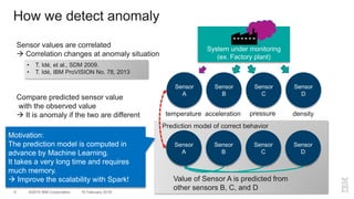
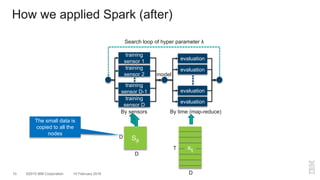
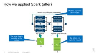
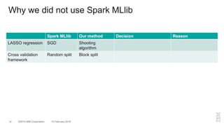
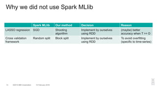
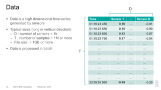
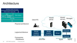
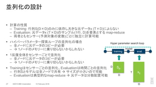
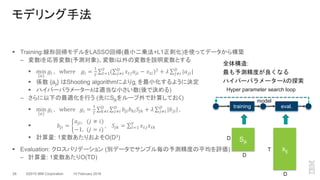
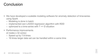
The document outlines a method for developing software for scalable anomaly detection in time-series data using Apache Spark. It discusses the implementation of a prediction model that compares observed sensor data with predicted values to identify anomalies, and details the use of lasso regression for training the model. Performance improvements and challenges faced during the process, such as order preservation in RDD operations and the use of alternative APIs, are also highlighted.


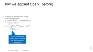
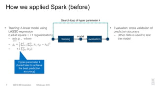
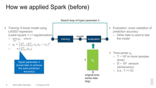
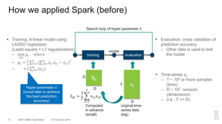


![[212]big models without big data using domain specific deep networks in data-...](https://cdn.slidesharecdn.com/ss_thumbnails/212bigmodelswithoutbigdatausingdomain-specificdeepnetworksindata-scarcesettings-171017003514-thumbnail.jpg?width=640&height=640&fit=bounds)


![7.__Developing_a_Research_Proposal[1].pptx](https://cdn.slidesharecdn.com/ss_thumbnails/7-260131073037-df92dd7d-thumbnail.jpg?width=640&height=640&fit=bounds)


