Yet Another Performance Profiling Method Oracle: end of tuning by ratios

1. Yet Another Performance Profiling Method
(Or YAPP-Method)
Anjo Kolk, Shari Yamaguchi – Data Server Applied Technologies
Jim Viscusi -- Oracle Support Services Centers of Expertise
Oracle Corporation
June 1999
Technical Paper

2. YAPP Method
June 1999 2
TABLE OF CONTENTS
I. INTRODUCTION.............................................................................................................................3
II. DEFINITIONS.................................................................................................................................3
THE 80/20 RULE ..................................................................................................................................3
RESPONSE TIME ...................................................................................................................................3
SCALABILITY .......................................................................................................................................3
VARIABLES THAT AFFECT SCALABILITY - HOW TO MONITOR AND MEASURE ........................................5
III. TUNING RESPONSE TIME ........................................................................................................6
DETERMINE FOR WHICH LEVEL RESPONSE TIME IS BEING MEASURED...................................................7
SET INIT.ORA PARAMETER TIMED_STATISTICS = TRUE..............................................................7
CALCULATE THE TOTAL RESPONSE TIME ..............................................................................................7
IV. BREAKING DOWN CPU TIME..................................................................................................9
V. BREAKING DOWN WAIT TIME...............................................................................................11
VI. PARALLEL SERVER EVENTS AND TUNING ......................................................................20
VII. ADDITIONAL DISCUSSIONS AND EXAMPLES.................................................................24
VIII. CONCLUSION..........................................................................................................................26
IX. ACKNOWLEDGEMENTS .........................................................................................................26

3. YAPP Method
June 1999 3
I. Introduction
Traditional Oracle database performance tuning methodologies based on ratios are quickly
becoming outdated and unusable as applications and databases continue to grow significantly
across varying types of businesses. The “Ratio Tuning” technique involves finding bad ratios
(e.g., the buffer cache hit ratio, latch-hit ratio) and addressing each separately. This technique
is very simple and straightforward, but becomes ineffective as systems become more
complex. Additionally, ratio tuning implies that the whole system consists of identical
components, but large workflow applications may contain a single bottleneck within its design.
Such a bottleneck rarely surfaces immediately when following the traditional tuning approach.
Therefore, a more holistic approach is needed to better understand and tune these large and
complex mission critical systems. This involves first reviewing all relevant data (i.e., the ratios
and other relevant information) and then planning a course of action that focuses attention on
the bigger impact issues.
This paper will discuss a simple holistic method. In addition, you will understand why tuning
the application and SQL statements will have a much greater impact on overall performance
than other components.
II. Definitions
Since the definition of common terms tend to differ depending on the context of the topic, it is
imperative that we clearly define the terms referenced in this paper. Some definitions may
appear simple, but the simplicity of this method makes it work successfully. This paper
adheres to the saying, “Common sense before hard work” (first decide what direction to run,
then start running).
The 80/20 Rule
The 80/20 rule, conceived by Vilfredo Pareto, underlies our tuning methodologies. It states
that a minority of causes, inputs, or efforts usually produces a majority of the results, outputs,
or rewards. This implies that there is a built in imbalance between causes and results, inputs
and outputs, effort and reward. Although our tuning method primarily focuses on a small
subset of the available performance statistics, the analyzed output and resultant tuning actions
will provide the largest percentage of overall performance improvement. The goal is to
simplify and exert the least amount of effort, while still achieving significant results.
Response time
In general terms, response time can be described as follows:
Response Time = Service Time + Wait Time
If service time and/or wait time is high, it will directly impact the total response time. The
Oracle database dynamic views provides statistics that allow one to calculate the total service
time and the total wait time within the database. However, the calculated response time will
always be less than or equal to the actual response time observed by the end user. The
difference is due to external forces, such as network latency or queuing latency (if TP
monitors or Web Servers are used).
Scalability
As businesses and business needs grow, customers look for scalable solutions. The need for
scalability (increased throughput) and/or speedup (faster response time) is quickly becoming a
necessity in the world of complex systems. However, the following questions are rarely
answered thoroughly:
• What is scalability?

4. YAPP Method
June 1999 4
• How is scalability and performance actually measured?
• What areas affect the ability to scale?
The answers are important since this will help to determine how well a system is currently
performing and how well it can be expected to perform in the future as an application grows.
A scalable solution is one that will allow a business application to grow in complexity and user
base while continuing to perform within expected and projected guidelines.
There are 4 basic ‘logical’ areas where scalability can be examined:
„hardware
„operating system
„database
„application
It is also important to look at the ‘physical’ areas that affect scalability:
„network
„memory
„CPU
„I/O
Most performance issues do not originate directly from the database, so the question
becomes – “Where is the problem?” We have found that more than 80% of them are rooted
within the application due to bad design or inefficient implementations. From this, it can be
seen that the highest percentage of performance improvements can be achieved by making
changes in the application.
So, given this statement, why do people usually focus on the Oracle database? Generally, it is
a victim of its capabilities. As a first effort, database administrators and users focus on the
database since it supplies easy access to a wealth of statistics about its performance. In
addition, application tuning may not be simple or straightforward. Applications are designed
around business rules and processes. Sometimes, finding algorithms that fully conform to
business rules while achieving optimal database performance is impossible or extremely
difficult. Other reasons may be cost related, such as the discovery that a poorly designed
application has already been implemented, either internally by a project team or externally
through special consultants, and necessary changes will incur greater costs.
Example 1:
Consider a business rule dictating that every row inserted into a table must contain a
unique, sequential number. If multiple transactions want to insert into the same table,
the resulting application design can only allow one active transaction at a time. To
guarantee continuousness, the next transaction must wait for the current transaction
to commit or rollback before it can safely decide to either allocate the next sequence
number or reuse the current one. The performance cost is that your transactions
must run serially even if hardware resources are available to run more processes and
the database engine is capable of managing many concurrent transactions.
.
Example 2:
A real life example may be a bank that requires the bank manager to approve each
check cashed. If there are three tellers servicing customers who are all cashing
checks but only one bank manager qualified to approve the checks, then this process
will not scale well. The bank becomes serialized around the manager. The bank may
consider hiring and training more managers, but that would increase business costs.
A more cost-effective solution would be to relax the business rule that requires each
check to be signed by the manager for approval. In this case, changing the business
rule could yield better scalability at a lower cost.

5. YAPP Method
June 1999 5
Variables that affect scalability - How to monitor and measure
What affects scalability, and how can it be monitored and measured? Basically, the ability for
an application to scale is directly affected by the synchronization of access to common
resources. For example, only one process may modify a given row at one time. Other
processes requesting to make a modification to the same row must wait for the first process to
either commit or rollback. So the ability to scale will be affected by how often the application
needs to synchronize (the amount of synchronization) and how expensive it is to synchronize
(the cost of synchronization).
Therefore:
Scalability ←
←
←
← Amount of Synchronization x Cost of Synchronization
(Note: the Amount of Synchronization may also be stated in terms of the Rate of
Synchronization. Amount and Cost can actually be qualified in absolute terms, but it would be
better to think of them in relative terms most of the time.)
Take the following example:
Given a computer system that does a certain amount of I/O at a certain cost per I/O. If
the disk drives are upgraded from 4500 RPM to 5400 RPM models, the cost of an I/O is
20 percent cheaper and the total I/O scalability will improve by 20 percent.
In this example, one interprets the Cost of Synchronization as the wait time. Waiting on a
resource that is being used by another session means another delay that can be added to the
total Cost of Synchronization. Reducing the wait time could improve the scalability of the
system. So:
Cost of Synchronization →
→
→
→ Average Wait Time
This means that if there is no wait time, the system could scale almost perfectly. It also
follows that tuning a system to reduce the wait time can help achieve a significant
performance and scalability improvement. This assumes that there is no “busy waiting”. Busy
waiting occurs when the process waiting for a resource consumes CPU when it should
otherwise place itself on a wait queue. An example of “busy waits” is a process spinning while
trying to acquire a latch.
One could interpret the Amount of Synchronization as the number of times a process waited.
For Oracle processes, this can be found in the Oracle statistics as the Total Waits
(v$system_event and v$session_event).
An example of synchronization would be a comparison between Oracle's single instance
environment and the Oracle Parallel Server (OPS) environment. Within an Oracle single
instance environment, synchronizing changes to blocks in the Oracle buffer cache can be
managed through latches since the blocks being modified reside within a single node.
However with OPS, synchronization requires expensive instance locks in order to coordinate
access to common resources shared across multiple nodes and the disjoint buffer caches.
Since locking in OPS becomes more expensive, the synchronization overhead increases. The
following table compares the costs of different synchronization methods:
Type of synchronization Cost
1
Relative Cost
Latches 0.000001sec 1 sec
Enqueues 0.0001 sec 100 sec
Instance locks 0.01 sec 10000 sec
1
The timings are fictional, it just illustrates that there is an order of magnitude difference between the synchronization costs for
the different types of synchronization.

6. YAPP Method
June 1999 6
This table implies that when an application is migrated from single-instance Oracle to Oracle
Parallel Server, the cost of synchronization will increase (the local enqueues will become
global enqueues, or instance locks). Therefore, scalability will be affected. Two things can be
done about this:
„reduce the Cost of synchronization
In this example, that will be difficult to accomplish as the cost of instance locks will be
more or less fixed. The cost of synchronization will be reduced only when upgrading
software, improving interconnects, or installing faster CPUs.
„reduce the Amount of synchronization
This is something that is tangible and can be affected by tuning or changing the
application so that the amount of enqueues requested is reduced. A common approach to
this is partitioning the application so users are not accessing the same set (partition) of
data (resource).
The Amount and Cost of synchronization will directly affect the ability for an application to
scale. Statistics from the operating system and Oracle can be used to determine what events
are contributing most to the amount and cost of synchronization. The method using these
tools will be described in the following sections.
III. Tuning Response Time
When discussing performance and tuning problems, it is important to remember that the
primary goal can be one of the following (or both):
1. Improve response times
As stated before, response time is the sum of service time and wait time. Improving
response time means reducing one or both of these components. Obviously, one begins
by choosing the component with the largest room to tune. For example, if the service time
is 20 percent of the total, improving it will not impact response time very much. If tuning
efforts cut the service time by 50 percent, then this portion of the response time will only
drop from 20 percent to around 10 percent. This implies overall response time may only
improve by at most 10 percent. However, focusing effort to improve the wait time by 50
percent translates to a 40 percent increase in response time!
2. Improve throughput
This can be a bit more complicated. If an application is running out of available CPU on
the system, there is a need to reduce the service time. A simple, but expensive solution
would be to replace the existing CPUs with faster ones or add more CPUs. However, it is
also possible to redesign each batch or user process to do more work. Another solution
would be to reduce the wait time of the process, thus improving the overall response time.
Once a process can complete each transaction quicker, it can execute more transactions
over the same span of time.
It is important to identify the desired percentage of performance improvement. For example, a
user may require a 30% response time or throughput improvement. Relying on older classes
and papers, many DBAs and Support analysts calculate certain, well-known ratios and
address those that are deemed “bad.” Trying to improve these bad ratios, without considering
how much the change will contribute to overall performance, usually will fail to provide
noticeable improvement. For example, increasing the parameter spin_count may achieve a
5% performance gain (or even decrease performance further since the system might be
already CPU-bound) whereas introducing more efficient SQL or redistributing I/O may achieve
a 40% performance gain. Although rewriting an application or purchasing hardware may be
expensive, determining the performance benefit before weighing the cost is also important.
The following method can determine what events contribute the largest synchronization cost,

7. YAPP Method
June 1999 7
which can ultimately be related to the total response time for a user. So how can the Oracle
response time be measured?
First, we must define the unit of work for which response time is being measured, and
determine if this is being monitored at the instance level or session level. Based on the unit of
work, the following views can be used to determine the total response time:
• V$SYSSTAT and V$SYSTEM_EVENT for the instance level
• V$SESSTAT and V$SESSION_EVENT for the session level
Determine for which level response time is being measured
The response time can be measured on the instance level (although this may be very rough
and not precise enough) or the session level (not easily available if sessions have a short
lifetime). The following is a closer look at the levels of response time calculations to use:
• system/instance level
Use the instance level if sessions logon/logoff frequently. This will result in a general
overview of what could be wrong with the instance.
• session level
If sessions stay connected for a long time, looking at the session level is more
beneficial. It will allow direct measurement of response times.
Set init.ora parameter TIMED_STATISTICS = true
Enabling timed_statistics is necessary to properly analyze the performance within
Oracle. On most platforms, this feature introduces a small (2-3%) overhead, but returns the
much greater benefit of enabling the determination of performance bottlenecks. Many
sources of tuning information recommend disabling timed_statistics due to perceived
overhead (which was larger on some older operating systems), but tuning a system without
that valuable information becomes an almost impossible task. Note that as of Oracle7 R7.3,
you can dynamically change the setting of timed_statistics: alter system
timed_statistics = TRUE or alter session timed_statistics = TRUE
Calculate the total response time
This section covers how to retrieve the relevant statistics from the Oracle performance tables
used to calculate total response time. To restate the original response time formula:
Response Time = Service Time + Wait Time
Service Time
The service time is equal to the statistic “CPU used by this session” which is shown through
entries in V$SYSSTAT or V$SESSTAT by selecting for this event.
Use v$statname to assist in finding the correct statistic number for “CPU used by this
session” for each platform and release. This event represents the total amount of CPU time
used. (Note: v$sysstat does not include CPU used by the Oracle background processes
and v$sesstat doesn’t show the amount of CPU used per Oracle background process).
Instance level
select a.value “Total CPU time”
from v$sysstat a
where a.name = ‘CPU used by this session’;
Session level
select sid, a.value “Total CPU time”
from v$sesstat a

8. YAPP Method
June 1999 8
where a.statistic# = 12 // statistic # for ‘CPU used by
this session’ - obtained from
v$statname
Some platforms may also provide Operating System (OS) specific statistics that better
indicate how CPU time was used. For example:
OS User time
This will show the amount of user time used out of the total CPU time.
OS System time
This will indicate the amount of system time (for system calls) used out of the total
CPU time.
Add OS User time and OS System time to get the total amount of CPU time used. Note that
this will always be more than “CPU used by this session.” The difference can be explained by
how Oracle measures the CPU used by a session. Measurement occurs at a user call level.
When the user call starts, a CPU time stamp is taken, and when the call completes, that time
stamp is subtracted from the current CPU time. The granularity is 1/100 of a second. So, if
the user call completes within 1/100 of a second, the difference will be 0. Additionally, some
of the network interactions are not measured in “CPU used by this session”. This means, for
example, that some character set conversions and/or datagram packaging are not accounted
for.
utlbstat/utlestat
This information can also be seen in a historical context using utlbstat.sql and
utlestat.sql scripts. The output of these scripts calculates the 'CPU used by this session'
as the cumulative amount of CPU that all sessions have used during the sample period – so
the name is rather misleading!
Wait Time
The wait time is recorded through entries in V$SYSTEM_EVENT or V$SESSION_EVENT, by
summing the time waited for all the events excluding those waited for due to the foreground
process and all background waits. One may ignore the following wait events:
• client message
• dispatcher timer
• KXFX: execution message dequeue – Slaves
• KXFX: Reply Message Dequeue – Query Coord
• Null event
• parallel query dequeue wait
• parallel query idle wait - Slaves
• pipe get
• PL/SQL lock timer
• pmon timer
• rdbms ipc message
• slave wait
• smon timer
• SQL*Net message from client
• virtual circuit status
• WMON goes to sleep
Instance Level
select sum(time_waited) “Total Wait Time”
from v$system_event

9. YAPP Method
June 1999 9
where event not in (‘pmon timer’, ‘smon timer’, ‘rdbms ipc
message’, ‘parallel dequeue wait’, ‘virtual circuit’, ‘SQL*Net
message from client’, ‘client message’, ‘NULL event’);
Note: not a complete list in this sample query
Session Level
select sid, sum(time_waited) “Total Time waited”
from v$session_event
where event != ‘SQL*Net message from client’
group by sid;
utlbstat/utlestat
The above information is also available from the report.txt file generated by the
utlbstat/utlestat scripts. Collect all relevant wait times (excluding the ones listed above) from
the sections on background and non-background wait events.
Tuning to change overall response time
Once all this data has been acquired, we can rationally decide where to focus our tuning
efforts, by basing our focus on the area that is taking the highest percentage of time. The
above steps simply present a method for looking initially at the entire system and then logically
determining which area contributes most to the total response time. The next step involves
breaking down this target area and taking appropriate action.
Keep in mind, that once all this data has been gathered the problem may not be at the
database level. Any tuning activity needs to take the entire system into account, and we need
to apply the same principle we use when decomposing response time on the server to the
overall system. To illustrate this, consider a query where the response time is 10 seconds.
Your investigation decomposes that into Service time and Wait time, but a quick look at the
numbers shows that the total amount of time spent in the database is only 2 seconds.
Therefore, the database server is accounting for only 20% of the overall response time and
may not be the best area to focus your tuning efforts.
IV. Breaking Down CPU Time
If CPU contributes most to total response time, it will need to be further decomposed into
detailed segments to properly understand the problem.
CPU time basically falls into three categories:
parse time CPU
This reports the amount of CPU used for parsing SQL statements. Generally, parse time
CPU should not exceed 10 to 20% of the total CPU, although many times this is around
70%. Parse time CPU can be a strong indication that an application has not been well
tuned (or an older version of Forms such as v4.0 or below is still being used). High parse
time CPU usually indicates that the application may be spending too much time opening
and closing cursors or is not using bind variables. Check the following statistics from
V$SYSSTAT or V$SESSTAT:
• parse count
This is the total number of hard and soft parses. A hard parse occurs when a
SQL statement has to be loaded into the shared pool. In this case, Oracle has to
allocate memory in the shared pool and parse the statement. A soft parse is
recorded when Oracle checks the shared pool for a SQL statement and finds a
version of the statement that it can reuse.

10. YAPP Method
June 1999 10
In Oracle7, one cannot distinguish between hard and soft parses. In Oracle8,
parse count is divided into two statistics: parse count (total) and parse count
(hard). By subtracting the parse count (hard) from parse count (total) one can
calculate the soft parse count.
• execute count
This represents the total number of executions of Data Manipulation Language
(DML) and Data Definition Language (DDL) statements.
• session cursor cache count
The total size of the session cursor cache for the session (in V$SESSTAT) or the
total size for all sessions (in V$SYSSTAT).
• session cursor cache hits
The number of times a statement did not have to be reopened and reparsed,
because it was still in the cursor cache for the session.
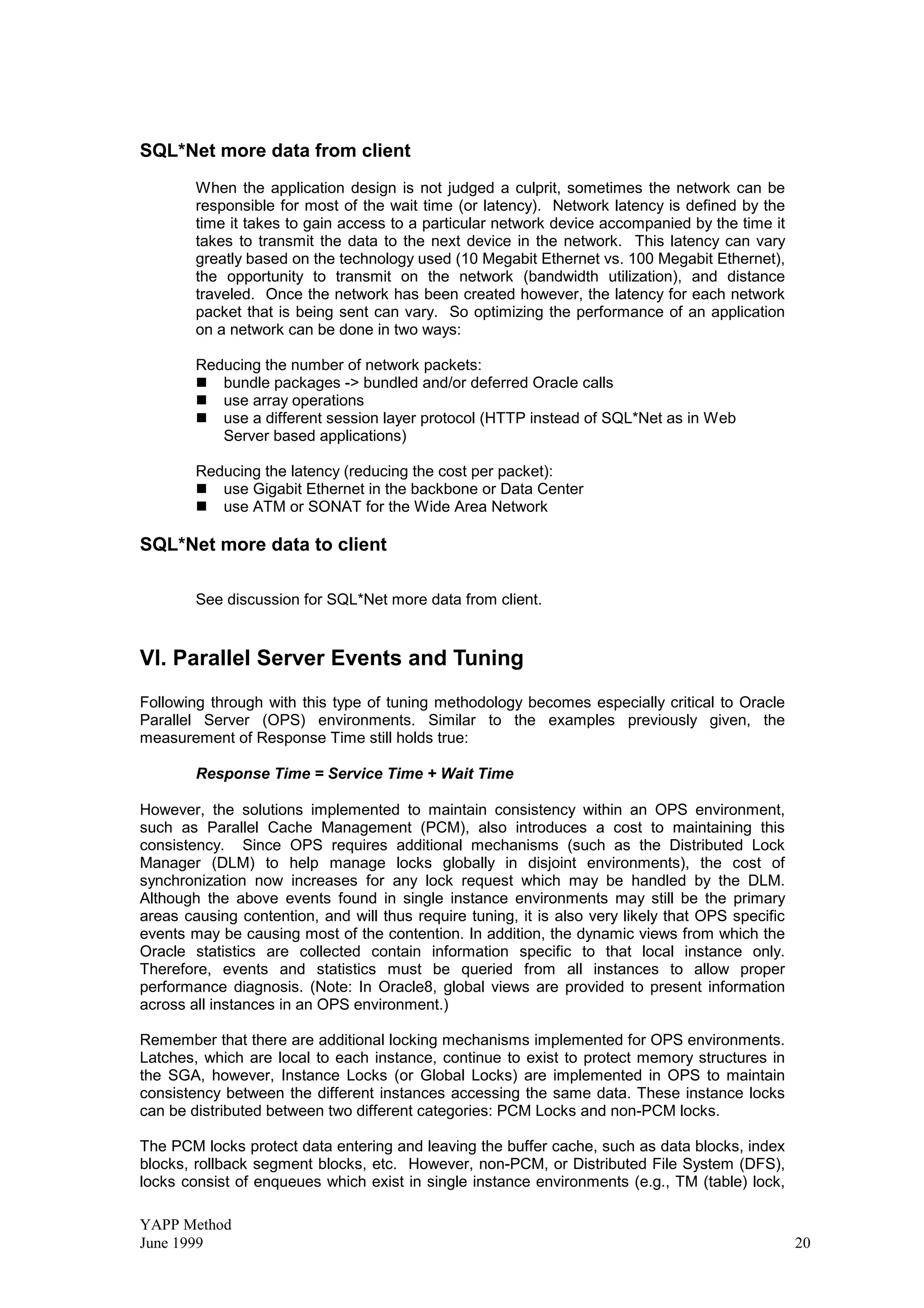
From these statistics, the percentage of parses vs. executes can be calculated (parse
count/execute count). If this ratio is higher than 20%, consider the following:
• ensure the application is using bind variables. By using bind variables, it is
unnecessary to reparse SQL statements with new values before re-executing. It
is significantly better to use bind variables and parse the SQL statement once in
the program. This will also reduce the number of network packets and round trips
[This reason becomes less relevant with Oracle8 OCI.] It will also reduce
resource contention within the shared pool.
• if using Forms, make sure that Forms version 4.5 (or higher) is used
• if applications open/re-parse the same SQL statements and the value of ‘session
cursor cache hits' is low compared to the number of parses, it may be useful to
increase the number of cursor cache for the session. If no hit ratio improvement
results, lower this number to conserve memory and reduce cache maintenance
overhead.
• check pre-compiler programs on the number of open cursors that they can
support (default = 10 in some cases). Also check if programs are pre-compiled
with release_cursors = NO and hold_cursors = YES
recursive cpu usage
This includes the amount of CPU used for executing row cache statements (data
dictionary lookup) and PL/SQL programs, etc. If recursive cpu usage is high, relative to
the total CPU, check for the following:
• determine if much PL/SQL code (triggers, functions, procedures, packages) is
executed. Stored PL/SQL code always runs under a recursive session, so it is
reflected in recursive CPU time. Consider optimizing any SQL coded within those
program units. This activity can be determined by querying V$SQL.
• examine the size of the shared pool and its usage. Possibly, increase the
SHARED_POOL_SIZE. This can be determined by monitoring V$SQL and
V$SGASTAT.
• set ROW_CACHE_CURSORS. This is similar to session cached cursors and
should be set to a value around 100. Since there are only some 85 distinct data
dictionary SQL statements executed by the server processes, higher values will
have no effect.
Other CPU
This composes of CPU time that will be used for tasks such as looking up buffers,
fetching rows or index keys, etc. Generally “other” CPU should represent the highest
percentage of CPU time out of the total CPU time used. Also look in v$sqlarea2
/v$sql
2
It is better to query from V$SQL since V$SQLAREA is a GROUP BY of statements in the
shared pool while V$SQL does not GROUP the statements. Some of the V$ views have to
take out relevant latches to obtain the data to reply to queries. This is notably so for views

11. YAPP Method
June 1999 11
to find SQL statements that have a high number of buffer_gets per execution and/or a
high number of physical reads per execution. Investigation of these gets (especially the
first) will help to reduce the remaining or “other” CPU time.
With the following SQL statement, find the overall CPU usage:
select a.value “Total CPU”,
b.value “Parse CPU”,
c.value “Recursive CPU”,
a.value - b.value - c.value “Other”
from v$sysstat a, v$sysstat b, v$sysstat c
where a.name = ‘CPU used by this session’
and b.name = ‘parse CPU time’
and c.name = ‘recursive CPU’;
Note: the descriptors in v$sysstat may change between versions!
The following SQL statement will show the CPU usage per session:
select distinct a.sid, a.value “Total CPU”,
b.value “Parse CPU”,
c.value “Recursive CPU”,
a.value - b.value - c.value “Other CPU”
from v$sesstat a, v$sesstat b, v$sesstat c
where a.statistic# = 12
and b.statistic# = 150
and c.statistic# = 8
Note: the descriptors in v$sysstat may change between versions!
Remember that fixing the CPU time may/will help to improve the throughput (depending on the
application profile).
V. Breaking Down Wait Time
If wait time is the largest contributor to total response time, decompose it into detailed
segments to further understand the problem.
To correctly identify the events contributing the highest amounts of wait time, query the view
V$SYSTEM_EVENT and order the events by time_waited:
select *
from v$system_event
where event not in (‘pmon timer’, ‘smon timer’, ‘rdbms ipc
message’, ‘parallel dequeue wait’, ‘virtual circuit’, ‘SQL*Net
message from client’, ‘client message’, ‘NULL event’) order by
time_waited;
Note: not a complete list of events to ignore (see time waited section above)
The output from V$SYSTEM_EVENT can be ordered to show the events that are the greatest
contributors to the amount of time waited. Utlbstat/utlestat will also generate a report.txt
file with similar output. Refer to the Oracle8 Reference Guide, Appendix A for more
information on when and how a particular event is used. From the event descriptions,
appropriate actions can then be taken to correct any performance problems identified.
However for the purpose of this paper, the following list represents the primary events that
usually contribute the greatest amount of wait time.
against the library cache and SQL area. It is generally advisable to be selective about what
SQL is issued against these views. In particular use of V$SQLAREA can place a great load on
the library cache latches.

12. YAPP Method
June 1999 12
buffer busy waits
This event is caused by:
• multiple sessions requesting the same block (i.e., one or more sessions are waiting
for a process to read the requested block into the buffer cache)
• multiple sessions waiting for a change to complete for the same block (only one
process at a time can write to the block, so other processes have to wait for that
buffer to become available)
If buffer busy waits is high, determine which blocks are being accessed concurrently and if
the blocks are being read or changed through V$SESSION_WAIT and V$WAITSTAT.
V$SESSION_WAIT will show the file#, block# and id (where id represents the status of
the buffer busy wait event).
• file# - data file number containing the block being read
• block# - block number being waited on
• id - buffer busy wait event:
• 1013/1014 - block is being read by another session
• 1012/1016 - block is being modified
V$WAITSTAT will show the block classes and the number of times waited for each.
Different actions may be taken for each block class to alleviate contention. Tuning
priorities should be oriented toward the classes that contribute the highest wait time
percentage.
segment header waits
Each segment has one segment header block. There are basically two types of
segments -- data and index. The following is a brief discussion on causes for
segment header blocks based on the data structures they contain:
• Problem: A high insert rate on a table with insufficient transaction free lists results
in a bottleneck.
• Solution: Increase free list groups. For databases running in exclusive mode,
this recommendation may also circumvent the issue of a small block size
constraining the number of available free lists.
• Problem: Under heavy insert activity, a table’s High Water Mark (HWM) is
constantly updated. This may be due to running out of blocks on the free lists and
need to replenish it by allocating new blocks. The default value for incrementing
the HWM is 5, which may be insufficient on a busy system or for the average
insert size.
• Solution: This value can be increased up to 255 through the undocumented
init.ora parameter, _BUMP_HIGHWATER_MARK_COUNT. Caution: this parameter
determines how many blocks to allocate per free list when bumping up the HWM.
Therefore, this can grow a table very quickly if it has a high number of free lists.
For example, if there are 100 free lists and
_bump_highwater_mark_count=100, then this may quickly add up to 10000
free blocks to the segment.
• Problem: Constantly inserting new entries into the extent map within the segment
header because extent sizes are too small.
• Solution: Increase the size of each extent. Although ORACLE7 release 7.3
allows an object to have unlimited extents, it is better to have a small number of
very large extents than to have a large number of small extents.
Data block waits

13. YAPP Method
June 1999 13
The data block class is used to store data (index or table data). Here are some
reasons for data block waits:
• Problem: multiple sessions could be requesting the same block from disk (this
could actually happen for each block class). Only one session will do the read
from disk, and the other sessions will be waiting for the block to be placed into the
buffer cache. The other sessions will be waiting on the buffer busy wait event
(1014).
• Solution: the buffer cache may be too small to keep the current working set in
memory. Enlarging the buffer cache (db_block_buffers) can help. Another
option is to use buffer pools to reduce the number of buffers an object can occupy
in the buffer cache. For example, we may effectively limit the number of buffers
that a randomly accessed large table can occupy in the buffer cache by placing it
in the recycle pool.
• Problem: multiple sessions are going after rows in the same block because it
contains so many rows.
• Solution: reduce the number of rows per block (i.e., modify pctfree/pctused
settings). This is a space for time tradeoff. The table will use more space, but
‘buffer busy waits’ will be reduced.
• Problem: multiple sessions are trying to insert into the same block because there
is only one free list (or insufficient free lists).
• Solution: adding multiple free lists to the object will increase the number of heads
of free lists, thus the contention point can be distributed over the free lists,
reducing the number of buffer busy waits.
Free list block waits
This statistic measures contention for “free list group” blocks. Some documentation
and tuning scripts claim that waits on this block class indicate that the number of free
lists need to be increased for some objects. Most databases that run in exclusive
mode see zero waits on this block class because their DBAs do not create objects
with free list groups. Otherwise, the reasons and solutions for free list block waits are
similar to those of segment header waits. See that section for details.
Identifying block waits by file
X$KCBFWAIT shows a count of buffer busy waits per file. The indx column represents the
file id number - 1. So this view can be queried to determine which file has a high number
of buffer busy waits.
select indx+1 fileno, count, time
from x$kcbfwait
where time != 0 or count 0
order by time;
If the file with highest wait time is known, find the objects that belong to that file:
select file_id, segment_name, segment_type, freelists,
freelist_groups, pctfree, pctused
from dba_extents
where file_id = fileno;
db file scattered read
This wait event usually indicates some type of multi-block I/O operation (full table scans or
fast full index scans in Oracle 7.3 and higher). The number of data blocks read per I/O
operation is determined by the init.ora parameter db_file_multiblock_read_count
(which can be changed dynamically in Oracle 7.3).
Check with v$filestat to see which files have done scans:
select file#, phyrds, phyblkrd, readtim
from v$filestat
where phyrds != phyblkrd;

14. YAPP Method
June 1999 14
If phyrds is close to phyblkrd then single block reads are occurring. If that is not the case,
full scans or range scans are happening on that file.
To reduce the cost of a db file scattered read, check the file placement on each disk, the
number of disks, and the stripe size per disk (this should be
2*db_file_multiblock_read_count).
To reduce the amount of a db file scattered read, check for missing indexes on the object
where the scan is happening or check the SQL statement that is executing the scan.
db file sequential read
This event occurs for single block reads (like index lookup). The normal way to reduce
this event is to examine the amount and cost of the I/Os that are preformed. One can
normally reduce the amount of I/Os and make each I/O faster.
• Reducing the amount of I/Os
To achieve this, a number of things can be done:
• increase db_block_buffers
It is likely that the buffer cache is too small. In today’s market, memory is getting
cheaper and systems with a large amount of memory are becoming more
common. Even Very Large Memory (VLM) systems are available. Increasing the
number of buffers will have a positive effect on the buffer cache hit ratio. It is
important to realize that even a small increase in the buffer cache hit ratio can
have a dramatic effect if the buffer cache is large.
• reduce physical reads per execute for SQL statements
In the introduction, it was stated that tuning SQL could have a big impact on the
overall performance of the system. One of the biggest wait components of the
SQL statement execution is the I/O. Finding the SQL statement with the most
reads per execution is a good start:
select disk_reads, executions, disk_reads/executions,
sql_text
from v$sql
where executions != 0
order by 3;
Once the SQL statement with the highest reads per execution has been identified,
it is good to have a quick look at the number of executions (or the total number of
reads that the SQL statement has done). It is more important to check that the
SQL statement being tuned is significant to the application instead of being one
that is executed only once (at night for example in a batch job). It is also
worthwhile to use the same query to identify the SQL statements that are
executed most:
select disk_reads, executions, disk_reads/executions,
sql_text
from v$sql
where executions != 0
order by 2;
Incremental improvements on a query executed many times can provide
significant performance gains. In either case, tuning SQL statements is a skill in
itself. This paper will only help in identifying the SQL statement that needs to be
fixed not how it should be fixed.
Using the 'CACHE' option
A table can be created with or modified to use the CACHE option. Buffers
retrieved for this object through a Full Table Scan (FTS) will be placed on the

15. YAPP Method
June 1999 15
Most Recently Used end of the buffer cache LRU list (replacing the normal
behavior of placing those buffers at the Least Recently Used (LRU) end of the
LRU list)
Choose the tables to cache wisely. Sometimes caching the smallest table may be
best the thing to do. The problem is that random access to a large table using the
CACHE option may force out blocks from a smaller table that are less frequently
accessed. Another example is the sequential write to a history type of table. All
the writes to that table may end up in the cache, forcing out older blocks from
other objects.
• buffer pools (Oracle8).
In Oracle8, we can assign objects to buffer pools, and each buffer pool can have
a different replacement policy, a certain number of buffers, and a number of LRU
latches. The recycle replacement policy may reduce the number of buffers that
an object can occupy. For example, a randomly accessed large table can slowly
take over the buffer cache, by squeezing out the less frequently used blocks of
other objects. A solution would be to assign the large object to a small recycle
buffer pool. This leaves the rest of the buffer cache for the other objects and
improves the buffer cache hit ratio.
• Reducing the cost of I/Os
The following can be done:
• use faster disks/controllers
Faster disks can make a big difference. See the example earlier in this paper.
Do not be fooled by disks with large caches, since it can appear that all operations
are coming from the cache. However, with a large OLTP application, writes to
disk must eventually occur. If the physical writes are slow, they could delay the
write into the disk cache (possibly from a need to find room or write out a dirty
block). Also, having one 9GB drive (running at 5400 RPM) is not necessarily
better than two 4GB drives (running at 4500 RPM). The total number of reads
and writes that can be done is the most important factor to consider. If each disk
can complete a read or write in around 100 I/Os per second, 2 slower RPM drives
would be a more optimal solution by doubling the I/Os per second.
• check the wait time for each disk
Find the disks with the highest wait time and check to see what objects reside on
that disk. It may be necessary to physically redistribute the data.
• find the number of I/O per filesystem/logical volume, disk, controller
Uneven distribution of I/O among filesystems, disks and controllers can be
identified by mapping the I/O statistics gathered from sar and V$FILESTAT to
controllers, disks, logical volumes and filesystems.
• use better stripe sizes or stripe widths
• find the average read time per file
• use more disks to stripe a file over
• find disks with the highest read time
In order to determine which file may be causing a problem for I/O use V$FILESTAT.
Examine the ratio of readtim (amount of time spent reading) and phyrds (total number of
reads) per file:
select file#, readtim, phyrds, readtim/phyrds from v$filestat
order by 4;
Look at the file with the highest read percentage out of the total reads and the highest
read times. If the average cost per I/O is high this may indicate a need to increase the
stripe width or the total number of disks involved in striping. Also look at the total number
of I/Os per transaction, then how many concurrent transactions are running, for example:

16. YAPP Method
June 1999 16
If each transaction requires 2 reads + 1 write and the expectation is to perform
1000 transactions per second, this calculation requires that the system actually
process 3000 I/Os per second. Therefore, if one disk can perform 50-100 I/Os
per second, at least 60 disks will be needed (3000 divided by 50). Now if the
requirement doubles from 1000 transactions per second to 2000, it will be
necessary to double the number of disks. This, however, is often forgotten in the
real world.
Remember that it is important to get a sense of the scale needed to meet the requirement.
Also, plan for stress capacity. With 100 users, the I/O might be just fine, but if the number
of users is doubled, then the current disks and striping may no longer be sufficient. To
increase throughput, disks will need to be added!
free buffer waits
Free buffer waits may be caused by the session scanning a buffer cache LRU list for a
free buffer. If the dirty list is full, then a foreground process must wait for dirty buffers to be
written to disk. Or when a session scans too many buffers
(_db_block_max_scan_count in Oracle7), it is more likely that the dirty list is full, so
increasing _db_block_write_batch should be sufficient.
Check for the following statistics in v$sysstat and v$sesstat:
• free buffers inspected
The number of dirty and pinned buffers skipped before a free buffer is found.
• free buffers requested
The number of buffers requested to store data by all sessions.
• dirty buffers inspected
The number of dirty buffers (buffers that need to be flushed to disk before they
can be reused by sessions).
The following formula will calculate the average number of buffers that a session is
scanning at the end of an LRU to find a free buffer:
1 + (free buffers inspected/free buffers requested)
If this number is close to 1, it means a process can find a buffer on average very quickly.
If the number is very large, it normally means that a lot of Consistent Read (CR) buffers
are sitting at the end of the LRU (sometimes buffers are put at the end of the LRU so that
the hot buffers will stay at the top of the LRU).
Other interesting buffer cache statistics are:
• DBWR free buffers found
When the DBWR was scanning for buffers to write, it found this number of free
buffers (buffers that did not need to be flushed).
• DBWR dirty buffers found
When the DBWR was scanning for buffers to write, it found this number of dirty
buffers (buffers that did need to be flushed).
• Physical writes
The number of dirty blocks flushed to disk by the DBWR.
• Write requests
The number of batches of dirty buffers flushed to disk.
latch free
With a high number of latch free waits, it is important to determine which latch is being
requested most. When the bottleneck is a single latch (single threaded), increasing the
spin count can help in multiple CPU (SMP) machines. In this case, it is ‘cheaper’ to spin
the CPU than to pay the cost to have a process sleep. However, if a system is already
CPU-bound, increasing spin_count may worsen the situation.

17. YAPP Method
June 1999 17
Two of the most highly contended latches are the shared pool latch and the library cache
latch. Each of these latches can be held for a long time so if there is contention, a low
value for the spin_count variable can cause processes to sleep unnecessarily. There
can also be a great deal of contention for the redo allocation latch. The redo allocation
latch is used for allocating space in the log buffer when foregrounds need to write redo
records
All of these latches are potential points of contention. In case of the library cache latches
and shared pool latch, the number of latch gets occurring is influenced directly by the
amount of activity in the shared pool, especially parse operations. Anything that can
minimize the number of latch gets and indeed the amount of activity in the shared pool is
helpful to both performance and scalability.
The event latch free is equal to the SUM of sleeps in v$latch.
• First use V$LATCH to determine the latch with the highest sleep count:
select name, sleeps
from v$latch
order by sleeps;
• Since V$LATCH only shows the parent latch, check V$LATCH_CHILDREN to
determine which child latch (if any) has the most contention:
select name, sleeps
from v$latch_children
where name = latch name
and sleeps minimum base
order by sleeps;
• Depending on the latch type many different changes can be made:
• Shared pool latch Library cache latch
Every time an application makes a parse call for a SQL statement, and the
parsed representation of the statement is not in the shared SQL area, Oracle
parses and allocates space in the library cache. The shared pool and library
cache latches protect these operations. Once the SQL area becomes
fragmented and available memory is reduced, the single-threaded shared
pool latch may become a bottleneck. Contention for these latches can be
achieved by increasing sharing of SQL, and reducing parsing by keeping
cursors open between executions.
• cache buffer hash chain latch
Each hash chain latch protects a hash chain comprised of a number of buffer
headers, which in turn point to the buffer itself. This latch is acquired every
time when a buffer is queried or updated. The number of latches defaults to
prime(0.25 * db_block_buffers). There could be a large number of
latches, so it is important to add the clause “where sleeps some
number n” to filter out most of the latches. Find the latch with the highest
sleep. Then find the buffers that are protected by that latch:
select hladdr, dbafil, dbablk
from x$bh b, v$latch_children l, (select max(sleeps)
maxsleeps from v$latch_children where type = 11)
where type = 11 –- check v$latchnames for cache buffer -
-- hash chain latches
and l.addr = hladdr
and sleeps = maxsleeps;
Note: please use the column FILE# instead of DBAFIL in Oracle8.
When the dbafil and dbablk values are found, check dba_extents to see
what the object name and type is:

18. YAPP Method
June 1999 18
select segment_name, segment_type
from dba_extents
where file = file
and block between block_id and block_id + blocks - 1;
log file sync
Log file sync happens at commit time when a foreground is waiting for LGWR. Generally the
time should be less than 0.2 - 0.5 seconds per wait
3
.
This event is measured at the session level. The session is waiting for the log writer
(LGWR) to flush redo to disk. Inside the log writer, a number of other potential waits will
happen:
log file parallel write (event)
redo writer latching time (statistic)
Find the average redo write size:
(Redo blocks written/redo writes) * 512
4
bytes (usually) = avg. redo write size
If there is significant redo generation but the average write size is small, check for
write back caches at the disk level or disk array level. Caching the redo writes may be
dangerous (and may lead to possible data corruption), but it could also negatively
affect the performance of the whole system. If the LGWR process is too active, it
could cause too much redo latch contention. Another reason for a small average
redo write size could be that LWGR is unable to piggyback many commits. The
whole system may not be very busy resulting in LGWR waking up immediately (when
posted) and writing the redo for a session. This means that the next session may
have to wait for this write to complete before its redo will be written. The maximum
I/O size for the redo writer is also port specific. The normal values can range from
64K to 128K.
Striping the log file may help in this case. A recommended stripe size (or stripe width)
is 16K. Also sizing the redo log buffer correctly is important. To calculate an
approximate size use:
(3* ( (redo size/(user commits + user rollbacks)) * transaction commits per second))/2
5
enqueue
When this event shows up in v$system_event, also check x$ksqst to see what enqueue
type is causing the waits:
select *
from x$ksqst6
3
Before 8.0.4, there was a problem where LGWR was not always posting the correct foreground
processes. As a result, some foreground processes were timing out and therefore accrued a response
time of at least one second (as the timeout value for this event is 1 second). If this is found, contact
Oracle Support for the proper patch.
4
The redo block size depends on the physical block size for the port. For most ports this is 512 bytes,
but for some ports this is actually a larger value (2K or 4K). dbfsize redo log file will tell what the
block size is.
5
Multiply by 1.5 since LGWR will start to write the redo buffer when it becomes 2/3 full or when a
foreground or DBWR will post LGWR.
6
x$ksqst is an internal view. It can change without any notice or may even be dropped in a future
release. So do not depend on it.

19. YAPP Method
June 1999 19
where ksqstget != 0
order by ksqstget;
This will show gets and waits for all enqueue types. Also v$sysstat/v$sesstat shows
some interesting information:
• enqueue gets
The number of enqueue “get” operations that are performed. For example getting
the ST lock will count as an enqueue get.
• enqueue converts
The number of enqueue convert operations that are performed. For example,
converting an enqueue from S (shared) mode to X (exclusive) mode.
• enqueue releases
Most enqueues that are obtained are then released. This means the number of
conversions will be minimal or non-existent on most systems.
• enqueue waits
The number of times that a session tried to get an enqueue but could not right
away (this is true for enqueue gets and enqueue conversions). Some tuning
sources state that if the enqueue waits are high, then enqueue_resources
need to be increased. This is incorrect. Waits just indicate that an enqueue could
not be granted. If enqueue_resources are depleted, an appropriate message
indicating the need to increase resources is returned immediately.
• enqueue deadlocks
Indicates the number of deadlocks detected for the session or the number of
ORA-60 errors returned to the session.
• enqueue timeouts
If an enqueue could not be granted, it means that the session will have to wait
(enqueue waits), and within the wait, there can be several timeouts.
Look in v$lock or v$session_wait to see what the enqueue sessions are currently
waiting on:
select * from v$session_wait where event = ‘enqueue’;
Examples of most common enqueue types that will show in the above queries
CF - Control File Enqueue
SQ - Sequence Enqueue
ST - Space Management Transaction
TM - DML enqueue
TS - Table Space enqueue
TX - Transaction enqueue
mode 6 = row level lock
mode 4 = not enough ITL entries in object (that could be index or table)
(Join v$session_wait with v$session with v$sql to find the current SQL statement and
object for this session).
write complete waits
When a buffer is being written, it cannot change until the buffer is flushed to disk. The
most common reason for this to happen is frequent checkpointing. Normally a hot buffer
will stay at the Most Recently Used end of the LRU and the chance that it will be written is
small. Checkpointing occurs normally due to:
„small redo log files
„default setting of log_checkpoint_interval

20. YAPP Method
June 1999 20
SQL*Net more data from client
When the application design is not judged a culprit, sometimes the network can be
responsible for most of the wait time (or latency). Network latency is defined by the
time it takes to gain access to a particular network device accompanied by the time it
takes to transmit the data to the next device in the network. This latency can vary
greatly based on the technology used (10 Megabit Ethernet vs. 100 Megabit Ethernet),
the opportunity to transmit on the network (bandwidth utilization), and distance
traveled. Once the network has been created however, the latency for each network
packet that is being sent can vary. So optimizing the performance of an application
on a network can be done in two ways:
Reducing the number of network packets:
„bundle packages - bundled and/or deferred Oracle calls
„use array operations
„use a different session layer protocol (HTTP instead of SQL*Net as in Web
Server based applications)
Reducing the latency (reducing the cost per packet):
„use Gigabit Ethernet in the backbone or Data Center
„use ATM or SONAT for the Wide Area Network
SQL*Net more data to client
See discussion for SQL*Net more data from client.
VI. Parallel Server Events and Tuning
Following through with this type of tuning methodology becomes especially critical to Oracle
Parallel Server (OPS) environments. Similar to the examples previously given, the
measurement of Response Time still holds true:
Response Time = Service Time + Wait Time
However, the solutions implemented to maintain consistency within an OPS environment,
such as Parallel Cache Management (PCM), also introduces a cost to maintaining this
consistency. Since OPS requires additional mechanisms (such as the Distributed Lock
Manager (DLM) to help manage locks globally in disjoint environments), the cost of
synchronization now increases for any lock request which may be handled by the DLM.
Although the above events found in single instance environments may still be the primary
areas causing contention, and will thus require tuning, it is also very likely that OPS specific
events may be causing most of the contention. In addition, the dynamic views from which the
Oracle statistics are collected contain information specific to that local instance only.
Therefore, events and statistics must be queried from all instances to allow proper
performance diagnosis. (Note: In Oracle8, global views are provided to present information
across all instances in an OPS environment.)
Remember that there are additional locking mechanisms implemented for OPS environments.
Latches, which are local to each instance, continue to exist to protect memory structures in
the SGA, however, Instance Locks (or Global Locks) are implemented in OPS to maintain
consistency between the different instances accessing the same data. These instance locks
can be distributed between two different categories: PCM Locks and non-PCM locks.
The PCM locks protect data entering and leaving the buffer cache, such as data blocks, index
blocks, rollback segment blocks, etc. However, non-PCM, or Distributed File System (DFS),
locks consist of enqueues which exist in single instance environments (e.g., TM (table) lock,

21. YAPP Method
June 1999 21
TX (transaction) lock, etc.) and locks which are unique to OPS (e.g., SC (system commit
number) lock). In Oracle7, the non-PCM locks, which exist as local enqueues for single
instance environments but become global for OPS, are identified by events that begin with
“DFS enqueue.” Non-PCM locks that are unique to parallel server environments are identified
by events that begin with “DFS lock
PCM Lock Events
lock element clean up - indicates a process is waiting on getting a lock element (trying to get
a block). This usually indicates pinging (remote requests from another instance for a block).
Problems related to block pings can use the following method to determine which objects and
blocks are causing the highest percentage of pinging, as well as the type (false, soft, or hard)
and number of pings.
Identify which blocks, along with the corresponding block classes, are being pinged and which
object they are associated with. Depending on the block class and object take the appropriate
action such as adjusting the corresponding GC_ parameter, adding free list groups, etc.
Note: In Oracle7, V$FILE_PING and V$PING do not correctly report all the ping
statistics! These views only count conversions down to N (Null) where it should actually count
all down conversions from X (Exclusive), such as X-S, X-SSX and X-N. Since an X lock is
held for writes, any down conversions from exclusive mode will force dirty blocks in the cache
covered by the lock, to be written to disk.
See the following chart for the areas where V$PING misses counts:
Type of Convert Could this cause a write? Counted by V$PING?
X - N Yes Yes
X - SSX Yes No
X - S Yes No
S - N No Yes
The ping count for these views are fixed in Oracle8, but be aware that these statistics in
Oracle7 may not be accurate! For Oracle7, V$LOCK_ACTIVITY is one of the views that can
indicate how much pinging is taking place within an instance. Through this view, it is possible
to explicitly count the various PCM Lock converts that are taking place.
Checking frequency of PCM Lock Conversion
X to NULL = instance gave up block at request of another instance
X to S = instance shared block with another instance
X to SSX = instance shared block with another instance
NULL to S = instance requested a block from another instance
S to X = instance requested a block from another instance
select (value/(a.counter + b.counter + c.counter) - 1)/
(value/(a.counter + b.counter + c.counter)) Rate
from v$sysstat,
v$lock_activity a,
v$lock_activity b,
v$lock_activity c
where a.from_val = 'X'
and a.to_val = 'NULL'
and b.from_val = 'X'
and b.to_val = 'S'
and c.from_val = 'X'
and c.to_val = 'SSX';

22. YAPP Method
June 1999 22
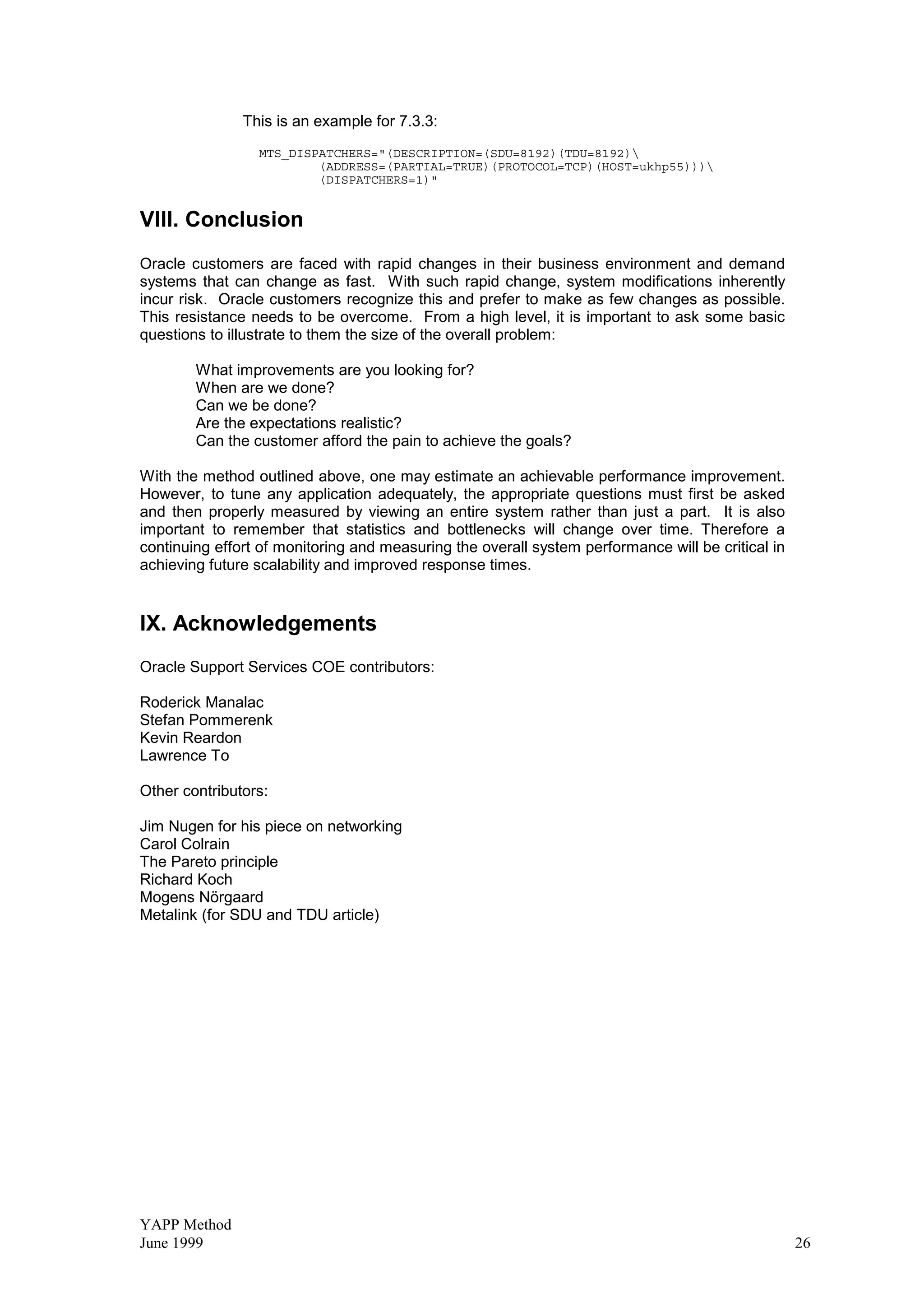
It is also feasible to use the event DBWR cross instance writes from V$SYSSTAT to
determine the number of writes taking place due to ‘pings’. In order to obtain a percentage of
writes done for remote requests compared to total writes done for an instance:
% of writes due to pings = DBWR cross instance writes/physical writes
select y.value All Writes,
z.value Ping Writes,
z.value/y.value “Pings Rate
from v$sysstat y,
v$sysstat z
where z.name = 'DBWR cross instance writes'
and y.name = 'physical writes';
Note: Ping Rate value measures FALSE pinging activity ( 1 indicates false pings, 1
indicates soft pings)
To identify blocks that have a high ping rate and their corresponding class, query the view
V$BH. If PCM lock adjustments are needed, then modify the appropriate Global Cache (GC_)
parameter that corresponds to the particular block class.
Block Class Meaning GC Parameter
1 Data Blocks GC_DB_LOCKS,
Contains data from indexes or tables GC_FILES_TO_LOCKS
2 Sort Blocks - Contains data from on
disk sorts and temporary table locks. [no PCM locks needed]
3 Save Undo Blocks GC_SAVE_ROLLBACK_LOCKS
4 Segment Header Blocks GC_SEGMENTS
5 Save Undo Header Blocks GC_TABLESPACES
6 Free List Group Blocks GC_FREELIST_GROUPS
7 System undo Header Block GC_ROLLBACK_SEGMENTS
System Undo Blocks GC_ROLLBACK_LOCKS
Total number of pings (XNC - X to Null count) for each block where XNC !=0
Note: Once a block completely exits the cache (i.e., there are no versions of the block left in
the buffer cache), the XNC count gets reset to 0. Therefore it will be important to monitor this
view during regular intervals to obtain a better indication of blocks which are pinged
excessively.
Pings per file / block
select file#, block#, class#, status .xnc count
from v$bh a
where b.xnc!=0 and status in (‘XCUR’, ‘SCUR’)
order by xnc, file#, block#;
Once the file and blocks causing the highest amount of contention are identified, determine
the corresponding object and how that object is currently being accessed by querying V$SQL.
To determine the corresponding object name and type:
select segment_name, segment_type
from dba_extents
where file_id=file#
and block# between block_id and block_id + blocks – 1;
To determine the type of SQL statements being executed:

23. YAPP Method
June 1999 23
select sql_text, executions,
decode(command_type, 2, ‘INSERT’, 3, ‘SELECT’, 6, ‘UPDATE’, 7,
‘DELETE’, ‘OTHER’ )
from v$sql ;
Note: For additional information on command types, please reference the Oracle Server
Reference Manual.
lock element waits - indicates a process is waiting on a lock element convert (for example,
another process within the same instance is currently getting the lock)
This can be caused by either not having enough locks (possibly false pinging) or processes
requesting the same set of blocks.
Note: For OPS there is a hint in the optimizer when getting locks for unique indexes, so that if
1 row is being changed, the lock is gotten directly in XCUR mode. However, if it is getting two
rows or more it is first gotten in SCUR then upgraded to XCUR.
Non PCM Lock Events
DFS enqueue lock acquisition
DFS lock release
DFS lock convert
DFS lock acquisition
These events indicate that a process is waiting on acquiring or converting a global lock.
Depending on the lock type and the corresponding identifiers different actions can be taken to
tune this piece appropriately. In order to determine the enqueues that have a high number of
waits, query the view X$KSQST (also described in section IV below).
select * from x$ksqst where ksqstget != 0;
Depending on the enqueue type that shows a high number of waits, appropriate action can
then be taken. This will show the type, the number of gets, and the number of waits. For
example high TS and ST waits may indicate a need to check and/or increase extent sizes. TM
waits and gets represents table locks. For this issue, consider disabling table locks. ST waits
indicates space management tasks such as coalescing free space, cleaning up temporary
segments, or allocating and de-allocating extents.

24. YAPP Method
June 1999 24
VII. Additional Discussions and Examples
1) Logging on and off
The log on and log off operations are costly since a login must get a unique session id from
the AUDSESS$ sequence number every time. In the example of sessions continuously logging
on and off, the recursive CPU and wait time for access to the block containing AUDSESS$
would be high. Since the cache size for AUDSESS$ is only 20, increasing this value can help
the performance of login operations. For OPS environments, the cost is even greater if there
are multiple processes concurrently logging onto the different instances. If multiple OPS
instances are requesting a single block containing AUDSESS$, this will cause additional lock
and pinging overhead.
2) Networks
Inband-breaks:
Inband breaks are used over TCP and IPC protocols, which check for a pending Control-C on
an existing connection. This can severely affect the performance of long running queries when
issued over TCP/IP, if this polling is done excessively. This is specifically for platforms like AIX
or NT, which use in-band breaks in Oracle7 (NT always uses inband breaks), when out-of-
band breaks (OOB) can’t be negotiated. Where possible, Oracle generally uses out-of-band
breaks. The undocumented sqlnet.ora parameter BREAK_POLL_SKIP needs to be set to a
very high value (like 10000000000) to reduce the number of breaks. However, increasing the
parameter will in turn lead to “hanging” queries when a Control-C is issued to interrupt the
processing.
SQL*Net packet size:
Is it possible that SQL*Net’s number of small packets is causing network performance
problem? The answer is in RFC 896. To avoid congestion on a network by many small
packets, a solution was proposed called the ‘Nagle algorithm’. This algorithm tells TCP to wait
to send data (until a time out period) if the total amount of data to be sent is less then its
buffers can hold. For real-time applications that depend on data being sent as quickly as
possible, the Nagle algorithm should be disabled. Unfortunately, some versions of SQL*Net
TCP/IP are subject to this algorithm. There is a fix in 7.2.3 (bug 475453) and generic solution
in 7.3.3 upward (bug 449089).
Consider the network Maximum Transmission Unit (MTU) when setting the Session Data Unit
(SDU). Most of the time setting the SDU will not be necessary as RFC 1191 (Path MTU
Discovery) is commonly used in most TCP’s. If it is not, then fragmentation and reassembling
of packets have a chance to occur at the IP level. This is caused by the MTU sizes differing
for each network traversed so the packets must broken into the smallest size and transmitted
over the small MTU network, being reassembled at the receiving end.
For the most part, the best way to solve network problems is to create an application that uses
less packets, or use an application technology that is designed to use less packets (like Web
based applications that use HTTP).
Some hints on improving performance:
tcp.nodelay = true in the sqlnet.ora file on the client and the server side (for 2.2
and 2.3 of SQL*Net). This will force TCP to send the packet (set the push bit) and not
wait.
In SQL*Net v2.3, change the Session Data Unit (SDU) to multiples of the MTU. It is
will also be necessary to make this change on the server side (as the SDU is
negotiated during the initial database connect and the smallest is then used). If the

25. YAPP Method
June 1999 25
SDU is set in multiples of the underlying network packet size, then you may also
achieve some additional performance gain.
How to specify the SDU and TDU:
Packet Sizes:
SQL*Net allows limited control over the packet sizes via the two parameters Session Data
Unit (SDU) and Transmission Data Unit (TDU). These control the sizes of the 'Session' and
'Transport' layer buffers respectively.
Prior to 7.3, SDU and TDU are limited to 2k.
In 7.3 onwards these are tunable above 2k.
SDU size is tunable (up to 32K) from Oracle7 release 7.3 onwards.
For example, if configuring for a pure Ethernet network, it is possible to set the above
buffers to 8 times the size that can be transmitted inside an Ethernet frame. Do to this, in the
in TNSNAMES.ORA the following sizes can be set:
alias= (DESCRIPTION=
(SDU=8192) **** service layer buffer size
(TDU=8192) **** transport layer size
(ADDRESS= (PROTOCOL=tcp) (PORT=2010) (HOST=abc))
(CONNECT_DATA= (SID=db3))
)
It is possible to set TDU different to SDU, but there is no reason to do this. For example, with
TDU=1024 and SDU=1536, 512 and then 1024 bytes of data will be sent to the transport. With
TDU=2048 and SDU=1536, 1536 bytes of data will be sent to the transport.
SDU / TDU Configuration:
To configure the TDU / SDU sizes to work properly for a particular network, ensure that the
TDU/SDU figures appear in all the relevant places. Here are some examples for the 3 main
locations:
TNSNAMES.ORA: The parameters must appear in the DESCRIPTION clause.
UKHP55_V732.UK.ORACLE.COM =
(DESCRIPTION =
(SDU=8192) **** Calls to this alias will
(TDU=8192) **** try to put 8K into packets.
(ADDRESS = (COMMUNITY = TCP.uk.oracle.com)
(PROTOCOL = TCP)
(HOST = ukhp55.uk.oracle.com)
(PORT = 1521)
)
(CONNECT_DATA = (SID = V7323))
)
LISTENER.ORA: The parameters must appear in the SID_DESC clause.
SID_LIST_LISTENER =
(SID_LIST =
(SID_DESC =
(SDU = 8192) **** Connects to this SID will
(TDU = 8192) **** try to use put 8K into packets.
(SID_NAME = V7323)
(ORACLE_HOME = /oracle/product/7.3.2.3)
)
(SID_DESC = **** This one will default
(SID_NAME = V723) **** (generally to 2K)
(ORACLE_HOME = /oracle/product/7.2.3)
)
)
INIT(SID).ORA: For MTS you cannot force TDU/SDU sizes until 7.3.3.
See Note:44693.1 for a full description of the MTS
configuration Parameter: MTS_DISPATCHERS.

26. YAPP Method
June 1999 26
This is an example for 7.3.3:
MTS_DISPATCHERS=(DESCRIPTION=(SDU=8192)(TDU=8192)
(ADDRESS=(PARTIAL=TRUE)(PROTOCOL=TCP)(HOST=ukhp55)))
(DISPATCHERS=1)
VIII. Conclusion
Oracle customers are faced with rapid changes in their business environment and demand
systems that can change as fast. With such rapid change, system modifications inherently
incur risk. Oracle customers recognize this and prefer to make as few changes as possible.
This resistance needs to be overcome. From a high level, it is important to ask some basic
questions to illustrate to them the size of the overall problem:
What improvements are you looking for?
When are we done?
Can we be done?
Are the expectations realistic?
Can the customer afford the pain to achieve the goals?
With the method outlined above, one may estimate an achievable performance improvement.
However, to tune any application adequately, the appropriate questions must first be asked
and then properly measured by viewing an entire system rather than just a part. It is also
important to remember that statistics and bottlenecks will change over time. Therefore a
continuing effort of monitoring and measuring the overall system performance will be critical in
achieving future scalability and improved response times.
IX. Acknowledgements
Oracle Support Services COE contributors:
Roderick Manalac
Stefan Pommerenk
Kevin Reardon
Lawrence To
Other contributors:
Jim Nugen for his piece on networking
Carol Colrain
The Pareto principle
Richard Koch
Mogens Nörgaard
Metalink (for SDU and TDU article)

27. YAPP Method
June 1999 27
Oracle Corporation
World Headquarters
500 Oracle Parkway
Redwood Shores, CA 94065
U.S.A.
Worldwide Inquiries:
+1.650.506.7000
Fax +1.650.506.7200
http://www.oracle.com/
Copyright © Oracle Corporation 1999
All Rights Reserved
This document is provided for informational purposes only, and
the information herein is subject to change without notice.
Please report any errors herein to Oracle Corporation. Oracle
Corporation does not provide any warranties covering and
specifically disclaims any liability in connection with this
document.
Oracle is a registered trademark, and Oracle7, Oracle8, Oracle8i,
SQL*Net, and Net8 are trademarks of Oracle Corporation.
All other company and product names mentioned are used for
identification purposes only and may be trademarks of their
respective owners.