Xu umn 0130_e_12193

1. Essays on Globalization and Economic Development A DISSERTATION SUBMITTED TO THE FACULTY OF THE GRADUATE SCHOOL OF THE UNIVERSITY OF MINNESOTA BY Nan Xu IN PARTIAL FULFILLMENT OF THE REQUIREMENTS FOR THE DEGREE OF Doctor of Philosophy Timothy J. Kehoe, Adviser Fabrizio Perri, Co-Adviser August, 2011

3. Acknowledgements I would like to thank my advisers Tim Kehoe and Fabrizio Perri for their con- tinued guidance and support through the project. They brought me to the

4. eld of international economics and taught me how to do serious economic research. I would also like to extend my thanks to Tom Holmes and Terry Roe for serving on my exam committee and providing helpful comments and suggestions during the early period of this project. I would like to thank Pu Chen, Yenan Hou, Jing Fang, and Dingming Liu for their helpful discussions. Many thanks also go to the participants of Trade and Development Workshop at Minnesota. Finally, I would like to express my deepest gratitude to my parents who make it possible. I also thank my wife Bai Jieru for making it happen. i

5. Dedication To Bai Jieru, for her unending love and support ii

6. Abstract This thesis investigates the role of globalization in economic development. This thesis consists of three essays. The

7. rst essay studies the role of resource reallocation and globalization in economic development for China. Recent literature on economic growth emphasizes the misallocation of resource at the micro level could reduce TFP at the macro level. Both structural transformation and globalization in China contribute to correct the misallocation of resources in China. Hence they could account for the remarkable growth experience of China. This paper develops a neoclassical growth model that emphasizes the role of structural transformation and international trade to account for the growth experience of China. I calibrate the model to match the data of China and show that the process of structural transformation in an open economy can generate growth rate of GDP comparable to those observed in China in the period 1991-2004. The second essay is a theoretical study of international trade and economic growth. I build an endogenous growth model with heterogeneous

8. rms. I

9. nd that trade liberalization can help reallocate resources to innovation and therefore promotes economic growth. The third essay reviews the literature of structural change and its implications for economic development. Developing countries started to develop from reallocating labor in agriculture to industrial production. This essay reviews iii

10. the two main mechanism to generate structural change in standard models of economic growth. Then I review the literature on the role of structural change in studying various issues in economic development. iv

11. Contents Acknowledgements i Dedication ii Abstract iii List of Tables viii List of Figures ix 1 Introduction 1 2 Reallocation, Globalization, and Economic Growth in China 5 2.1 Introduction . . . . . . . . . . . . . . . . . . . . . . . . . . . . . 5 2.1.1 Related Literature . . . . . . . . . . . . . . . . . . . . . 10 2.2 Empirical Evidence: The China Miracle . . . . . . . . . . . . . . 13 2.3 The Model . . . . . . . . . . . . . . . . . . . . . . . . . . . . . . 15 2.3.1 Household . . . . . . . . . . . . . . . . . . . . . . . . . . 16 2.3.2 Technologies . . . . . . . . . . . . . . . . . . . . . . . . . 18 v

12. 2.3.3 Equilibrium . . . . . . . . . . . . . . . . . . . . . . . . . 20 2.3.4 Characterization . . . . . . . . . . . . . . . . . . . . . . 22 2.4 Calibration . . . . . . . . . . . . . . . . . . . . . . . . . . . . . 26 2.5 Results . . . . . . . . . . . . . . . . . . . . . . . . . . . . . . . . 28 2.6 Concluding Remarks . . . . . . . . . . . . . . . . . . . . . . . . 35 3 When Schumpeter meets Melitz: An Endogenous Growth Model with Heterogeneous Firms 39 3.1 Introduction . . . . . . . . . . . . . . . . . . . . . . . . . . . . . 39 3.2 The Model . . . . . . . . . . . . . . . . . . . . . . . . . . . . . . 45 3.2.1 Consumer . . . . . . . . . . . . . . . . . . . . . . . . . . 45 3.2.2 Producers . . . . . . . . . . . . . . . . . . . . . . . . . . 46 3.2.3 Innovations and Export Decisions . . . . . . . . . . . . . 47 3.2.4 Creative Destruction and Value of Firms . . . . . . . . . 48 3.2.5 Labor Market . . . . . . . . . . . . . . . . . . . . . . . . 49 3.3 Steady State Equilibrium . . . . . . . . . . . . . . . . . . . . . . 50 3.4 The Impact of Trade . . . . . . . . . . . . . . . . . . . . . . . . 53 3.5 Concluding Remarks . . . . . . . . . . . . . . . . . . . . . . . . 57 4 Structural Change and Economic Development: A Revisit 59 4.1 Introduction . . . . . . . . . . . . . . . . . . . . . . . . . . . . . 59 4.2 An Illustrative Model . . . . . . . . . . . . . . . . . . . . . . . . 61 4.2.1 The Model . . . . . . . . . . . . . . . . . . . . . . . . . . 62 4.3 Structural Change: Demand Side Analysis . . . . . . . . . . . . 64 vi

13. 4.3.1 The Model . . . . . . . . . . . . . . . . . . . . . . . . . . 65 4.3.2 The Setup . . . . . . . . . . . . . . . . . . . . . . . . . . 65 4.3.3 Equilibrium . . . . . . . . . . . . . . . . . . . . . . . . . 66 4.4 Dynamic Models . . . . . . . . . . . . . . . . . . . . . . . . . . 68 4.4.1 A Dynamic three-sector Model . . . . . . . . . . . . . . . 68 4.4.2 A Dynamic Multisector Model . . . . . . . . . . . . . . . 70 4.5 Implications for Economic Development . . . . . . . . . . . . . . 72 4.6 Globalization and Structural Change . . . . . . . . . . . . . . . 75 4.7 Concluding Remarks . . . . . . . . . . . . . . . . . . . . . . . . 77 References 79 Appendix A. Appendix to Chapter 2 85 A.1 Representative Household Problem . . . . . . . . . . . . . . . . 85 A.2 Proof of Proposition 1 . . . . . . . . . . . . . . . . . . . . . . . 86 Appendix B. Appendix to Chapter 3 88 B.1 Derivation of Aggregate Consumption . . . . . . . . . . . . . . . 88 B.2 Derivation of (26) . . . . . . . . . . . . . . . . . . . . . . . . . . 89 B.3 Derivation of (27) . . . . . . . . . . . . . . . . . . . . . . . . . . 90 vii

14. List of Tables 2.1 Calibration of Parameters . . . . . . . . . . . . . . . . . . 26 2.2 Results . . . . . . . . . . . . . . . . . . . . . . . . . . . . . . . 28 viii

15. List of Figures 2.1 Real GDP per capita of China: 1970-2009 . . . . . . . . 6 2.2 Rural Population as a percentage of Total Popula- tion of China: 1970-2009 . . . . . . . . . . . . . . . . . . . 14 2.3 Value Added as a percentage of GDP in Agriculture (Source: World Bank World Development Indicators) . . . 15 2.4 International Trade as a percentage of GDP (Source: World Bank World Development Indicators) . . . . . . . . . 16 2.5 Labor Allocation in Agricultural Sector (open economy setup): 1991-2004 . . . . . . . . . . . . . . . . . . . . . 29 2.6 Real GDP (open economy setup): 1991-2004 . . . . . . . 30 2.7 Labor Allocation in Agricultural Sector (closed economy setup): 1991-2004 . . . . . . . . . . . . . . . . . . . . . 32 2.8 Real GDP (closed economy): 1991-2004 . . . . . . . . . 33 2.9 Labor Allocation in Agricultural Sector (Homoth- etic Preferences): 1991-2004 . . . . . . . . . . . . . . . . 34 2.10 Real GDP (Homothetic Preferences): 1991-2004 . . . 35 ix

16. 2.11 Labor Allocation in Agricultural Sector (No Import of Intermediate Good): 1991-2004 . . . . . . . . . . . . . 36 2.12 Real GDP (No Import of Intermediate Good): 1991- 2004 . . . . . . . . . . . . . . . . . . . . . . . . . . . . . . . . . 37 x

17. Chapter 1 Introduction The world is becoming at. We have seen a spectacular increase in international trade and foreign direct investment in recent years. Many countries engage in the global production sharing. Varian (2007) discusses an interesting example of global production sharing for Apple's iPod. iPod is designed in the U.S. and assembled in China. However, most of its value comes from parts made in other countries. He cites an interesting study Linden, Kraemer, and Dedrick (2009) to illustrate the complexity of the global economy. The retail value of the 30-gigabyte video iPod that the authors ex- amined was $299. The most expensive component in it was the hard drive, which was manufactured by Toshiba and costs about $73. The next most costly components were the display module (about $20), the video/multimedia processor chip ($8) and the controller chip ($5). They estimated that the

18. nal assembly, done in China, cost 1

19. 2 only about $4 a unit. The labor division at the global level gives developing countries an opportunity to further explore their comparative advantage of labor abundance. The processing trade is pervasive in China now and contribute to a signi

20. cant part of the trade in China. Globalization changes the production pattern in China and helps Chinese economy develop. China imports a variety of intermediate goods from abroad and assemble them into the

21. nal product in China later ships

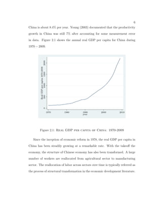
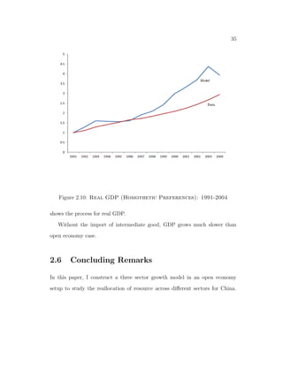
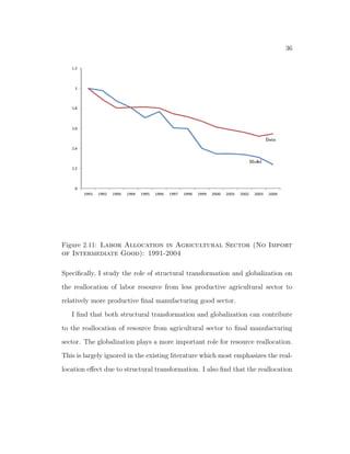
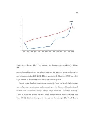
22. nal manufacturing goods to the rest of the world. This dissertation consists of three essays that attempt to shed light on how globalization impacts the economic growth in general and specially for the Chi- nese economy. Chapter 2 starts from the empirical facts of the China Miracle. I

23. rst review some empirical facts of the Chinese economy since China opens its economy to the world in 1978. I construct a neoclassical growth model to reconcile these facts. Recent growth literature emphasizes the misallocation of resource at the micro level could reduce TFP at the macro level. Both structural transformation and globalization in China contribute to correct the misallocation of resources in China. Hence they could account for the remarkable growth experience of China. In this essay, I develops a growth model that emphasizes the role of structural transformation and international trade to account for the growth experience of China. Structural transformation releases a large population living in agricultural sector and makes China have comparative advantage in labor intensive manufacturing production. The model is also built on the fact that

24. 3 the processing trade is pervasive in China. The import of intermediate goods also releases labor to more productive manufacturing good sector. I calibrate the model to match relative prices of agricultural good and intermediate good and show that the process of structural transformation in an open economy can generate growth rate of GDP comparable to those observed in China in the period 1991-2004. Chapter 3 studies how international trade impacts economic growth in general. In this essay, I build a theoretical model to study the eect of trade liberalization on the innovation in an economy. Build on Grossman and Help- man (1991), I combine a creative destruction model with an international trade model with heterogenous

25. rm a la Melitz (2003). I study the balanced growth path of this simple model. Then I examine the impact of trade on economic growth. Trade liberalization in terms of reduction of trade barrier can help reallocate labor to innovation sector and therefore will promote the economic growth of the economy. Chapter 4 reviews the literature on structural change and its implications for economic development. Developing countries started to develop from reallocating labor in agriculture to industrial production. This essay reviews the two main mechanism to generate structural change in standard models of economic growth. The structural change can arise from the nonhomothetic preference (or Engle's Law). Once the food problem is solved for poor countries, they can reallocate labor to manufacturing production. The other mechanism that can generate the structural change is from the dierent productivity growth across

26. 4 sectors. Then I review the application of the framework of structural change to study a variety of issues in developing countries. I also review the recent development of theoretical models of structural change both in closed economy setup and in an open economy setup.

27. Chapter 2 Reallocation, Globalization, and Economic Growth in China 2.1 Introduction China becomes the second largest economy in terms of GDP in the world as this paper is being written. This paper attempts to study the Chinese economy in a global perspective. We emphasize the role of structural transformation and international trade in the reallocation of labor from less productive agricultural sector to more productive

28. nal manufacturing sector. The reallocation of labor provides China a comparative advantage in labor intensive manufacturing production. China started economic reform in 1978. Since then, the growth experience of Chinese economy has been remarkable. During 1978-2003, the growth of GDP of 5

29. 6 China is about 8.4% per year. Young (2003) documented that the productivity growth in China was still 7% after accounting for some measurement error in data. Figure 2.1 shows the annual real GDP per capita for China during 1970 2009. Figure 2.1: Real GDP per capita of China: 1970-2009 Since the inception of economic reform in 1978, the real GDP per capita in China has been steadily growing at a remarkable rate. With the takeo the economy, the structure of Chinese economy has also been transformed. A large number of workers are reallocated from agricultural sector to manufacturing sector. The reallocation of labor across sectors over time is typically referred as the process of structural transformation in the economic development literature.

30. 7 The structural transformation in China provides a comparative advantage in low cost manufacturing for China. With a comparative advantage in the labor intensive industry, China becomes a

31. nal processing and assembly platform for a large quantity of imports from other Asian countries to developed countries through China. This paper studies the role of structural transformation and globalization in the process of economic development in China. The reallocation of labor from less productive agricultural sector to more productive manufacturing sector provides the necessary workers for producing manufacturing goods. A large number of workers from rural area keep the wage low enough to make Chinese exports competitive in the world market. Young (2003) indicates that labor reallocation from agricultural sector is important for China's fast growth during the period between 1978-1998. To better ac- cess to the world market, China opened its economy since the beginning of the economic reform. The world market provides both the market for selling

32. - nal manufacturing goods and the market for importing the intermediate goods. Jones (2011) shows that developing countries are less productive to produce intermediate goods. The import of intermediate good to assemble

33. nal manufacturing goods is important for economic development in China. Since China is less productive in producing sophisticated intermediate goods, the import of intermediate goods releases labor to more productive assembling

34. nal manufacturing goods. Both structural transformation and the international trade contribute to the reallocation of labor from less productive sectors to more productive sectors. Hence they improve the economic performance of China. This

35. 8 paper studies the role of structure transformation and international trade in the reallocation of labor and in turn the economic growth in China. In this paper, I show that both structural transformation and international trade can account for the labor reallocation from agricultural sector to

36. nal manufacturing sector in the data. In addition to the existing literature1, I

37. nd that international trade also plays a very important role in the reallocation of labor from agricultural sector to

38. nal manufacturing good sector. Without international trade, labor reallocation process becomes much slower and the decline of labor allocation in agricultural sector is only about 10%. The international trade in the model can account for more than 50% of decline of labor share in agricultural sector. In order to formalize the idea, I develop a three-sector neoclassical growth model with structural transformation in an open economy setup. There are three sectors: agricultural sector, intermediate manufacturing good sector, and

39. nal manufacturing good sector. In a recent paper Brant, Hsieh, and Zhu (2008), they identify that the central driving force behind structural transformation in China is the improvement in nonagricultural TFP relative to agricultural TFP. In the model, I consider two methods to generate the structural transformation. Following the standard literature on structural transformation, I use a non-homothetic preference with a subsistence consumption level for agricultural good as in Restuccia, Yang, and Zhu (2008). In the model, TFP also grows faster in manufacturing sector relative to agricultural sector. Fast growing manufacturing sector also drives people out of the agricultural sector. Another 1Most existing literature only emphasizes the process of structural transformation in the labor reallocation process and do not consider the role of international trade.

40. 9 driving force behind labor reallocation in China is the import of intermediate goods. With large exports, China employs a variety of inputs from foreign countries. Koopman, Wang, and Wei (2008) develops a general formula to estimate that the share of foreign content of China's exports is at about 50%: For some sectors that are relatively sophisticated such as electronic devices, the share is particularly high and about 70%: In the model, I introduce intermediate good in the production function a la Jones (2011). The share of intermediate good will amplify the eect of productivity growth of manufacturing sector on the labor allocation in equilibrium. The model in this paper is build in an open economy setup. Even though China exports a lot of manufacturing goods, China does not have a big bargaining power to set the price in the world market. Hence all prices of traded goods in the model are given at the level of international prices. In equilibrium, the international prices levels also aect the labor allocation. Under the international trade, domestic market can also import agricultural good if the domestic price is above the international price. China has to support a large population. To satisfy the subsistence consumption of agricultural good, China has to devote a large fraction of labor into the production of food before China opened its economy to the world market. By importing agricultural good, it can also release the labor to other sectors. Allowing import of agricultural good accelerates the process of structural transformation in China. The model is calibrated to the data of China to account for the growth experience in China. I

41. nd that the model can replicate the labor reallocation

42. 10 process in data of China during the period 1991-2004. With international trade, the model predicts a much faster annual growth rate of real GDP than the data shows. In a closed economy, the model fails to account for the growth experience during the period. The model only predicts a 2:4% annual growth rate of real GDP. This highlights the importance of international trade for the process of economic growth in China. Finally, I relax the subsistence consumption requirement and

43. nd that the model can still account for the growth experience though the model predicts a larger decline of labor share in agricultural sector. The model with homothetic preferences predicts an annual growth rate 11% of real GDP. 2.1.1 Related Literature First, this paper is related with the literature on structural transformation. The theoretical models on structural transformation lie in two lines of research. The

44. rst line is based on Kongsamut, Rebelo, and Xie (2001) and emphasizes a role in non-homothetic preferences consistent with Engel's law. The second set of models are based on Baumol (1967) which emphasizes structural change is a result of dierential productivity across dierent sectors. A more recent paper along this line is Ngai and Pissarides (2007). The structural transformation in their model is a result of sector-biased productivity growth and the elasticity of substitution between sectors is less than one. All of these models deal with structural transformation in a closed economy. Second, this paper extends the models of structural transformation to an

45. 11 open economy setup among other papers. Matsuyama (1992) and Matsuyama (2009)

46. rst start the discussion of structural transformation in an open economy context. Matsuyama (1992) is close to this paper in the spirit. We both emphasize the role of agricultural sector for structural transformation and study the implication for economic growth. A recent paper Yi and Zhang (2011) intro- duces Ricardian type international trade model as Eaton and Kortum (2002) into Ngai and Pissarides (2007) to study the structural transformation in an open economy. Another paper Teignier-Baqu (2009) extends a neoclassical growth model into an open economy setup and employs a non-homothetic preference to study the role of international trade in structural transformation. He also calibrates the model to the data of U.K., U.S., and South Korea to explore the quantitative implications of international trade on structural transformation. He

47. nds that the import of agricultural good can accelerate the process of structural transformation. Thirdly, this paper is related to the research on the transition of Chinese economy. This paper follows Brant and Zhu (2010) and Dekle and Vanden- broucke (2006) to account for growth and structural transformation for Chinese economy. However, these two papers only do the quantitative analysis in a closed economy setup. The contribution of this paper is to extend the analysis to an open economy setup by emphasizing the import of intermediate goods as well. My paper also relates to the literature that studies the role of agricultural sector for economic development. Restuccia, Yang, and Zhu (2008)2 2Other papers discuss the role of agricultural sector including Gollin, Parente, and Roger- son (2007) and Hayashi and Prescott (2008). Gollin, Parente, and Rogerson (2007) studies

48. 12 emphasizes the food requirement for a country's economic development. With a low productivity level in agricultural sector and subsistence food requirement, developing countries need to put a large number of people working in the agricultural sector to satisfy the food requirement. In an open economy setup, the import of agricultural goods can relax the food requirement problem for China and accelerates the process of structural transformation. Finally, this paper is related to the literature on resource reallocation on aggregate TFP for China3. A recent paper on this issue is Hsieh and Klenow (2009). They use establishments level data and

49. nd that TFP can gain 30%- 50% in China after reallocation of capital and labor to equalize the marginal products to the extent observed in the U.S. Another important paper on reallocation within manufacturing sector of Chinese economy is Song, Storesletten, and Zilibotti (2011). They identify that reallocation of labor and capital across manufacturing

50. rms has been a key source of productivity growth. Bajona and Chu (2010)

51. nd that the reallocation of resource from state owned sector to non-state owned sector due to the cut of government subsidy required by WTO can provide welfare gains. Along this line of research, I study the reallocation across dierent sectors and

52. nd that reallocation of labor across sectors in China can also improve the growth. The rest of this chapter is organized as follows. Section 2 documents some the dierent economic performance in agricultural sector for countries can account for the dierent income levels. Hayashi and Prescott (2008) makes the point that the impediment of reallocation from agricultural sector to more productive sector will slow down the economic growth. They show the case for Japanese economy in the prewar period. 3Kehoe and Ruhl (2009) studies the resource reallocation between nontraded sector and traded sector of Mexico to account for the output drop after crisis.

53. 13 empirical facts about the transformation of Chinese economy. Section 3 de- scribes the economic environment. Section 4 discusses the calibration of the model to the data of Chinese economy. Section 5 reports and discusses the results. Section 6 concludes. 2.2 Empirical Evidence: The China Miracle In this section, we document some of the main empirical facts of China's economic transformation. Figure 2.1 has shown the remarkable growth experience of China since the inception of economic reform. In this section, we mainly document the empirical facts on structural transformation in China. Since the beginning of economic reform in 1978, the rural population has been declined signi

54. cantly. Figure 2.2 shows the data on rural population as a percentage of total population from the World Bank. The percentage of rural population has declined from more than 80% to slightly above 50%: During the same period, the value added of agricultural sector has also been decreased sharply. The value added of agricultural sector decreases from about 40% to 20% of the aggregate economy. The reallocation of the labor resource to manufacturing sector provides the productive capacity for large exports to the world market. One of the main policy of economic reform in China is to open its economy to the world market. Starting from the reform, the international trade as percentage of GDP increases sharply. In December 2001, China entered the WTO

55. 14 Figure 2.2: Rural Population as a percentage of Total Population of China: 1970-2009 and international trade has increased dramatically since the accession to the WTO. Figure 2.4 shows the data of merchandize trade as a percentage of GDP. On the one hand, China exports a large amount of manufacturing goods to the world market. On the other hand, China imports a lot of raw material and intermediate goods as inputs to produce the manufacturing goods. The processing trade is pervasive in China.

56. 15 Figure 2.3: Value Added as a percentage of GDP in Agriculture (Source: World Bank World Development Indicators) 2.3 The Model The model is built on models of structural transformation and features both dierential productivity growth and non-homothetic preferences. Final manufacturing sector is more productive than agricultural sector and also grows faster than agricultural sector and intermediate good sector. This provides the comparative advantage of manufacturing production and hence the incentive for international trade. In the model, there are three sectors: agricultural sector, intermediate manufacturing good sector and

57. nal manufacturing sector. The

58. 16 Figure 2.4: International Trade as a percentage of GDP (Source: World Bank World Development Indicators) non-homothetic preference imposes a subsistence requirement for household. 2.3.1 Household The representative household consumes both agricultural good and

59. nal manufacturing good. Also there is a subsistent level requirement of consumption of agricultural good. The income of household comes from the wage income from selling labor to

60. rms, the rent income from land and rent income from capital.

61. 17 The preference of the household is as follows u (cat; cmt) = b log (cat a) + (1 b) log (cmt) : (2.1) where ca is the consumption of agricultural good, a is the subsistence level of agricultural good, and cm is the consumption of manufacturing good. b is a parameter. The representative household will maximize the life-long discounted utility given by X1 t=0

62. tu (cat; cmt) (2.2) where u (cat; cmt) is de

63. ned above. The representative household will sell labor to dierent sectors: agricultural sector, intermediate good sector, and

64. nal manufacturing good sector. The total income will be used for consumption and investment. The budget constraint for the representative household is given by pmt+1It = wtL + pmtrtkt + tH pmtcmt patcat (2.3) kt+1 = (1 ) kt + It (2.4) k0 is given. where It is the investment, L is the total labor endowment, kt is capital, H is land in

65. xed supply and wt is the wage rate for working in dierent sectors, rt is the rental rate on capital, t is the rental rate on land, pmt; pat are prices on

66. 18

67. nal manufacturing good and agricultural good respectively. The representative household's problem is to maximize the life-long utility (2.2) subjective to budget constraints (2.3) and (2.4). 2.3.2 Technologies There are three sectors in the model. Each sector has its own technology. The technology for agricultural good sector is given by Yat = Aatl atH1 : (2.5) where Yat is the output of agricultural good sector, At is the productivity of the sector, lat is the labor allocation of the sector, H is the land endowment in

68. xed supply. is the parameter of labor income share of agricultural sector and is between zero and one. Agricultural good is produced by labor and land. The technology for

69. nal manufacturing good sector is given by Ymt = Amt k mtl1 mt 1 X t : (2.6) where Ymt is the output of

70. nal manufacturing good sector, Amt is the productivity of the sector, kmt is the capital used in the sector, lmt is the labor allocation in this sector, Xt is the intermediate good used in the production of

71. nal manufacturing good. and are parameters of income share of capital and intermediate goods. Both parameters and is assumed between 0 and 1:

72. 19 The technology for intermediate manufacturing good sector is given by Yit = Aitlit (2.7) where Yit is the output of intermediate good sector, Ait is the productivity, and lit is the labor allocation to intermediate good sector. We assume that intermediate good is only produced by labor. Later, we will focus on the case that intermediate good will be imported from foreign countries since the domestic country is not productive at producing the intermediate good. This is also consistent with the fact that China has imported a large share of intermediate good as I mentioned in the Introduction. The

73. rms' problems are to maximize their pro

74. ts given the prices. Final Manufacturing good producer's problem: Taking the prices of pmt; pit and factors returns on labor and capital as given, the representative

75. rm in the

76. nal manufacturing good sector is to maximize max pmtAmt k mtl1 mt 1 X t wtlmt rtkmt pitXit (2.8) Similarly, taking the prices of pat and factors return on labor wt and land t as given, the representative

77. rm in agricultural sector solves the following problem max patAatl atH1 wtlat tH: (2.9) And taking the price pit and wage of labor wt as given, the representative

78. rm

79. 20 in intermediate good sector solves the following problem max pitAitlit witlit: (2.10) 2.3.3 Equilibrium First, I consider an open economy setup. Here I study a special case of equilibrium. In this equilibrium, the domestic country has a comparative advantage in producing

80. nal manufacturing good and the rest of world has a comparative advantage in producing intermediate good. Hence the pattern of trade is that China imports intermediate manufacturing good and export

81. nal manufacturing good. The trade pattern here I consider is consistent with the actual trade pattern for China. Even though China imports and exports a lot of manufacturing goods in the world market, China still does not have much bargaining power in the world market. Hence I assume that China takes all international prices of traded goods as given by the world market. We study an equilibrium of this small open economy. The de

82. nition of an equilibrium of the economy is given as follows. De

83. nition 1 Given initial resources endowments fk0; L;Hg and international prices p at; p it; p mt in the world market, also given the sequences of factor rental prices fwt; rt; tg; a competitive equilibrium is a sequence of household consumption plans fcat; cmtg and production plans of

84. rms fyat; ymt; yit; kt; lat; lit; lmtg such that The representative household chooses the consumption plans fcat; cmtg

85. 21 and kt to solve utility maximization problems. Firms choose production plans to solve pro

86. t maximization problems and earns zero pro

87. t in equilibrium. All markets clear. { commodity market clearing conditions: ymt = cmt + It + xmt; (2.11) yat = cat mat; (2.12) Xt = mit: (2.13) where xmt is the export of

88. nal manufacturing goods, mat is the import of agricultural good, and mit is the import of intermediate manufacturing good. { Labor market clearing condition lat + lmt = L: (2.14) where L is the total labor endowment. Trade is in zero balance.4 p mtxmt = p itmit + p atmat: (2.15) 4Since the trade balance of China does not change very much over time, to add a surplus term in the model will not change the result.

89. 22 And the no-arbitrage condition between the capital and land assets holds. 2.3.4 Characterization The analysis of the model starts from the household problem. All the derivations are gathered in the appendix. The solutions to household problem give us the consumption plan. cat = b (wtL + tH + rtkt) + (1 b) pata pat ; (2.16) cmt = (1 b) (wtL + tH + rtkt pata) pmt : (2.17) From above two equations, we can know that the requirement of subsistent level of consumption a is important for allocation of consumption. If the value of a is very high, then the consumption of agricultural good is also high. It will need more resource to allocate to agricultural sector and impede the development. The solutions to

90. rms problems give us the labor allocation in dierent sectors given prices. The FOCs for

91. rm's problem in agricultural sector are given by wt = patAatl 1 at H1 ; (2.18) t = (1 ) patAatl atH : (2.19)

92. 23 These two equations also give us the wage and rental rate on land in the agricultural sector. Combining these two equations, we can obtain a equation for labor allocation in agricultural sector. lat = 1 1 1 t patAat 1 H (2.20) From the above equation, we can know that labor allocation in agricultural sector depends on the rent on land, price of agricultural sector and productivity of agricultural good. In addition, from eqs. (2.18) and (2.19) we can obtain 1 H lat = wt t : (2.21) We will use this equation to calibrate the share of labor in agricultural sector. Solving

93. rm's problem in

94. nal manufacturing good sector gives us the following FOCs (1 ) (1 ) pmtAmt k t l1 mt X t k t l mt = wt; (2.22) (1 ) pmtAmt k t l1 mt X t k1 t l1 mt = rt; (2.23) pmtAmt k t l1 mt 1 X1 t = pit (2.24) From eqs. (2.22) to (2.24), we can obtain several ratios of resource allocation which will be used to calibrate the parameters in the next section. From eq. (2.22) and eq. (2.23), we can obtain the ratio of labor allocation and capital

95. 24 used in the

96. nal manufacturing sector that depends on the factor returns. 1 kt lmt = wt rt (2.25) The demand for intermediate good is given by Xt k t l1 mt = pit pmtAmt 1 1 : (2.26) In equilibrium, the return on land and capital must be equal in the absence of arbitrage opportunity. This implies that 1 kt lmt = 1 H lat (2.27) From the FOCs for three dierent

97. rms and also the market clearing conditions for labor market, we can obtain the expression for labor allocation in agricultural sector. The result is summarized in the following proposition. Proposition 2 The labor allocation in the agricultural sector is given by (lat)1 = Aat A1=(1) mt ! pat pmt pit pmt 1 (2.28) where is parameter which depends on ; ; : Proof. See the Appendix. From eq. (2.28), we can see that the labor allocation of agricultural sector

98. 25 depends on the relative productivity of agricultural sector to

99. nal manufacturing good sector. If the growth of productivity in

100. nal manufacturing good sector outweighs the growth of productivity in agricultural sector, then the labor allocation is reallocated to the more productive

101. nal manufacturing good sector. This is the reallocation eect driven by the dierential productivity5. Notice also the labor allocation in agricultural sector depends on the relative price of agricultural good to

102. nal manufacturing good. A reduction of relative agricultural good will reduce the allocation of labor to agricultural sector. If the country opens to international trade and import the agricultural good, this will reduce the relative price of agricultural good. Labor will also be reallocated to the other sector. This is the reallocation eect due to international trade. Similarly, the reallocation eect can also happen if I allow the import of intermediate manufacturing good. We can also notice that the role of intermediate good share : Here is similar to a multiplier on the productivity of

103. nal manufacturing good sector. This is dierent from a standard model without intermediate good6. Given the speci

104. c value of as shown in the data for China7, the term 1 can also serve as a multiplier to amplify the eect of reduction in the price of intermediate good. Hence the labor reallocation eect is ampli

105. ed by including intermediate good since all the production activities are correlated through intermediate goods. 5This is the machanism that emphasizes in the papers Baumol (1967) and Ngai and Pis- sarides (2007) 6However, this is similar to Jones (2011). In his paper, the intermediate good share also has a role of multiplier. 7In the data, is 0:64 for China as suggested by Jones (2011).

106. 26 In the next section, we use data of China to calibrate the model based on the eq. (2.28). 2.4 Calibration In this section, I calibrate the model in the previous section to match the data of China. I use the FOCs derived in the previous section to calibrate the parameters of capital share and labor share to match the data in input-output table of China: The calibrated values of parameters are reported in Table 2.1 as follows. Table 2.1: Calibration of Parameters Parameter Value Target Capital share in manufacturing sector 0:41 capital share in I/O Labor share in agricultural sector 0:52 labor share in I/O Intermediate good share 0:60 I/O table To calibrate the model to the data, we need to specify the productivity growth process. I assume that

107. nal manufacturing sector is more productive than agricultural sector in the initial period. Following the literature on estimation of productivity of China, I assume that productivity grows at 3% per year for

108. nal manufacturing sector and no growth in agricultural sector for nor- malization. Hence this assumption has already take the productivity growth in agricultural sector into consideration. Since in the model, the labor allocation only depends on the relative productivity of agricultural sector to

109. nal manufacturing sector, I can normalize the productivity growth of agricultural sector

110. 27 to be zero. To construct the series of international prices, I use unit value to approximate the international prices. It is usually dicult to obtain price data in international trade. Usually, unit value is used to approximate the price data. I obtain data of quantity and value of international trade data between China and the U.S. from OECD SITC (rev. 2). I obtain the quantity and value data and calculate the unit value. For agricultural price, I use the unit value data of wheat to approximate the price of agricultural good. I choose the data between China and U.S.. For agricultural good, I use the data on quantity and value of export of wheat from U.S. to China. This data is available from OECD. I choose textile commodity as the

111. nal manufacturing good since China exports a lot of this kind of commodity to the world market. The intermediate good that I choose is the cotton fabrics to produce the textile product. I use the quantity and value data of import of cotton fabrics from U.S. to China to calculate the international price of intermediate good. Also for

112. nal manufacturing good textile product, I use the quantity and value of export from China to U.S. to calculate the unit value as an approximation of the international price of

113. nal manufacturing price. The problem with this method is that it will bring a large uctuation of the results when we simulate the model. After the calibration of the model, I simulate the model for the period from 1991 to 2004 due to restriction of data availability of quantity of trade between China and U.S.. The results are discussed in the next section.

114. 28 2.5 Results In this section, I report and discuss the results for dierent cases. Speci

115. cally, I consider three dierent cases of the model. First, I simulate the model in the open economy setup for the period 1991 2004. Then I consider an experiment to switch o all international trade and to compare with the case of an open economy. Finally, I consider the homothetic preferences case in which the preferences are no longer subject to a subsistence consumption requirement. A preview of the results is shown in Table 2.2 as follows. Table 2.2: Results Baseline Closed Homothetic No Import of Data Model Economy Preferences Intermediate Labor Allocation 40% 42% 10% 79% 70% Growth of GDP 8:6% 13:5% 1:7% 11:1% 5:7% In the open economy, I assume that domestic country is a price taker and therefore all international prices are taken as given. In the last section, I have discussed the way I construct the series of international prices for agricultural good, intermediate good, and

116. nal manufacturing good. I simulate the model for the period 1991-2004. The result is given by Fig- ure 2.5 for allocation of labor in the agricultural sector. Basically, the model of open economy version we consider in Section 3 can replicate the data for the period 1991-2004. We observe that there are some uctuations in the model since the international prices uctuate. In the data during 1991-2004, the labor has been

117. 29 Figure 2.5: Labor Allocation in Agricultural Sector (open economy setup): 1991-2004 declined by 40% and the model predicts that labor in the agricultural sector is declined by 42%. The real GDP in the model is calculated as GDP = pa0Yat + pm0Ymt pi0Xt where pa0; pm0; pi0 are prices measured in the base period. The simulation results are given by Figure 2.6.

118. 30 Figure 2.6: Real GDP (open economy setup): 1991-2004 Basically, the model replicates the data. However, GDP in the model grows much faster than GDP in the data after 2001. In the data, the average growth rate of real GDP during 1991-2004 was about 8:6%: However, the model predicts an annual growth rate of more than 10%: This could be driven by the uctuations of international prices in the data. The result in this case depends heavily on the international prices. One possible explanation of the much higher growth of real GDP in the model is China's accession to WTO and the output of

119. nal manufacturing good increases due to the large demand from the rest of

120. 31 world. To make comparison and examine the role of reallocation, I then consider a closed economy version of the model. The dierence between open economy version and closed economy version are the endogenous prices. In closed economy, prices of all three goods are determined by the market clearing conditions. Since we switch o the international trade, we can expect that the prices of agricultural good and intermediate good must increase. From the Proposition 2, we know that this will impede the reallocation of labor from agricultural sector to

121. nal manufacturing sector. The results are given by Figure 2.7. From Figure 2.7, we can see that the reallocation is not clearly shown and is about 10% which is far lower than the data shows. The slightly decrease of labor allocation in agricultural is driven by the productivity growth. Comparing Figure 2.7 and Figure 2.5, we can see that international trade has played a very important role in the reallocation process. The globalization can account for more than 50% of the reallocation of labor from agricultural sector to the

122. nal manufacturing sector as suggested by the model. The similar conclusion can be drawn for real GDP as shown in Figure 2.8. Without the international trade, the growth of real GDP slows down. How- ever, the productivity growth still contributes to the growth of the economy. Also from the comparison between Figure 2.6 and Figure 2.8, we can notice that the important role of reallocation of resource in the process of economic development. The impediment of resources reallocation makes the economy grow slower.

123. 32 Figure 2.7: Labor Allocation in Agricultural Sector (closed economy setup): 1991-2004 In another numerical example, I relax the subsistence consumption requirement i.e., set a = 0: In this case, I also consider the the implications of the model for labor reallocation and real GDP. The reallocation of labor is shown in Figure 2.9. The model predicts a larger share of labor has been reallocated away from agricultural sector as opposed to the data. In the case of homothetic preference, the relax of subsistence consumption requirement accelerate the reallocation process of labor to faster growing manufacturing sector. We no longer need to

124. 33 Figure 2.8: Real GDP (closed economy): 1991-2004 allocate a

125. xed amount of labor to produce the subsistence level of agricultural good. The result of real GDP is shown in Figure 2.10. The model implies a faster growth rate of real GDP during the period than the case of closed economy. This shows that the importance of a subsistence consumption requirement. The subsistence consumption requirement of agricultural good can be a big obstacle for the development of an economy. This is consistent with the

126. ndings of Gollin, Parente, and Rogerson (2007).

127. 34 Figure 2.9: Labor Allocation in Agricultural Sector (Homothetic Preferences): 1991-2004 In this experiment, I consider a situation with no import of intermediate good. However, I still allow the international trade of agricultural good. Hence the reallocation process can also be accelerated by importing the agricultural good. The growth of GDP will be impeded by allocating labor to less productive sector. The reallocation process is reported in Figure 2.11. The model can replicate the reallocation process of labor comparable with the data implies. The GDP grows slower than what the data shows. This experiment highlights the importance of import of intermediate good. Figure 2.12

128. 35 Figure 2.10: Real GDP (Homothetic Preferences): 1991-2004 shows the process for real GDP. Without the import of intermediate good, GDP grows much slower than open economy case. 2.6 Concluding Remarks In this paper, I construct a three sector growth model in an open economy setup to study the reallocation of resource across dierent sectors for China.

129. 36 Figure 2.11: Labor Allocation in Agricultural Sector (No Import of Intermediate Good): 1991-2004 Speci

130. cally, I study the role of structural transformation and globalization on the reallocation of labor resource from less productive agricultural sector to relatively more productive

131. nal manufacturing good sector. I

132. nd that both structural transformation and globalization can contribute to the reallocation of resource from agricultural sector to

133. nal manufacturing sector. The globalization plays a more important role for resource reallocation. This is largely ignored in the existing literature which most emphasizes the reallocation eect due to structural transformation. I also

134. nd that the reallocation

135. 37 Figure 2.12: Real GDP (No Import of Intermediate Good): 1991- 2004 arising from globalization has a large eect on the economic growth of the Chi- nese economy during 1991-2004. This is also suggested in Jones (2010) as a hot topic studied in the current literature of economic growth. In this paper, I only consider the economy of China and studied the importance of resource reallocation and economic growth. However, liberalization of international trade cannot always bring a bright future for a country's economy. There is no simple relation between trade and growth as shown in Kehoe and Ruhl (2010). Similar development strategy has been adopted by South Korea

136. 38 during 1960s and it did contribute to the growth miracle of South Korea as shown in Connolly and Yi (2009). However, the similar development strategy does not work in Mexico as documented by Kehoe and Ruhl (2010). Hence there must be some missing factors that can also link international trade and economic growth for a country and they will be left for future exploration.

137. Chapter 3 When Schumpeter meets Melitz: An Endogenous Growth Model with Heterogeneous Firms 3.1 Introduction Recent empirical evidence shows that the heterogeneity among dierent

138. rms is crucial for understanding the within industry trade. Since Melitz (2003), trade literature has introduced

139. rm level heterogeneity into international trade models to account for the new empirical facts at the

140. rm level. Firm level empirical evidence shows that there are large and persistent productivity dierences across

141. rms. However, these

142. ndings have not been re ected in the literature of endogenous economic growth. 39

143. 40 Pioneered by Romer (1986) and Romer (1990), endogenous growth literature focuses on the introduction of new goods. They assume that every

144. rm has the same productivity level and those endogenous growth models are studied in a closed economy. Hence, when we study these models in open economy, all the

145. rms will export. However, this is not consistent with the

146. rm level empirical evidence of trade. Firm level empirical evidence shows that not all the

147. rms will export even in the traded goods sector. To consider the economic growth in an open economy, we need to take

148. rm heterogeneity into consideration by assuming that

149. rms have dierent productivity levels. There is a large literature on the impact of international trade on economic growth. A recent paper Lucas (2009) shows that openness can contribute to the economic growth. Lucas (2009) emphasizes the importance of ow of ideas among dierent countries especially ow to the underdeveloped countries. He argues that it is the ow of idea that is the main force to reduce the income inequality and for the convergence of growth to a common growing level. Lucas (2009) uses a simple mechanical model to describe the ow of ideas. The key parameter of the model is calibrated from the open economies which is based on Sachs and Warner's classi

150. cation Sachs and Warner (1995). He

151. nds that income levels and growth rates converge in open economies. However, Lucas (2009) has no explicit role of international trade and the only evidence on trade comes from the calibration of the key parameter using data from those open economies based on Sachs and Warner classi

152. cation Sachs and Warner (1995). Hence we need a theory to explain why economic interactions can promote

153. 41 growth. Lucas (2009) uses Sachs and Warner's classi

154. cation which is subject to crit- icize. Rodriguez and Rodrik (2000) provides a critical survey on the literature of the impact of trade and growth. They argue that the

155. ndings on trade and growth are less robust than claimed. Moreover, the recent cross-sectional research con

156. rm the criticisms of the Sachs-Warner

157. ndings by showing that the results are sensitive to the openness classi

158. cation used in 1970-89 and do not hold for the 1990s. Another recent paper Wacziarg and Welch (2008) update the Sachs-Warner classi

159. cation and results. They also address the critique of Rodriguez and Rodrik (2000). Hence we need to look at a more broad literature on the empirical

160. ndings of trade's impact on growth. Before we build the model to study how trade can promote growth, we need to scrutinize some empirical

161. ndings about trade's impact on growth. There is a large empirical literature on the relationship between trade and growth. Here I will not exploit all the literature and I will only choose some important ones to establish the empirical fact that trade could promote growth. Frankel and Romer (1999) provides an empirical investigation of the impact of international trade on standards of living. In the empirical literature which study trade's impact on income, one diculty of the OLS estimation is that the trade share may be endogenous. Hence the OLS estimation is not ecient and we need to control the problem of endogeneity. Frankel and Romer (1999) constructs measures of geographic component of countries' trade as instruments. They

162. nd no evidence that Ordinary least-squares estimates overstate the eects of trade

163. 42 on growth. Further, they

164. nd that trade has a quantitatively large and robust positive eect on income. Wacziarg and Welch (2008) also studies the eect of trade liberalization on growth. They provide some new evidence by updating Sachs-Warner's classi

165. cation. Using new data set over 1950-98 period, countries that liberalized their trade regimes experienced average annual growth rate that were about 1.5 percentage point higher than before liberalization. Related Literature Eaton and Kortum (2001) develops a theoretical structure that uni

166. es innovation, international trade and economic growth. We will follow this strand of research to consider trade and growth based on innovation. Baldwin and Robert-Nicoud (2008) explores the impact of trade on growth when

167. rms are heterogeneous in productivity. They

168. nd that greater openness produces both anti- and pro-growth eect. They tried dierent endogenous growth models based on the variety expansion including Grossman-Helpman, the Coe- Helpman, and the Rivera-Batiz-Romer Model. A closely related paper is Unel (2010) which considers the technology diusion and trade. He integrates Melitz (2003) on trade and heterogeneous

169. rms into the product innovation endogenous growth model developed by Romer (1990). He

170. nds that exposure to trade can increase average productivity. However, the positive eects may not be high enough to cover the cost. Then his model like Baldwin and Robert- Nicoud (2008) produces an ambiguous result on trade and growth. Atkeson and Burstein (2010) develops a general equilibrium model of the decisions of

171. rms to innovate and to engage trade. They

172. nd lower trade cost has a substantial

173. 43 eect on

174. rms' decision of entry, exit, trade and innovation. However, they fail to

175. nd that reduction of trade cost has a substantial impact on aggregate productivity. Haruyama and Zhao (2008) also studies the eect of trade liberalization on the aggregate productivity and the growth of productivity in an RD based model with heterogeneous marginal cost for

176. rms. Speci

177. cally, they use a quality-ladder model of growth to model the RD process. They argue that trade liberalization can increase the rate of technical progress as well as the level of manufacturing productivity. We follow this paper to build our model by combining a creative destruction growth model developed by Aghion and Howitt (1992) and Melitz (2003). As in Haruyama and Zhao (2008), each innovation in my model is an improvement of the quality of the good. The engine of growth in my model is the continual improvement of quality of good. We use Aghion and Howitt (1992) and Grossman and Helpman (1991) to include creative destruction into the innovation process. That is, the prospect of more future research discourages current research since more future research reduces the rent accrued by current monopolist. The

178. - nal product is produced using intermediate goods. Each intermediate good is produced by a monopolist. Firms which produce intermediate goods are heterogeneous in productivity level. Each

179. rm who wants to enter the market has to make innovation to improve the quality of current goods. Firms pay

180. xed cost to make innovations and enter the market by replacing the incumbent. Then

181. rms can pay a

182. xed cost to export to sell in the foreign market. Here I use Melitz (2003) to formalize the idea of international trade with heterogeneous

183. 44

184. rms. Then each intermediate good is associated with one productivity level as in Melitz (2003). I derive the balanced growth path of the economy and study how trade liberalization impacts the growth. We

185. nd that trade liberalization can aect the cuto value of productivity for

186. rms to make innovation and export. That is, trade liberalization can help reallocate the labor to export behaviors of

187. rms. Trade liberalization refers to the reduction of iceberg transportation cost and the reduction of sunk cost for export. We

188. nd that trade liberalization can make

189. rms more likely to export. However, it also makes

190. rms more dicult to make innovation and enter the domestic market. In this sense, trade liberalization drives the least productive

191. rms out of the market. Hence it increases the average productivity of the economy. Trade liberalization can also help reallocate labor to do RD. The engine of growth is the improvement of quality through doing RD by

192. rms. Hence the reallocation of labor to do RD consequently increase the growth of the economy. We

193. nd that trade can indeed promote the growth of the economy. The remaining of the paper is organized as follows. Section 2 presents the set up of the model. Section 3 analyzes the steady state equilibrium and solve for the balanced growth path. Section 4 studies the impact of trade liberalization. Section 5 concludes. Some of the derivations are gathered in the Appendix.

194. 45 3.2 The Model We embed Melitz (2003) into a creative destruction model of endogenous growth Aghion and Howitt (1992) Speci

195. cally, we use Grossman and Helpman (1991) to model the innovation process. The engine of the growth for the economy is the improvement of the quality of goods. We use Erzo's formulation of quality ladders model as in Luttmer (2009). 3.2.1 Consumer Time is continuous. Consumers derive utility from aggregate consumption. The consumer's problem is formulated as follows max Z 1 0 et ln (Ct) dt (3.1) s:t: Z 1 0 exp Z t 0 rsds Ctdt wealth: (3.2) Solving this dynamic optimization problem leads to the usual

196. rst order condition for consumer _C t Ct = rt : (3.3) Ct is aggregate consumption which is a composite Ct = exp Z 1 0 ln (ct (!)) d! : (3.4) Each intermediate good comes in dierent vintages with dierent quality

197. 46 level. Let St (!) be the number of the latest vintages which have been introduced at time t: Then we have ct (!) = SXt(!) n=0 ncn;t (!) : (3.5) 3.2.2 Producers The

198. nal good is produced using intermediate goods. Each intermediate good is produced by a monopolist by replacing the incumbent. The production of intermediate goods only require labor. Each

199. rm produces an intermediate good. As in Melitz (2003), the production function for the owner of a blueprint for vintage n of commodity ! can use one units of labor to produce 'l units of the vintage. That is, n'l in terms of date 0 units of commodity !: Assume that each

200. rm has a dierent productivity level ' and each good is associated with one productivity level. Hence we can index the goods using productivity level ': All

201. rms engage Bertrand competition. The frontier producer faces the competition from the second-best quality producer. The unit pro

202. t for the frontier producer is xt (') = pt (') St(')' wt: (3.6) The second-best producer's pro

203. t is pt (') St(')1' wt: (3.7) The frontier producer could shut down the second-best producer by setting

204. 47 price pt (') as pt (') = wt St(')1' : (3.8) Then the unit pro

205. t of the frontier producer is xt (') = wt ( 1) : (3.9) From the product market equilibrium, we can obtain the ow pro

206. t for the producer is t (') = 1 1 Ct: (3.10) If the

207. rm exports to foreign countries, the ow pro

208. t from selling in the foreign market is xt (') = 1 Ct (3.11) where 1 is the iceberg transportation cost. 3.2.3 Innovations and Export Decisions To enter the market,

209. rms have to make innovation to improve the quality of the good. To make innovations,

210. rms have to incur sunk costs. Firms need to use some resources to do RD and the resources cannot be recovered. In this sense,

211. rms that do RD have to pay sunk costs. The RD cost for

212. rms to make innovation by improving the quality of good is f: Let v be the expected discounted value of ow pro

213. t in domestic market. If v f; then

214. rms will enter the domestic market by paying the sunk cost f and become a monopolist.

215. 48 Therefore we can determine a cuto value of productivity by v (') = f: (3.12) For

216. rms to export, they need to a

217. xed cost fx: Therefore

218. rms export if vx (') fx: Hence we can determine another cuto value of productivity by vx ('x) = fx: (3.13) 3.2.4 Creative Destruction and Value of Firms The idea of creative destruction was

219. rst proposed by Schumpeter (1942). In growth models, creative destruction is referred to the replacement of incumbent by new entrants to improve the quality or the technology. Aghion and Howitt (1992) and Grossman and Helpman (1991) are two earlier examples of creative destruction growth models. An entrant with a successful innovation can replace the incumbent in domestic market and earn the expected discounted value v of ow pro

220. t. The new entrant will receive the exact pro

221. t as the incumbent who is replaced by the entrant. Hence v (') has to follow the following equation rtvt (') = t (') + v_t (') mt (') vt (') : (3.14) Here mt is research eort exerted to improve the quality of good. This is the rate at which the incumbent will be replaced by a new entrant. This is also

222. 49 the term to measure the rate of creative destruction. For

223. rms who engage international trade with successful innovation, vxt can be obtained from serving the foreign market. Hence vxt will also follow a similar equation as follows rtvxt (') = xt (') + v_xt (') mt (') vxt (') : (3.15) vt (') and vxt (') measure the expected discounted value of ow pro

224. t. Re- call that

225. rms have to pay sunk cost for both of making innovation and exporting. Therefore, the net value of innovation for a

226. rm is given by Vt = Z 1 ' (v (') f) (') d' + Z 1 'x (vx (') fx) (') d': (3.16) where (') is the distribution of productivity levels over (0;1) : The

227. rst term in the above equation gives the net value of making innovation and the second term measures the net value of additional gain from serving the foreign market. 3.2.5 Labor Market There is no population growth in this model. The aggregate labor supply is Nt = N:1 Labor in this model has two purposes. One is to produce the

228. nal goods and the other purpose is to make innovation. Let Lt denote the labor devoted to produce the

229. nal good and Mt is used to make innovation. The labor 1However, we could include the population growth and this will not aect the result. See Haruyama and Zhao (2008), they consider a similar model with population growth to check the robustness of their model.

230. 50 market clearing condition is Lt +Mt = N: (3.17) Here we assume that the research eort is the same among all the industries. Therefore mt (') = Mt across all the industries. 3.3 Steady State Equilibrium In this section, we analyze a steady state equilibrium for the model. First we derive the following conditions about the determination of cuto values for productivity. The cuto value for

231. rms to enter the market f is given by f = 1 + Mt 1 1 Ct (') : (3.18) This equation is derived from eq. (9) ; (13) : Similarly, we can derive an equation for the cuto value of productivity for

232. rms to export. The equation for fx is given by fx = 1 + Mt 1 Ct (') : (3.19) These two equations help determine the cuto values of productivity for

233. rms to make innovation and export. The RHS of eq. (17) is the expected discounted ow pro

234. t of

235. rms at the cuto value of productivity '. Therefore (17) can give us the cuto value ': Similarly, eq. (18) give us the cuto value of productivity 'x for

236. rms to export. Remember, the aggregate consumption Ct which appears on the RHS of (17)

237. 51 and (18) depends on the productivity level ': Ct can be derived as Ct = exp Z 1 0 ln St(!) d! ' N + : (3.20) Substitute (19) into (17) and (18). Then we can determine the cuto values. Then we consider the RD decisions for

238. rms. The second equilibrium condition is about the RD decision. The expected value for

239. rms to make innovation is given by Z 1 ' 1 1 Ct (') d' + Z 1 'x 1 Ct (') 1 (') d': (3.21) The

240. rst term in the above equation is the expected ow pro

241. t from making innovation to enter the domestic market. The second term in the above equation measures the expected ow pro

242. t from export conditional on making innovation to enter the market by replacing the incumbent. The term (') = (1 (')) measures the conditional probability for a

243. rm that has already entered the market by making innovation. Hence equation (20) gives the expected payo from doing RD and make pro

244. t from serving both of domestic and foreign markets. Recall that

245. rms have to pay sunk costs to make innovation and export to sell in the foreign market. Therefore the expected sunk cost for

246. rms to enter both of the domestic and foreign markets is given by f + fx (') 1 (') : (3.22)

247. 52 Still, here we need to consider the conditional probability of

248. rms to export after making innovation to sell in the domestic market. To obtain an equilibrium, the expected ow pro

249. t from making innovations and export must be equal to the expected sunk costs of making innovation and export. The two terms on the RHS represent the expected cost from making innovation and export. Hence we obtain the following equilibrium condition Z 1 ' 1 1 Ct (') d' + Z 1 'x 1 Ct (') 1 (') d' = f + fx (') 1 (') : (3.23) The last equilibrium condition comes from the labor market clearing condition which we have discussed in the last section. This equilibrium condition is given by equation (16) : Now we can determine a balanced growth path of the model. Remember the engine of growth in this model is the continual improvements of quality for goods. Given the structure of the aggregate consumption as in equation (19) ; we can determine the balanced growth rate of the economy based on the arrival of improvement of quality. Following Luttmer (2009), we assume that the number of vintages follows a Poisson distribution with the density as given by ft (s) = (t)s et s! : (3.24)

250. 53 Also we assume Law of Large Number holds. Then we can obtain that Z 1 0 ln St(!) d! = ln () Z 1 0 St (!) d! = ln X1 s=0 sft (s) = ln () t: (3.25) Hence the growth rate of economy is ln () and is the arrival rate of improvement of quality. In this model, is Mt: The growth rate of the economy depends on the RD eorts measured by the workers allocated to RD sector. We summarize the result in the following proposition. Proposition 3 The growth rate of the economy is given by Mt ln (). 3.4 The Impact of Trade In this section, we study how trade liberalization can aect the growth of the economy. We try to explore the implications for growth models with creative destruction features in open economy. First, we consider the eect of trade liberalization on the cuto values of productivity. From eqs. (17) and (18) ; we can obtain the following relationship between two cuto values ' and 'x ' f = 1 'x fx : (3.26) Trade liberalization refers to the reduction of sunk cost for export and the reduction of iceberg transportation cost. We

251. rst consider the eect of reduction of sunk cost for export i.e., fx on the threshold of productivity value 'x: Ceteris

252. 54 Paribus, a reduction of sunk cost for exporting fx reduces the cuto value of productivity for

253. rms to export i.e., 'x decreases. This make

254. rms be easier to become exporters and also reallocate the resources from non-exporting sectors to exporting sectors. This is consistent with the standard literature as Melitz (2003). On the other hand, we will consider the eect of trade liberalization on the cuto value for

255. rms to make innovation and enter the domestic market. Also from equation (25) ; we

256. x the value of fx and hence the value of 'x: A reduction of iceberg transportation cost will increase the value of RHS of equation (25) : Hence ' has to increase. The increase of cuto value of productivity ' will make

257. rms more dicult to make innovation. In turn, this makes

258. rms be more dicult to enter the domestic market. Therefore, the less productive

259. rms will be driven out of the market and replaced by more productive

260. rms. On average, this can also increase the average productivity level for the economy. These results are summarized in the following proposition. Proposition 4 The eect of trade liberalization makes

261. rms more likely to export and also makes

262. rms more dicult to make innovations and hence more dicult to enter the domestic market. Then we want to consider the eect of trade liberalization on the innovation behaviors of the

263. rms. We have seen that reduction of trade barriers can decrease the cuto value for export 'x and increase the cuto value for making innovation ':

264. 55 In our model, the innovation is done by labor that is devoted to do RD. We will consider how reduction of transportation cost can aect the allocation of labor in RD activities. We are also interested in the eect of a decrease of sunk cost for

265. rms to export on the allocation of labor in RD activities. We can obtain the following equality based on equation (22) ( + Mt) ff Z 1 ' (') d'+fx Z 1 'x (') 1 (') d'g = f +fx (') 1 (') : (3.27) The derivation of this equality is included in the Appendix. First, we consider the eect of a reduction of the iceberg transportation cost : Remember that a reduction of the iceberg transportation cost leads to the increase of cuto value ' for

266. rms to make innovation and enter the domestic market. This can be seen from equation (25) : If we assume that the productivity is drawn from a Pareto distribution, then we can know that the term R 1 ' f (') d' decreases due to the rise of cuto value ': To keep the equality of (26) ; Mt must be increased. That is, the labor allocated to do RD must increase. A reduction of transportation cost can increase the cuto value for

267. rms to enter domestic market. Less productive

268. rms will be driven out of the market. From equation (26) ; the rise of cuto value ' will increase the RHS of (26) : To cover the increase of ex ante sunk cost for entry, the

269. rms have to hire more labor to work in RD. Then, we consider the eect of a reduction of the sunk cost for export. If fx decreases, then the cuto value 'x for

270. rms to export also decreases. This will also increase the probability for

271. rms to export. Since (') = [1 (')]

272. 56 measures the probability for

273. rms to export conditional on making the innovation. This probability must increase. Then the magnitude of increase of the second term on RHS must outweigh the term fx R 1 'x (') 1(')d' on LHS. To keep the equality, Mt has also to rise. Therefore, the labor allocated to making innovation increases. That is, a reduction of sunk cost for export can also increase the labor to do RD. Hence, the trade liberalization we have considered can unambiguously increase the labor allocated to the RD.We summarize the results in the following proposition. Proposition 5 Trade liberalization we considered here refers to the reduction of iceberg transportation cost and the sunk cost for export. We

274. nd that trade liberalization can increase the allocation of labor to do RD. Finally, we need to consider the impact of trade on the productivity growth of the economy. Recall that the engine of the growth of this economy comes from the improvements of quality. To improve the quality of goods,

275. rms have to use labor to do RD. Since we have shown that the trade liberalization can allocate more labor to do RD, we can know that trade liberalization can indeed promote the growth in this economy. This is our fundamental results of our paper. This makes sharp contrast with Baldwin and Robert-Nicoud (2008) and Unel (2010) in which they

276. nd the ambiguous results of trade impact on growth. However, we use dierent type of models to model the growth of the economy. We summarize the result in the following proposition.

277. 57 Proposition 6 Trade liberalization as de

278. ned in Proposition 3 can unambiguously promote the growth of the economy. 3.5 Concluding Remarks In this paper, we embed Melitz (2003) model of trade with heterogeneous

279. rms into an endogenous growth model. We want to study the impact of trade on growth. We

280. nd that trade has a big impact on the reallocation of labor to RD activities. We study two types of trade liberalization i.e., reduction of iceberg transportation cost and reduction of sunk cost for export. We

281. nd that trade liberalization can reallocate labor resources to the exporting

282. rms. This reallocation drives the least productive

283. rms to exit the market and therefore increase the average the productivity. Since this reallocation increases the labor to do RD, trade liberalization also increases the growth of this economy. We

284. nd that trade can promote growth in the long run. The present work can be extended in several ways. Here I consider the growth in a creative destruction model as studied in Grossman and Helpman (1991). In this type of model, only the entrant can make innovation and enter the market by replacing the incumbent. However, we could also allow the incumbent to make innovation using the current blueprint. This kind of creative destruction growth model is studied in Klette and Kortum (2004). In their model, the incumbent will use labor to make improvement. This will make our model more realistic.

285. 58 Another extension could be made by studying multi-sector model of Gross- man and Helpman (1991) and also may add capital into the production. How- ever, this may make the model more complicated and maybe beyond being tractable. There are also some limits of our paper. First, we do not include the welfare analysis. Further research should be done to check whether exposure to trade can increase the welfare of consumers. Also this paper is a qualitative one. Further research should be devoted to explore the quantitative implications of the paper.

286. Chapter 4 Structural Change and Economic Development: A Revisit 4.1 Introduction In this chapter, I review the recent development in structural change and the implications for economic development. Most countries undergo a process of structural transformation during economic development. For many developing countries, economic development has been fundamentally uneven among dif- ferent sectors in the economy. For instance, China

287. rst began to develop in tradable sectors and then other sectors. Labor-intensive sectors start to grow earlier than other sectors in China along the development path. Lewis (1954)

288. rst argues that labor reallocation from agricultural sector to manufacturing sector provides sucient labor resource for industrial production. 59

289. 60 Most countries have experienced substantial amounts of labor reallocation from agricultural sector to manufacturing sector and service sector. As documented in Duarte and Restuccia (2010), the share of hours in agriculture in Spain fell from 44% to 6% from 1966 to 2004: The share of hours in agriculture in Belgium fell from 7% to 2%: Recently, theoretical research on economic growth has included the phe- nomenon of structural change in standard models of economic growth. Tradi- tional models of economic growth focus on the balanced growth path solutions which characterize the long run behavior of the U.S. economy. Balanced growth models are consistent with Kaldor facts which are a collection of stylized facts of economic growth in the U.S. over the long run. Kaldor facts summarize that the growth rate of output, the capital-output ratio, the real interest rate, and the labor income share are all roughly constant over time. However, economic growth takes place at uneven rates across dierent sectors of the economy. It is also an important fact that labor is reallocated from agricultural sector to the manufacturing sector over time for most of countries. This uneven growth pattern is also very important to understand the economic development as em- phasized in a recent paper Ray (2010). The structural change arises as an economy becomes richer. In theory, this structural change can be induced by demand side or supply side. Nonhomo- thetic preference can generate uneven growth for agricultural sector and manufacturing sector or service sector. As a country becomes richer, consumers demand less agricultural good and consume more manufacturing good. This is

290. 61 the so-called Engel's Law. A recent paper Kongsamut, Rebelo, and Xie (2001) follows this line of research. They impose a subsistence level of agricultural consumption or food requirement in the utility function. Without satisfying the subsistence level of food requirement, the consumer cannot survive and the utility function is not well de

291. ned. As the food requirement is satis

292. ed, the consumer starts to consume manufacturing good and service good. The other reason for nonbalanced growth is technology related. This line of research is

293. rst proposed by Baumol (1967) and recently studied in Ngai and Pissarides (2007). In this line of research, structural change follows from the dierent growth rate of productivity in various sectors of an economy. The rest of this chapter is organized as follows. Section 2 and Section 3 examine the supply side and demand side analysis of structural change. Section 4 discusses the implications for economic development and studies some appli- cations of the framework of structural change. Section 5 discusses the structural change in an open economy setup and some relevant development issues. Section 6 concludes. 4.2 An Illustrative Model Baumol (1967)

294. rst considers the situation that dierent sectors exhibit dierent growth rate of productivity. Following Baumol (1967), we present a simple model that shows the uneven expansion of two sectors. According to Baumol's

295. 62 paper, the economy is divided into two sectors. One is technologically progressive sector and the other is stagnant sector which has no productivity growth over time. The uneven growth between the two sectors arises from the uneven productivity growth. 4.2.1 The Model Assume there are two sectors in the economy. The output for these two sectors are Y1t and Y2t at time t : Y1t = aL1t; (4.1) Y2t = bertL2t (4.2) where L1t and L2t are labor allocation into the two sectors and a and b are constants. The productivity levels of these two sectors follow from the production function and are given by Y1t L1t = a (4.3) Y2t L2t = bert: (4.4) In this sense, we call Sector 1 is stagnant sector and Sector 2 is progressive sector. It follows the fact that the productivity in Sector 1 is constant over time and the productivity in Sector 2 is growing over time.

296. 63 Wages are equal to marginal product of labor and we assume both sectors have the same wage. The wage is given by wt = wert (4.5) where w is a constant. The cost of per unit of output of sector 1 and sector 2 are C1 and C2 C1 = wtL1t Y1t = wert a ; (4.6) C2 = wtL2t Y2t = w b : (4.7) The relative costs between these two sectors are given by C1 C2 = bert a : (4.8) From the above equation, we can see that the relative cost of sector 1 is ever increasing over time. We could expect that the demand for the output of sector 1 would decline. The relative output between these two sectors is given by Y1 Y2 = aL1t bL2tert = R ert (4.9) where R is a constant. From the relative output ratio, we can see that the output of stagnant sector

297. 64 1 will decline to zero over time. To see how structural change happens in this model, we need to solve for the labor reallocation between these two sectors. To obtain a solution for the labor allocation, we further maintain an assumption that the output ratio between these two sectors is constant. b a Y1 Y2 = L1 L2ert = K (4.10) Let L be the total labor supply and L is divided in the two sectors. It follows that L1 = LKert 1 + Kert ; (4.11) L2 = L 1 + Kert : (4.12) From the above equation, we can see that labor is reallocated to the stagnant sector 1 over time. This is the process of structural change. A recent paper Ngai and Pissarides (2007) explores along this line of research in a multisector growth model. 4.3 Structural Change: Demand Side Analysis The other reason for structural change is the nonhomothetic preference. In this section, we study a simple static model with a nonhomothetic preference to show the occurrence of structural change from the demand structure of the

298. 65 economy. 4.3.1 The Model We abstract from intertemporal decisions and employ a static model for illus- tration of the mechanism. Here we consider two sectors: agricultural sector and manufacturing sector. We employ a nonhomothetic preference for consumption of agricultural sector. The model setup is as follows. 4.3.2 The Setup In this simple model, we consider a model in which the household makes a static decision over consumption of two goods: agricultural good and manufacturing good. The household has a nonhomothetic preference over these two goods and features a subsistence level of consumption of agricultural good. The preference of the household is given by u (ca; cm) = a log (ca a) + (1 a) log (cm) : (4.13) The household's problem is to maximize the utility subject to the budget constraint. It is speci

299. ed as follows max u (ca; cm) (4.14) subject to (4.15) paca + pmcm = wL: (4.16)

300. 66 where pa; pm are prices for agricultural good and manufacturing good respectively, w is the wage and L is the total labor supply. Firm in this economy uses only labor to produce

301. nal output in each sector. The production function for each sector is given by Yi = AiLi; i 2 fa;mg (4.17) where A is the productivity level in each sector respectively. 4.3.3 Equilibrium The competitive equilibrium of this economy is a set of prices fpa, pmg; allo- cations of consumption fca; cmg; an allocation of labor fLa; Lmg such that (i) given prices, the household solves the problem given above, (ii)

302. rms maximize their pro

303. ts, and (iii) the following market clearing conditions hold. Goods market clears ca = Ya (4.18) cm = Ym: (4.19) Labor market clears La + Lm = L (4.20) where L is the total labor and assumed to be a constant.

304. 67 From the household's problem, we can obtain that cm ca a = 1 a a pa pm : (4.21) From

305. rms' problem, we can obtain the price for each good pi = 1 Ai ; i 2 fa;mg: (4.22) Hence we can solve for the labor allocation in each sector. The labor allocation in agricultural sector is given by La = (1 a) a Aa + aL: (4.23) From the above equation, we can see that the labor allocation in the agricultural sector depends on the subsistence level consumption of agricultural good and the productivity level of agricultural production technology. To satisfy the food requirement, there must be sucient labor to be allocated in the agricultural sector. The labor allocation in agricultural sector is negatively related with the productivity of agricultural sector. If there is an improvement in the productivity of agriculture, the labor is reallocated to the manufacturing sector. As an economy develops, the food requirement is relaxed. Hence labor can be released to the manufacturing sector. This is the mechanism of structural change driven by demand side.

306. 68 4.4 Dynamic Models In this section, we review the recent studies of growth models that include structural change. Traditional growth models are created to be consistent with Kaldor facts. However, there is massive sectoral reallocation of labor by all expanding economies. Typically, this observation is ignored by the growth literature which only focuses on the balanced growth path. 4.4.1 A Dynamic three-sector Model A recent paper Kongsamut, Rebelo, and Xie (2001) studies extends a traditional growth model to capture the Kuznets facts. This is a dynamic version of the model with nonhomothetic preferences in previous section. They build a three- sector model including agriculture, manufacturing, and service sectors with a nonhomothetic preference to capture the massive reallocation of labor from agriculture to service sector as an economy expands. We review the basic setup and discusses the implications of the model in this subsection. The sectoral movements of labor originate from dierences in the income elasticity of demand for the dierent goods. They employ a Stone-Geary preference structure to capture the dierent income elasticity of demand for dierent goods. The preference structure is given by U = Z 1 0 et h At A

307. M t St + S i1 1 1 dt: (4.24) These preferences imply that income elasticity of demand is less than one for

308. 69 agricultural goods, equal to one for manufacturing goods, and greater than one for services. The variable A can be interpreted as the level of subsistence consumption for agricultural goods, and S represents the home production of services. The production structure of the economy is to use two factors of production, capital (Kt) and labor. Assume that the total labor is normalized to be one in the economy at every point in time. The production structure is de

309. ned as follows. At = BAF(At Kt;NA t Xt); (4.25) Mt + _K t + Kt = BMF(Mt Kt;NM t Xt); (4.26) St = BSF St Kt;NS t Xt ; (4.27) At + Mt + St = 1; (4.28) NA t + NM t + NS t = 1; (4.29) _X t = Xtg; (4.30) K0;X0 0; given: (4.31) The complete solutions to the model and the detailed characterization of the equilibrium of this model is referred to the original paper. Here I consider one special generalized balanced growth path as de

310. ned in the original paper. Under some conditions1 derived in the original paper, there exists a generalized 1The condition is speci

311. ed as ABS = SBA.

312. 70 balanced growth path. The generalized balanced growth path in this model is de

313. ned as the trajectory along which real interest rate is constant2. The structural change happens in this economy along this generalized balanced growth path. The following conditions show the growth of employment in the three sectors. _N A t = g A BAXtF(k; 1) (4.32) _N M t = 0 (4.33) _N S t = g S BSXtF(k; 1) (4.34) From the above equations, we can see that the model discussed here gener- ates the structural change which is consistent with the massive reallocation of labor across sectors. The share of labor in agriculture declines, while the share of labor in services expands. Also this model will converge to the standard balanced growth path as the importance of A and S declines with the expanding of the economy. 4.4.2 A Dynamic Multisector Model In another paper Ngai and Pissarides (2007), they approach the problem of structural change in another way by exploring the implications of the dierent sectoral total factor productivity (TFP). They follow the idea originated in 2The balanced growth path in standard growth models is de

314. ned as the constancy of growth rate of output

315. 71 Baumol (1967). They consider a model with many consumption goods and a single capital good produced by manufacturing sector. The basic setup of the model is discussed as follows. U = Z 1 0 etv(c1; :::; cm)dt (4.35) The production structure is discussed as follows. The resource constraints in this economy are given by ci = Fi(niki; ni) 8i6= m; (4.36) _k = Fm(nmkm; nm) cm ( + )k; (4.37) The production function is given by as follows and assume rate of TFP growth is dierent in each sector. Fi = AiF(niki; ni); _A i=Ai = i; 8i: (4.38) Based on this model, they

316. nd that the growth rate of two sectors' relative employment depends only on the dierence between the sectors' TFP growth rates and the elasticity of substitution between goods. They de

317. ne structural change as the state in which at least one sector's labor share is changing over time. The key equations that govern employment shares are given by

318. 72 ni = xi X ( c y ) 8i6= m; (4.39) nm = xm X ( c y ) + (1 c y ): (4.40) The dynamics of these employment shares are given by n_ i ni = ( _ c=y) c=y + (1 )( i); 8 i6= m; (4.41) n_m nm = [ _ c=y) c=y ( + (1 )( m)] (c=y)(xm=X) nm + ( _ c=y) ( 1 c=y )( 1 c=y nm (4).:42) These two equations drive the main result of structural change. The framework is robust to including intermediate goods and many capital goods. In both cases, this model can still predict the structural change. 4.5 Implications for Economic Development In this section, we examine the literature on the implications of structural change for economic development. For most developing countries, the economy does not grow evenly and structural change is a key feature along the development path of the economy. The framework of structural change is widely used to understand development issues such as the large variations in productivity across countries.

Xu umn 0130_e_12193

Recommended

Recommended

More Related Content

What's hot

What's hot (19)

Viewers also liked

Viewers also liked (20)

Similar to Xu umn 0130_e_12193

Similar to Xu umn 0130_e_12193 (20)

Recently uploaded

Recently uploaded (20)

Xu umn 0130_e_12193