Download as PDF, PPTX


![Follow-Up Lect I
and II
Positioning
Preliminaries
Localization
Algorithms
Preliminaries
Least Squares
MDS
Smacof
Cramèr-Rao
lower bound
Target Specific Approach
Bidimensional Scenario
Confidence
Degree
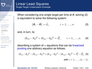
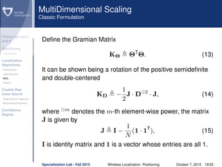
Preliminaries Definitions
{θa1
, · · ·, θaN
} is the ordered coordinate vectors of the aN
known nodes (a-priori known location).
{θ1, · · ·, θnT
} is the ordered coordinate vectors of the nT
target nodes (unknown location).
ΦA = [φa1
, · · · , φηaN
]T
and Φ = [φ1, · · · , φηnT
]T
are the
stacked vectors whose first and second nT elements are
given by {θi:x} and {θi:y}, respectively, where T
denotes
transpose.
dij θi − θj = θi − θj, θi − θj is the true distance
between the i-th and j-th nodes.
eij ∼ N(0, σ2
ij) is the Gaussian ranging error on the
distance estimate between the i-th and j-th nodes.
˜dij = dij + eij is the measured distance
Specialization Lab - Fall 2015 Wireless Localization: Positioning October 7, 2015 7/33](https://image.slidesharecdn.com/lecture032015-160126091341/85/Wireless-Localization-Positioning-7-320.jpg)


![Follow-Up Lect I
and II
Positioning
Preliminaries
Localization
Algorithms
Preliminaries
Least Squares
MDS
Smacof
Cramèr-Rao
lower bound
Target Specific Approach
Bidimensional Scenario
Confidence
Degree
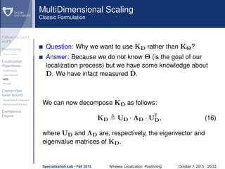
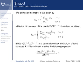
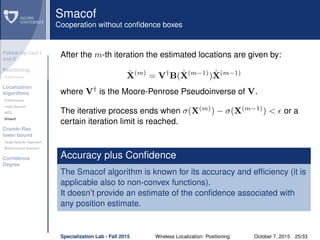
Smacof
Cooperation without confidence box
σ(X(0)
) = i<j wij( ˆd
(0)
ij − ˜dij)2
is the original stress function
ˆd
(m)
ij is the estimated distance dij after the m-th iteration
ˆX(m)
is the estimate of X = [Φ; ΦA] after the m-th iteration
ˆX(m−1)
is the solution at the previous iteration
τ( ˆX(m)
, ˆX(m−1)
) is the majored convex function at the m-th iteration
The majorized convex function
This algorithm attempts to find the minimum of a non-convex function by
majorizing the initial stress function and then tracking the global minimum
of the so-called majorized convex function τ( ˆX(m)
, ˆX(m-1)
) ,which is then
successively constructed from the previous solution ˆX(m-1)
obtained in the
iterative procedure.
The expression of the majorized convex function is:
τ( ˆX(m)
, ˆX(m−1)
) = 1+tr ˆX(m)T
V ˆX(m)
−2tr ˆX(m)T
B( ˆX(m−1)
) ˆX(m−1)
Specialization Lab - Fall 2015 Wireless Localization: Positioning October 7, 2015 23/33](https://image.slidesharecdn.com/lecture032015-160126091341/85/Wireless-Localization-Positioning-23-320.jpg)


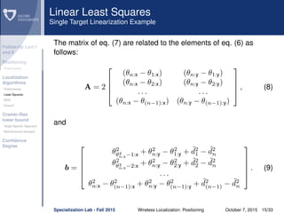
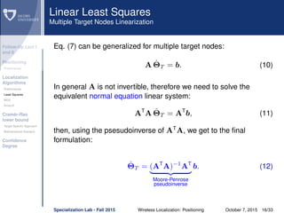
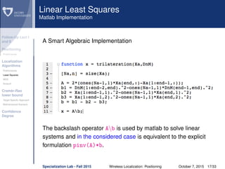
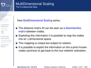
The document discusses wireless localization techniques focusing on positioning algorithms and the impacts of ranging error on target estimation accuracy. It highlights methods such as least squares, multidimensional scaling, and emphasizes the challenges arising from errors in distance measurements. The presentation also covers network types, algorithms for solving nonlinear systems, and a theoretical foundation for enhanced localization strategies.