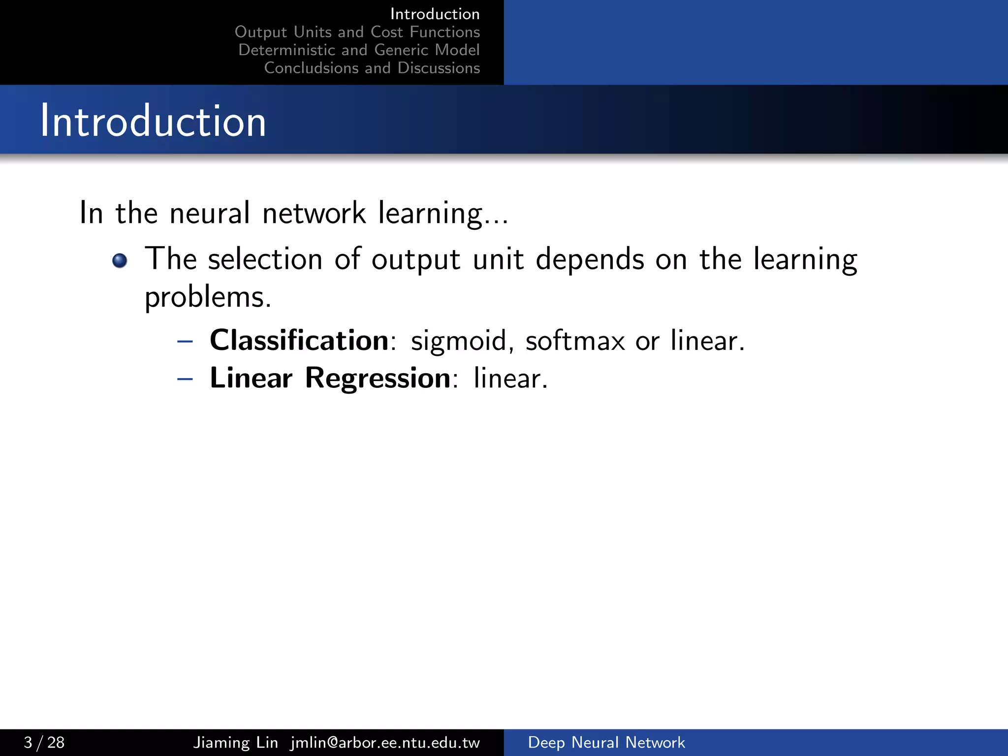
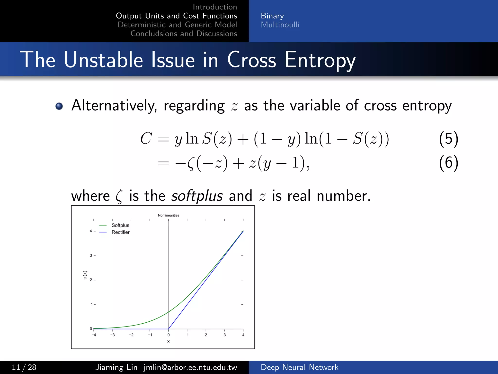
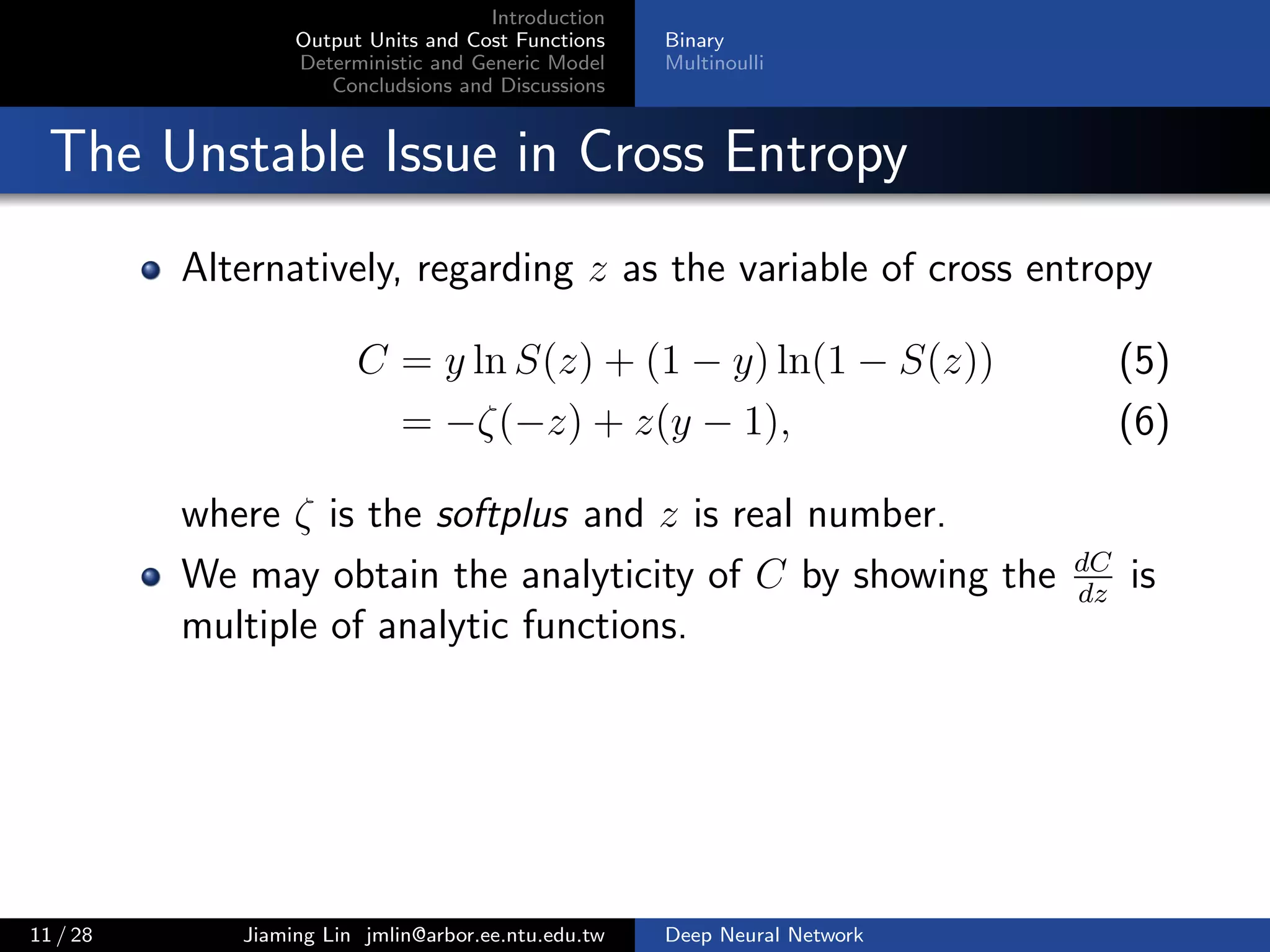
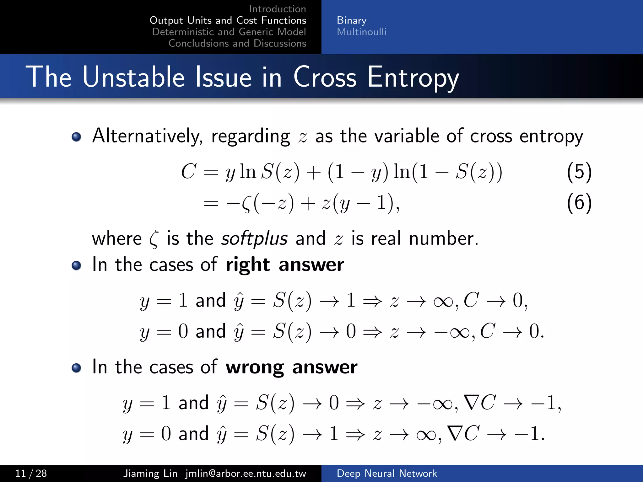
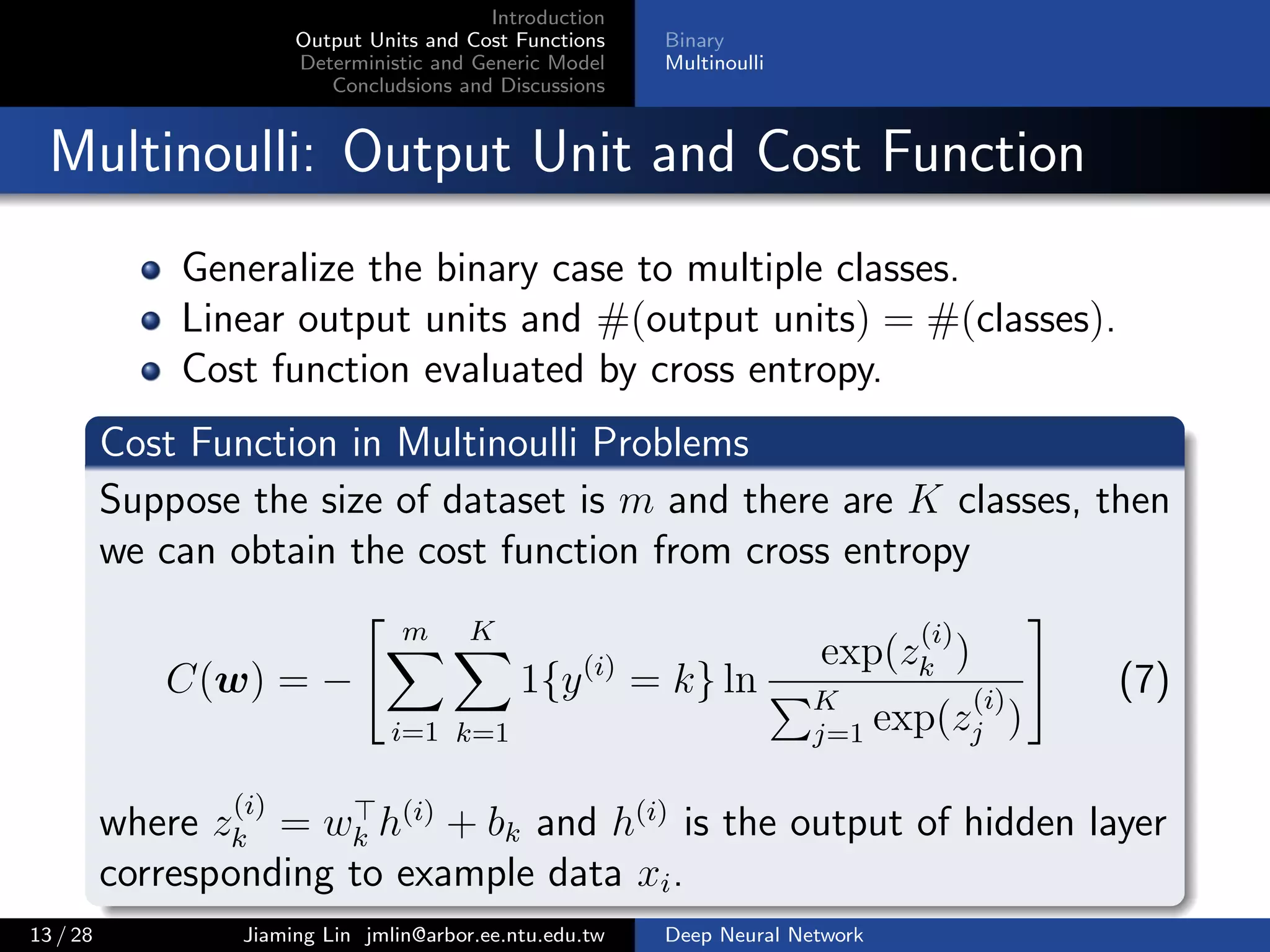
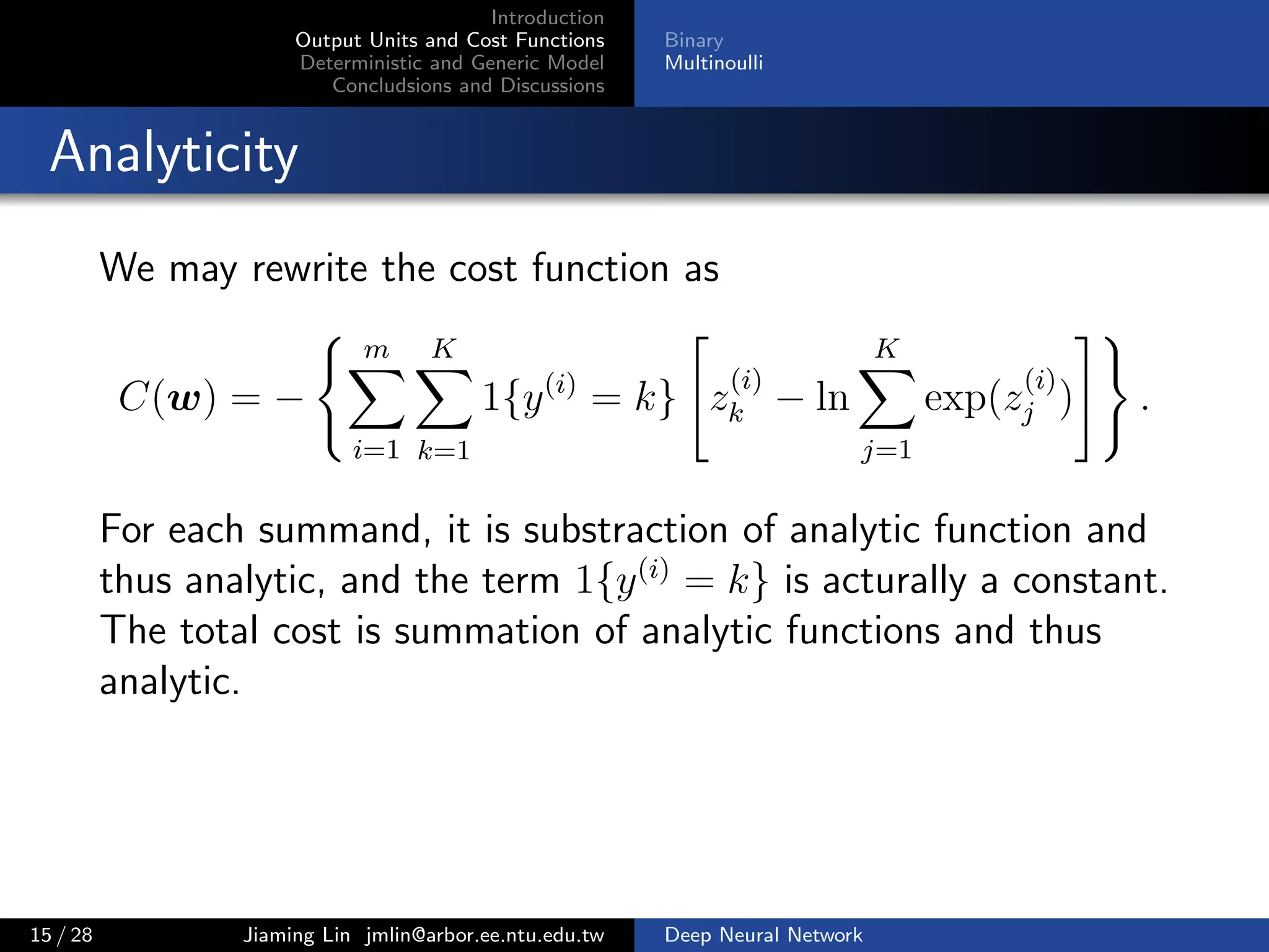
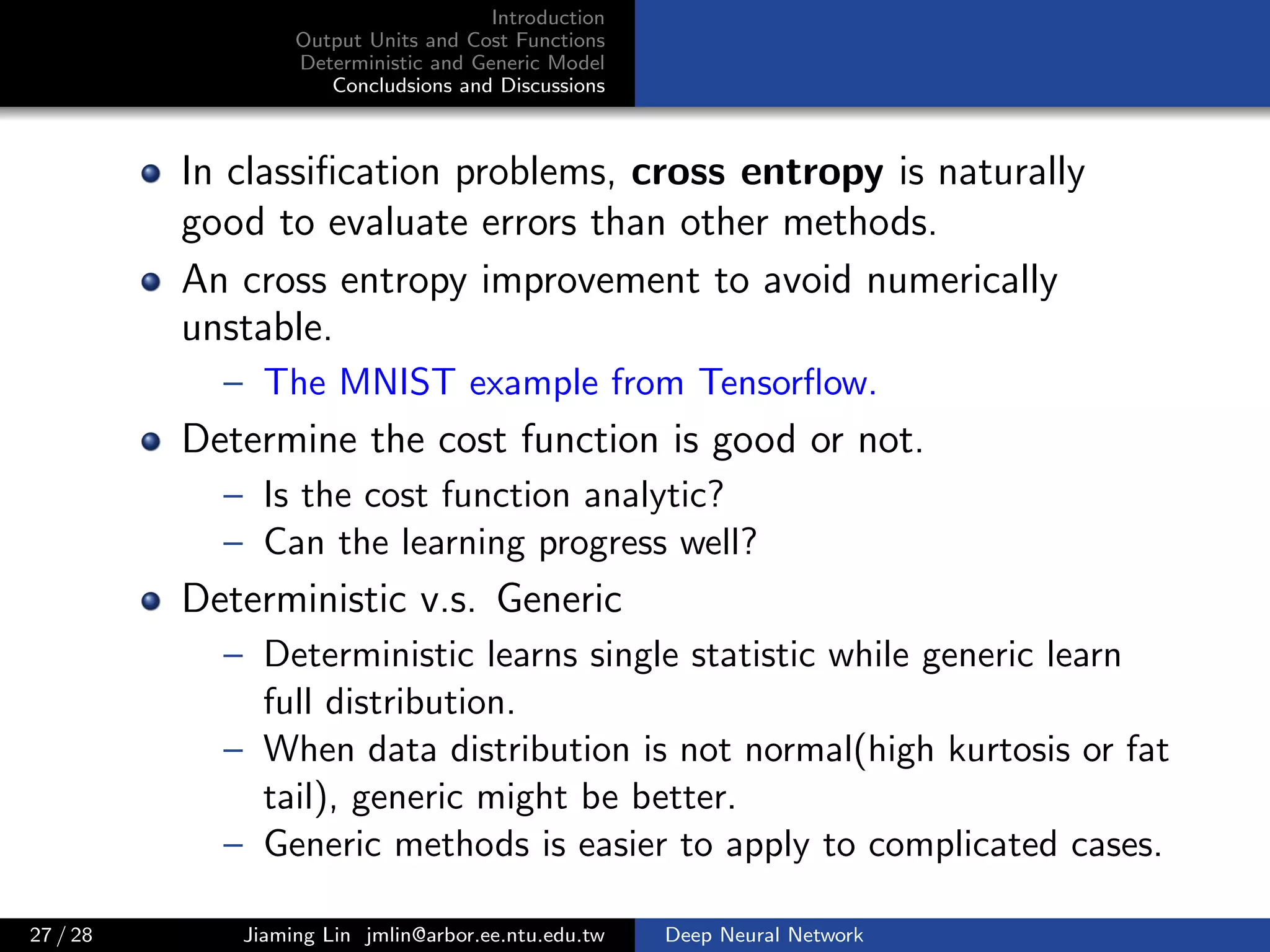
The document discusses the selection of output units and cost functions in deep neural networks, emphasizing criteria for classification and regression tasks. It evaluates two predominant cost functions: mean square error and cross entropy, comparing their analyticity and learning ability. The document further extends the discussion to multinoulli classification, detailing the cost function derivation and properties necessary for efficient learning and function stability.


![Introduction
Output Units and Cost Functions
Deterministic and Generic Model
Concludsions and Discussions
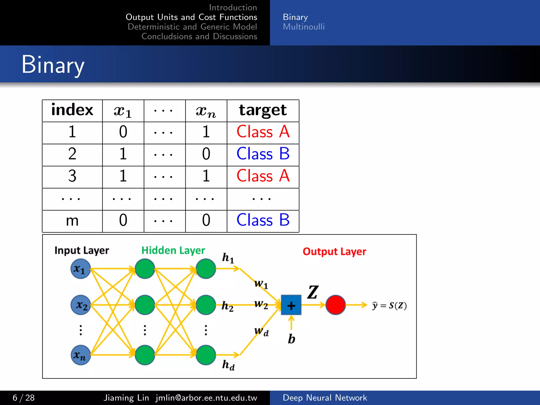
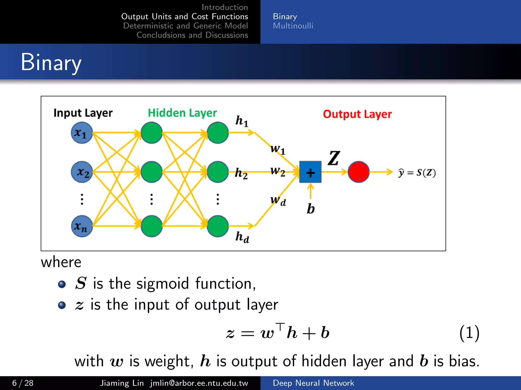
Binary
Multinoulli
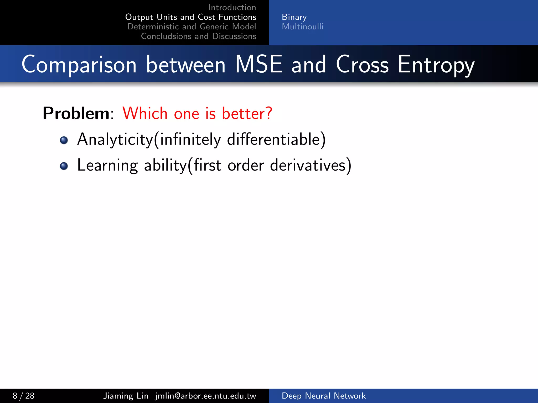
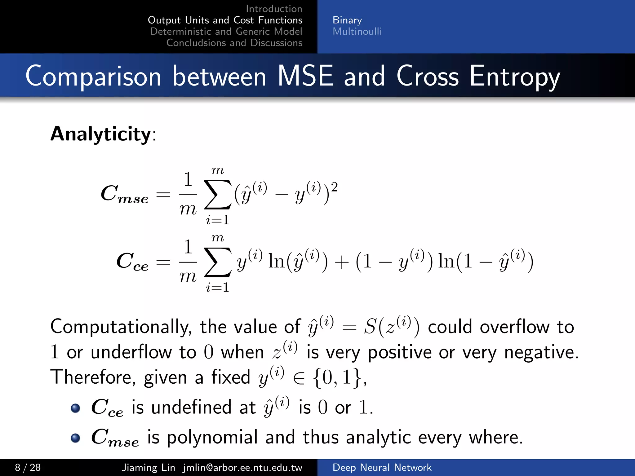
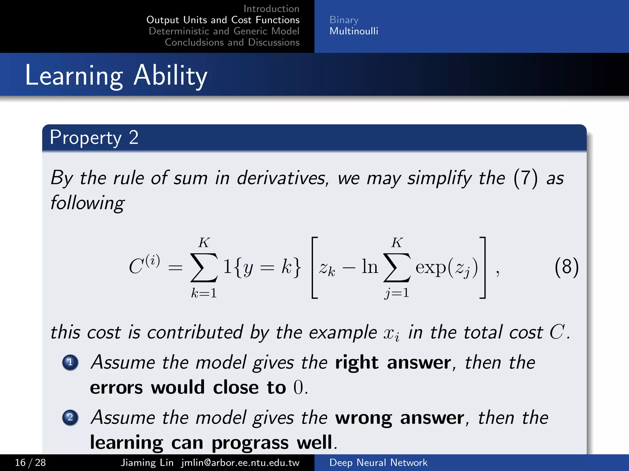
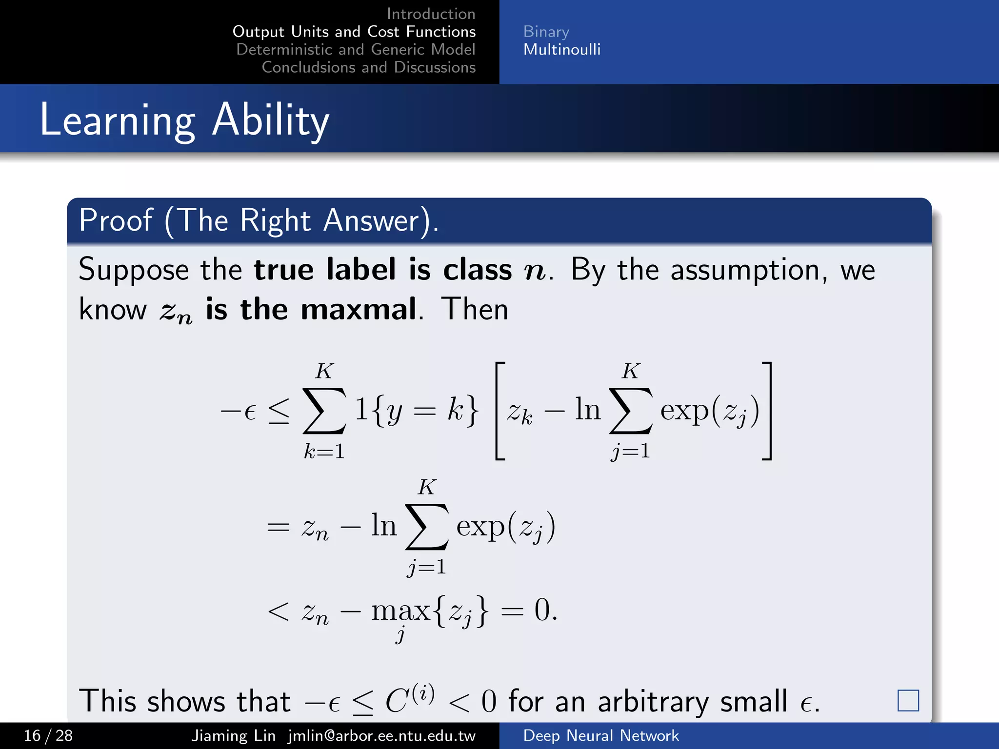
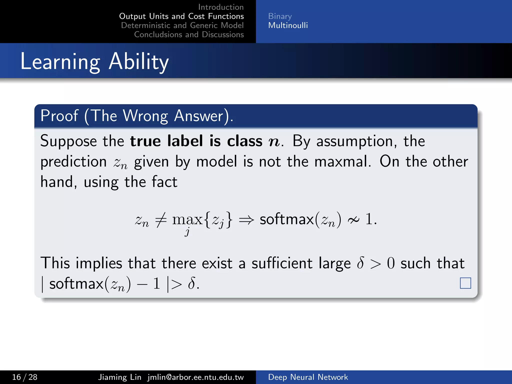
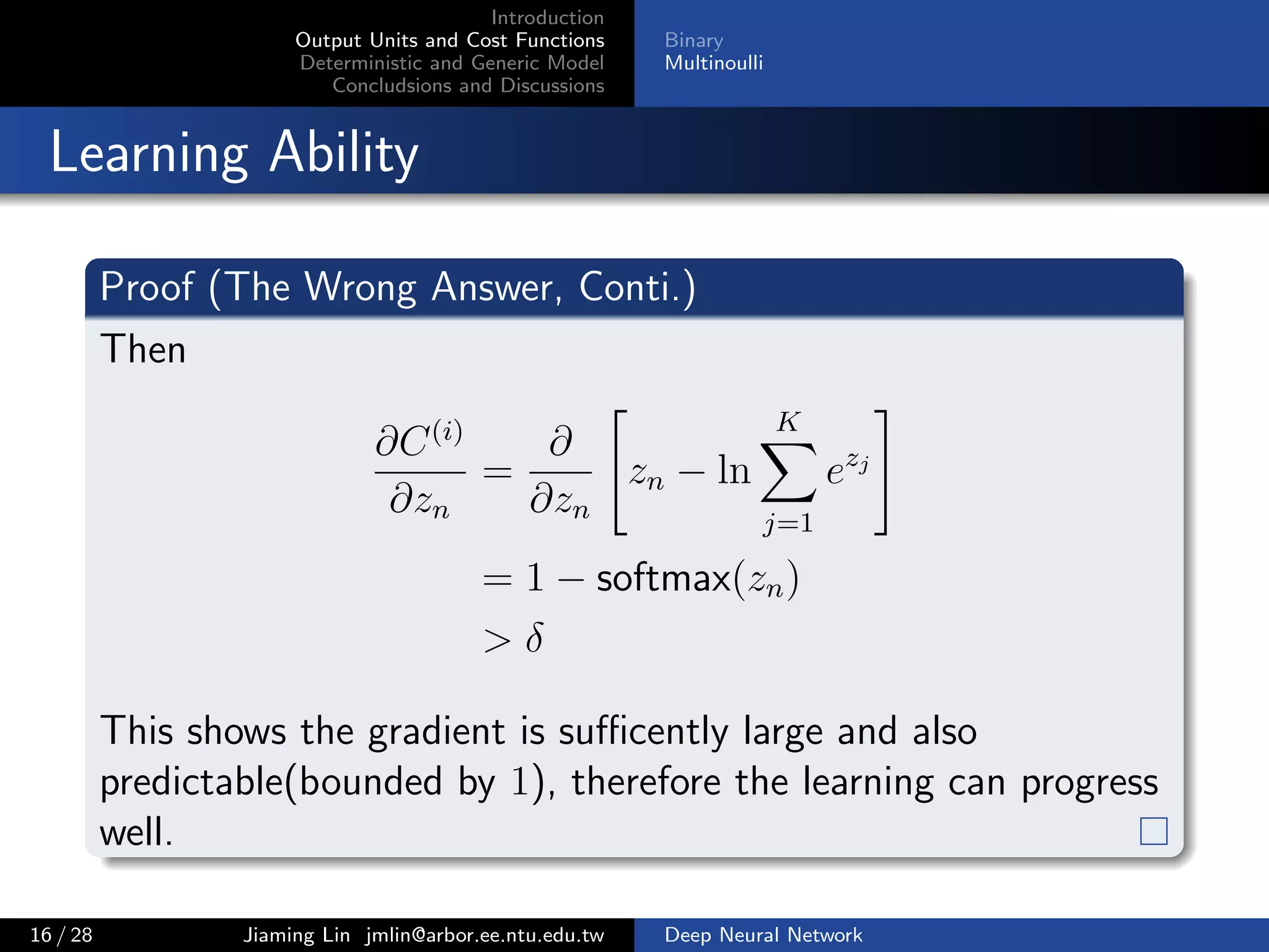
Comparison between MSE and Cross Entropy
Learning Ability: compare the gradients
∂Cmse
∂w
= [S(z) − y] [1 − S(z)] S(z)h, (3)
∂Cce
∂w
= [y − S(z)] h (4)
respectively, where S is sigmoid, z = w h + b.
8 / 28 Jiaming Lin jmlin@arbor.ee.ntu.edu.tw Deep Neural Network](https://image.slidesharecdn.com/fnnoutputcost-170109103653/75/Output-Units-and-Cost-Function-in-FNN-15-2048.jpg)
![Introduction
Output Units and Cost Functions
Deterministic and Generic Model
Concludsions and Discussions
Binary
Multinoulli
Comparison between MSE and Cross Entropy
MSE Cross Entropy
[S(z) − y] [1 − S(z)] S(z)h [y − S(z)] h
If y = 1 and ˆy → 1,
steps → 0
If y = 1 and ˆy → 0,
steps → 0
If y = 0 and ˆy → 1,
steps → 0
If y = 0 and ˆy → 0,
steps → 0
If y = 1 and ˆy → 1,
steps → 0
If y = 1 and ˆy → 0,
steps → 1
If y = 0 and ˆy → 1,
steps → −1
If y = 0 and ˆy → 0,
steps → 0
9 / 28 Jiaming Lin jmlin@arbor.ee.ntu.edu.tw Deep Neural Network](https://image.slidesharecdn.com/fnnoutputcost-170109103653/75/Output-Units-and-Cost-Function-in-FNN-16-2048.jpg)
![Introduction
Output Units and Cost Functions
Deterministic and Generic Model
Concludsions and Discussions
Binary
Multinoulli
Comparison between MSE and Cross Entropy
MSE Cross Entropy
[S(z) − y] [1 − S(z)] S(z)h [y − S(z)] h
If y = 1 and ˆy → 1,
steps → 0
If y = 1 and ˆy → 0,
steps → 0
If y = 0 and ˆy → 1,
steps → 0
If y = 0 and ˆy → 0,
steps → 0
If y = 1 and ˆy → 1,
steps → 0
If y = 1 and ˆy → 0,
steps → 1
If y = 0 and ˆy → 1,
steps → −1
If y = 0 and ˆy → 0,
steps → 0
In the ceas of Mean Square Error, the progress get stuck when
z is very positive or very negative.
9 / 28 Jiaming Lin jmlin@arbor.ee.ntu.edu.tw Deep Neural Network](https://image.slidesharecdn.com/fnnoutputcost-170109103653/75/Output-Units-and-Cost-Function-in-FNN-17-2048.jpg)

![Introduction
Output Units and Cost Functions
Deterministic and Generic Model
Concludsions and Discussions
Binary
Multinoulli
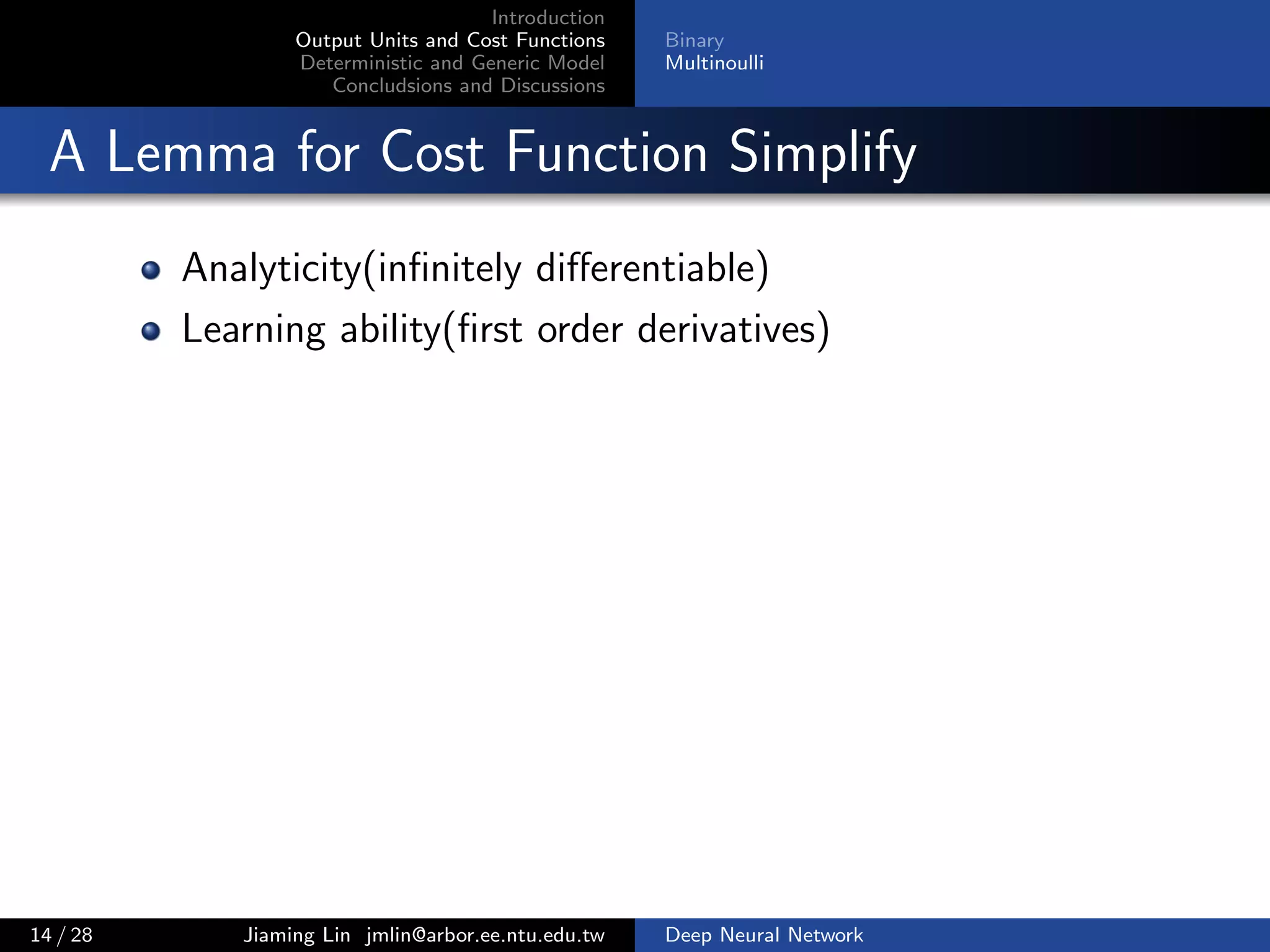
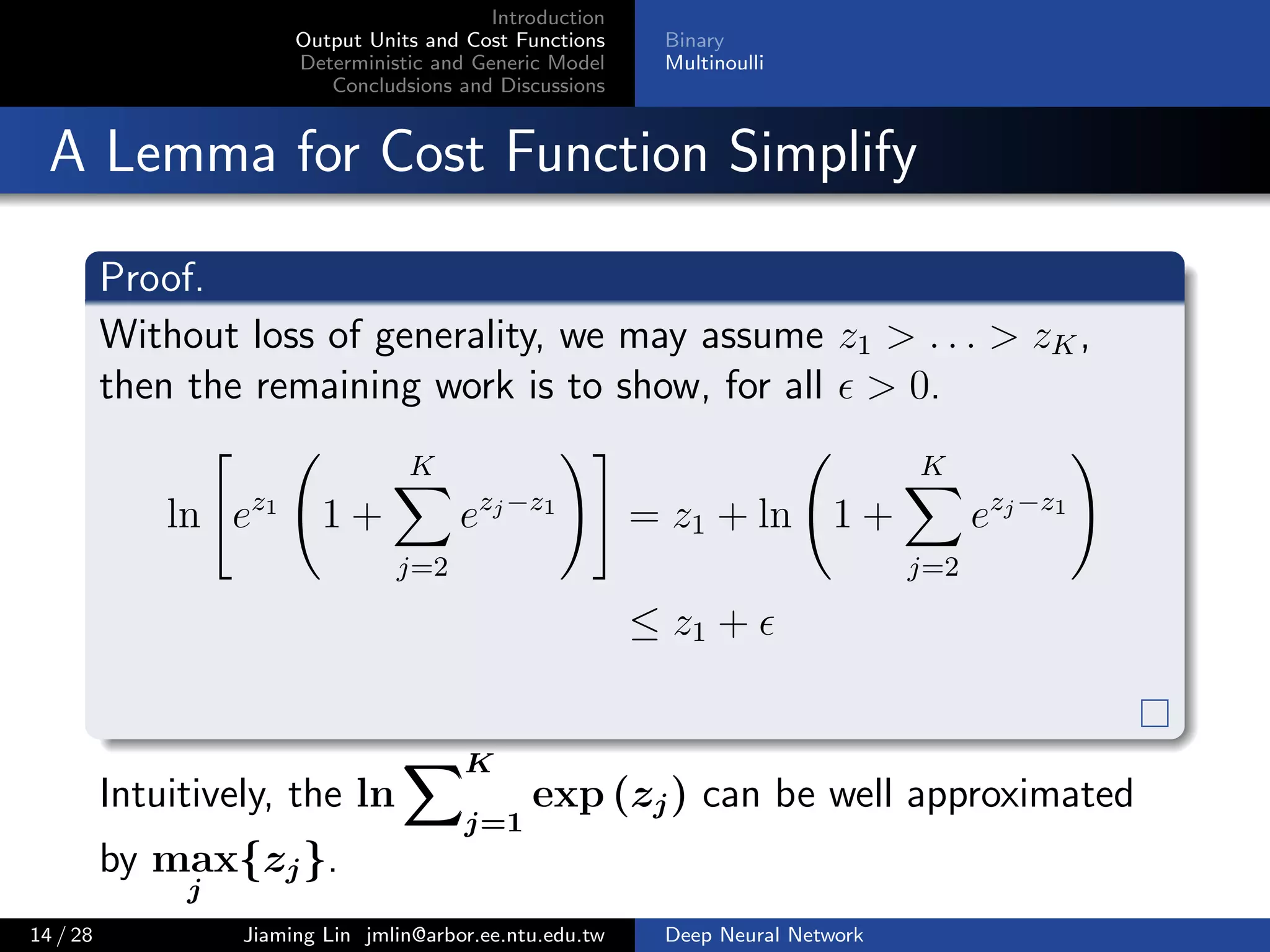
A Lemma for Cost Function Simplify
Analyticity(infinitely differentiable)
Learning ability(first order derivatives)
To claim above properties, We should show a lemma at very
first,
Lemma 1
For the output z = w h + b and z = [z1, . . . , zK], we have
sup
z
ln
K
j=1
exp(zj) = max
j
{zj}. (8)
14 / 28 Jiaming Lin jmlin@arbor.ee.ntu.edu.tw Deep Neural Network](https://image.slidesharecdn.com/fnnoutputcost-170109103653/75/Output-Units-and-Cost-Function-in-FNN-27-2048.jpg)

![Introduction
Output Units and Cost Functions
Deterministic and Generic Model
Concludsions and Discussions
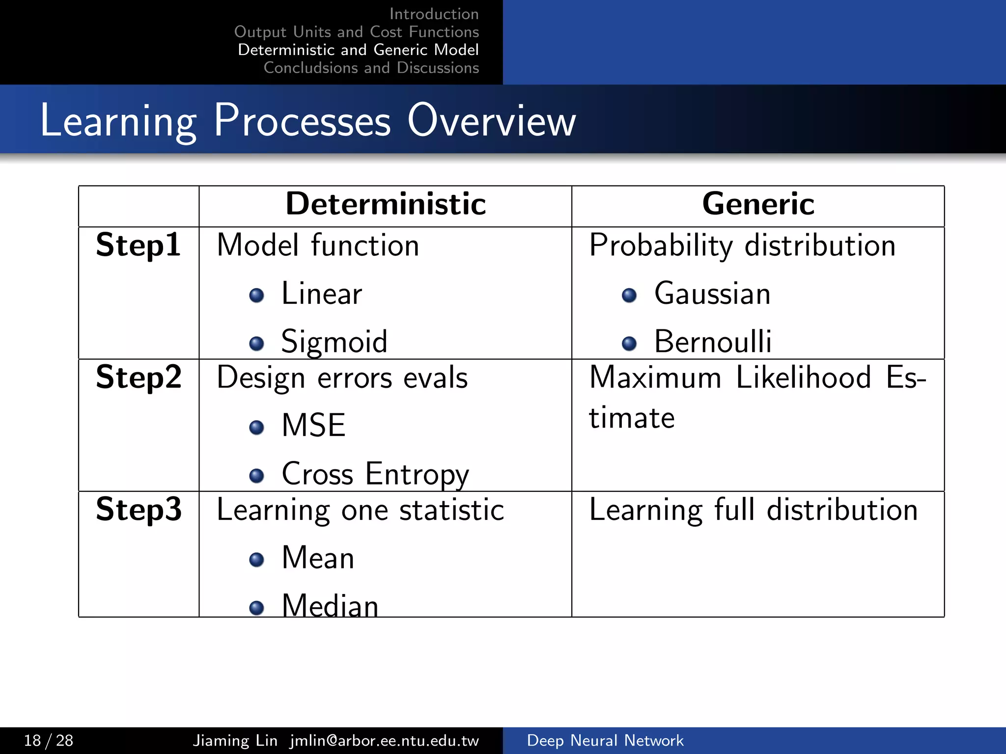
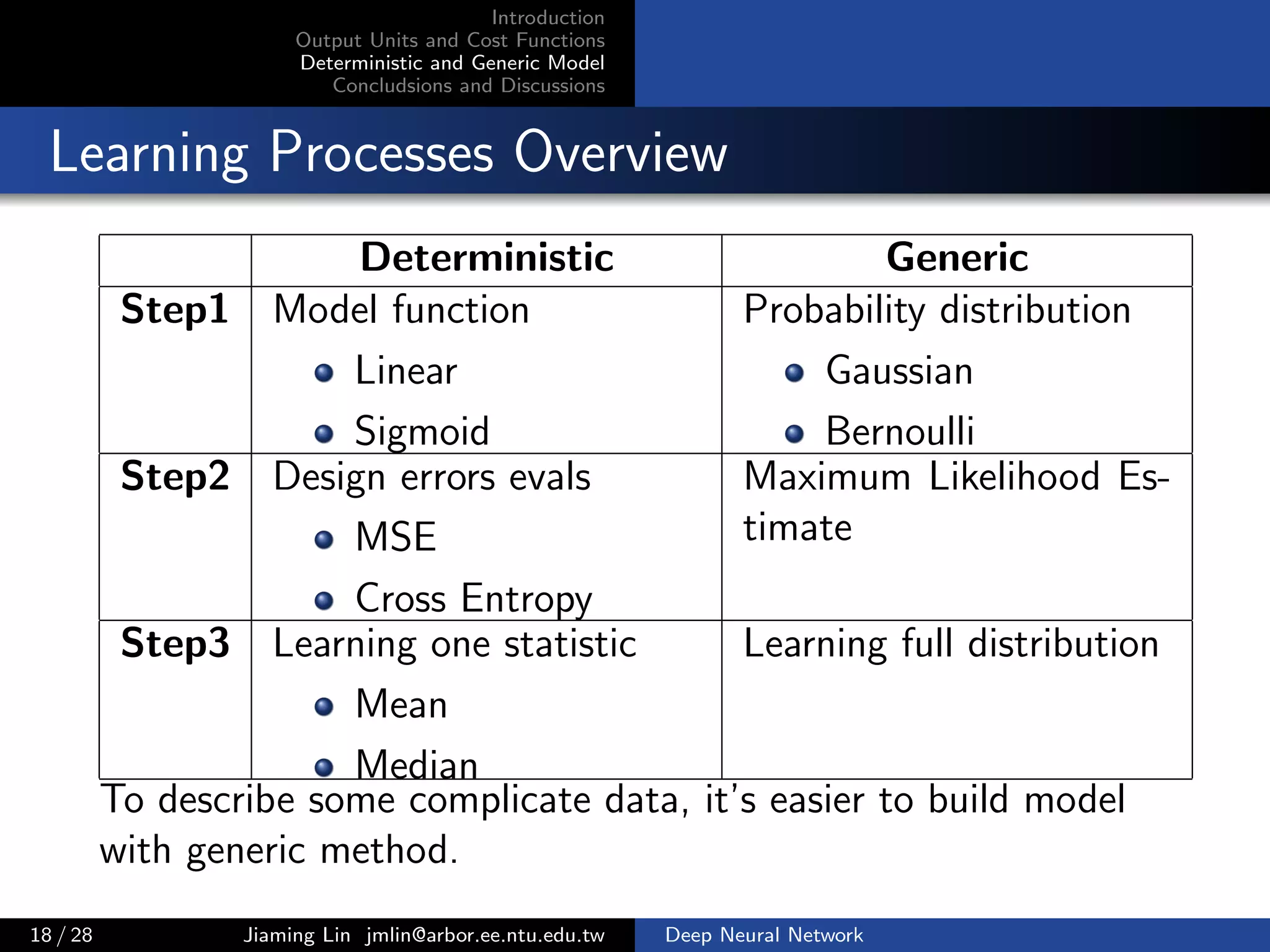
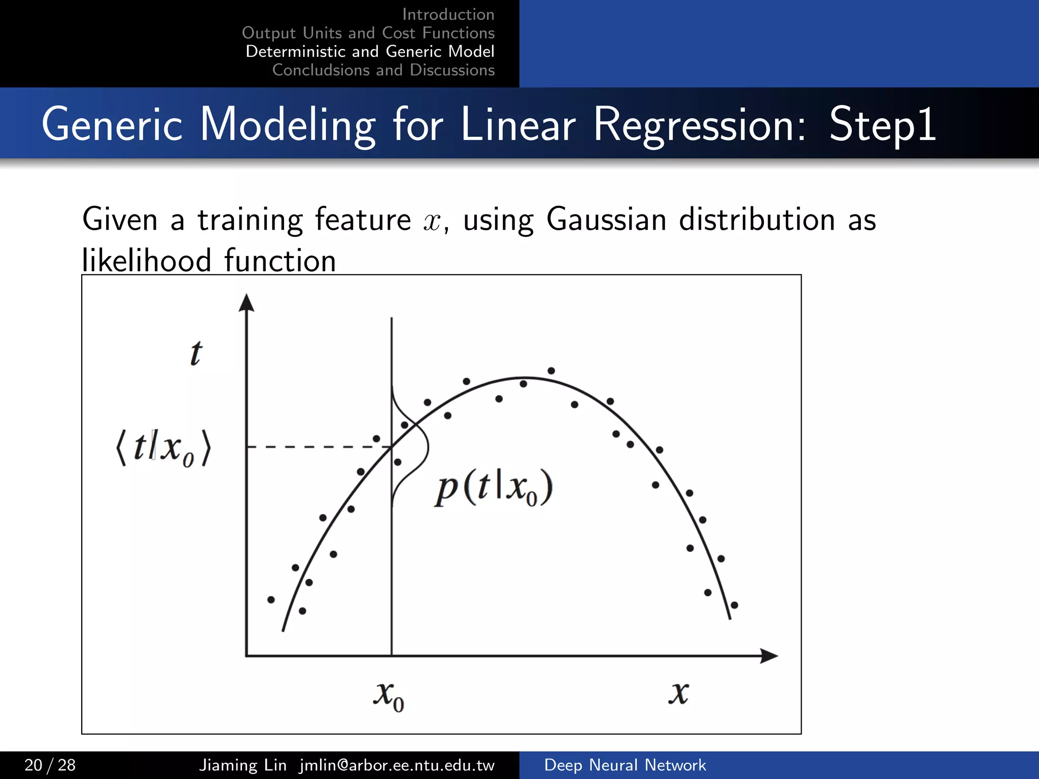
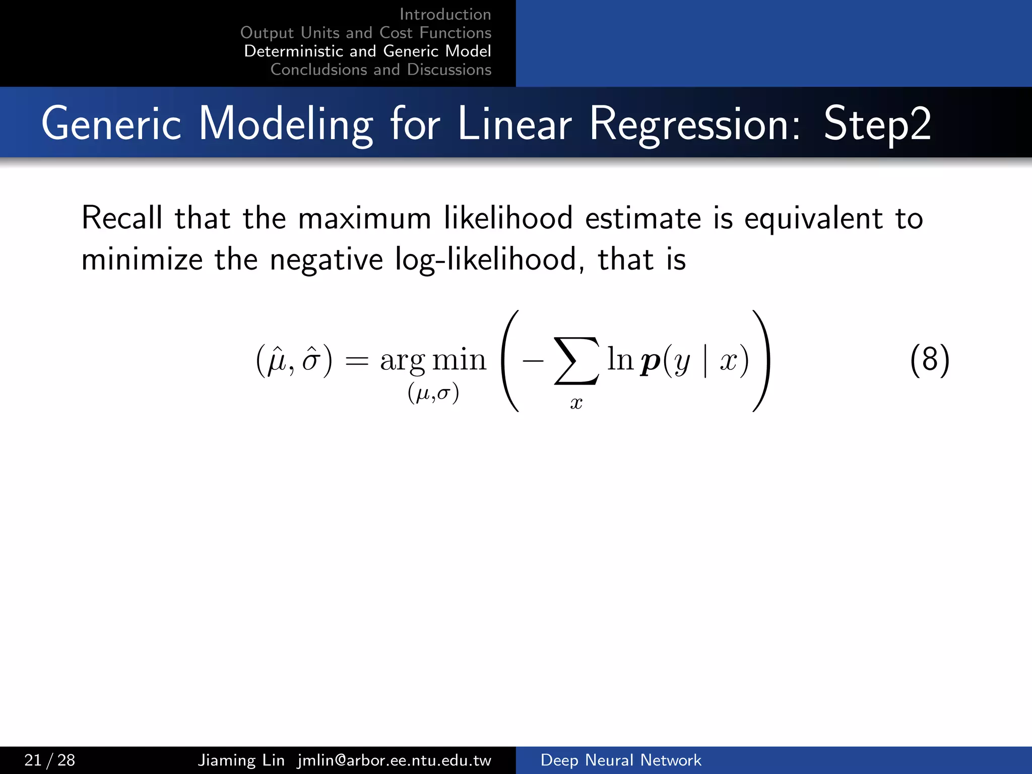
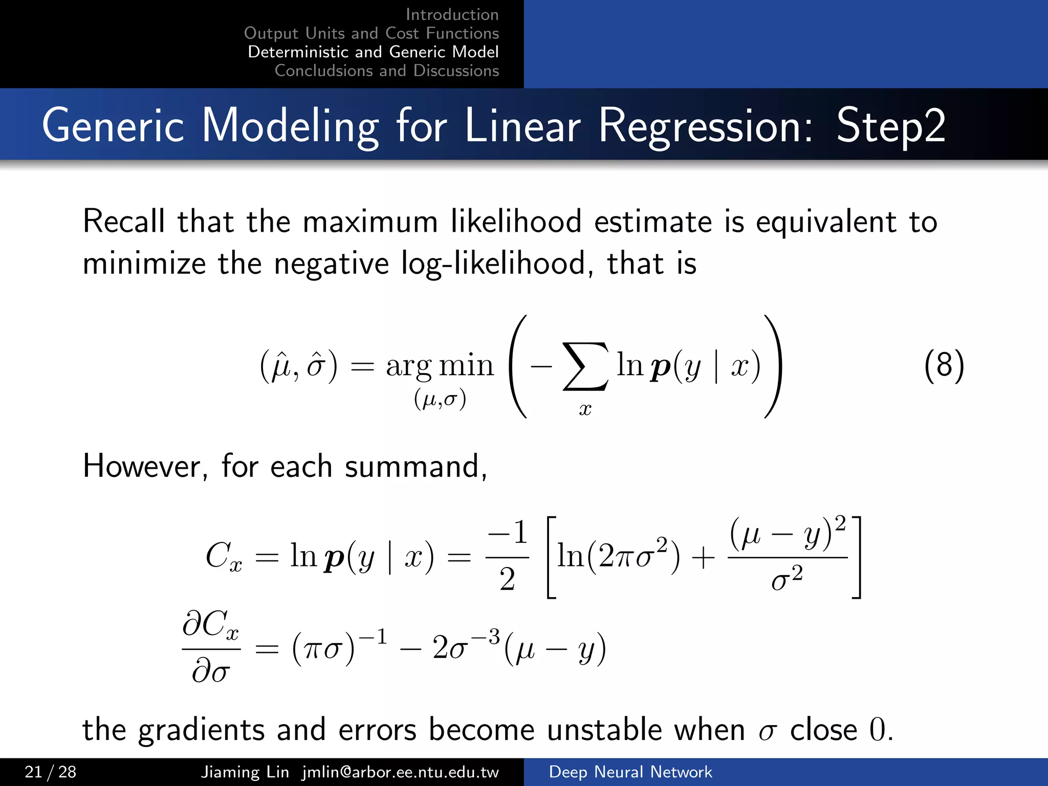
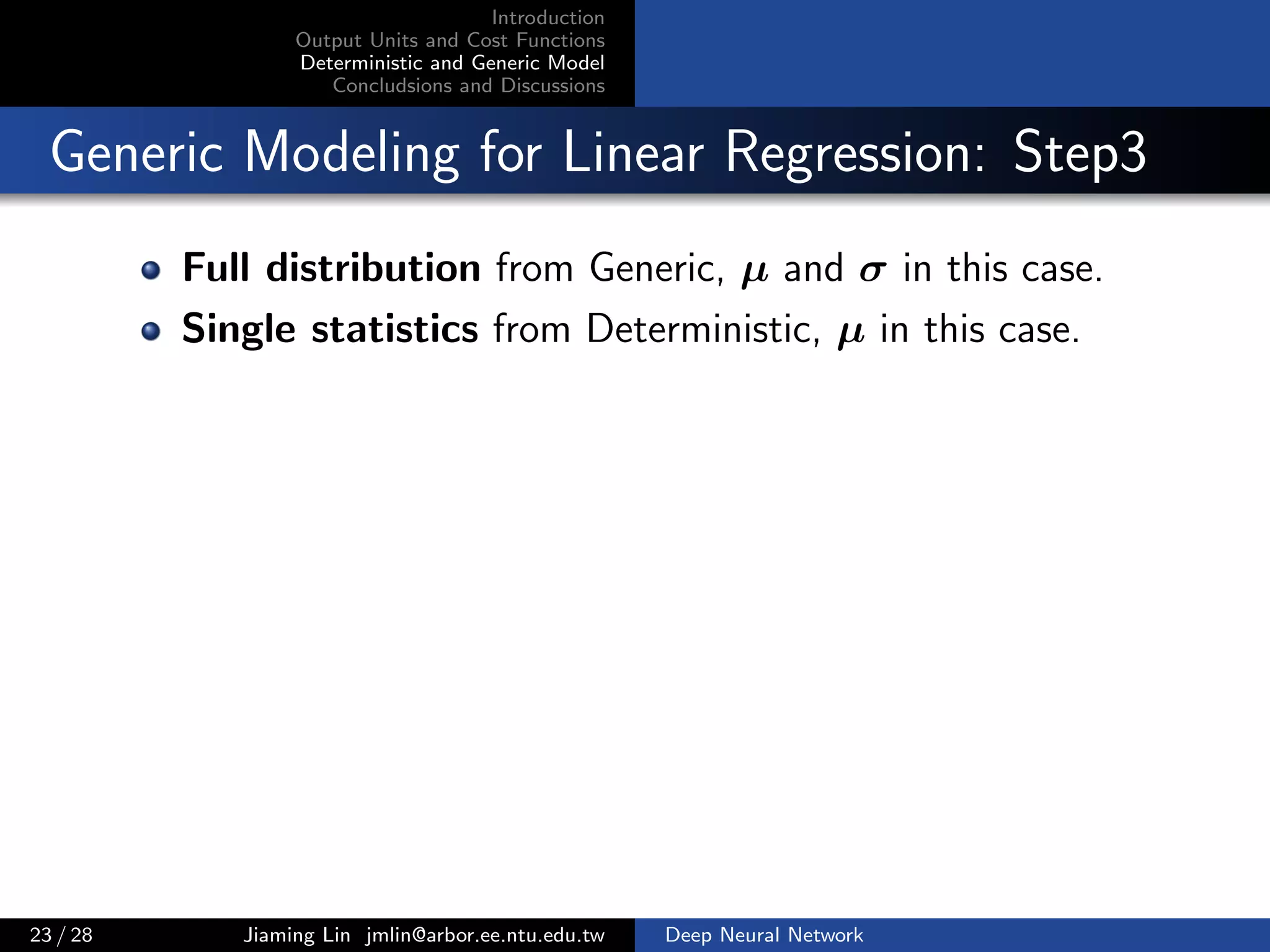
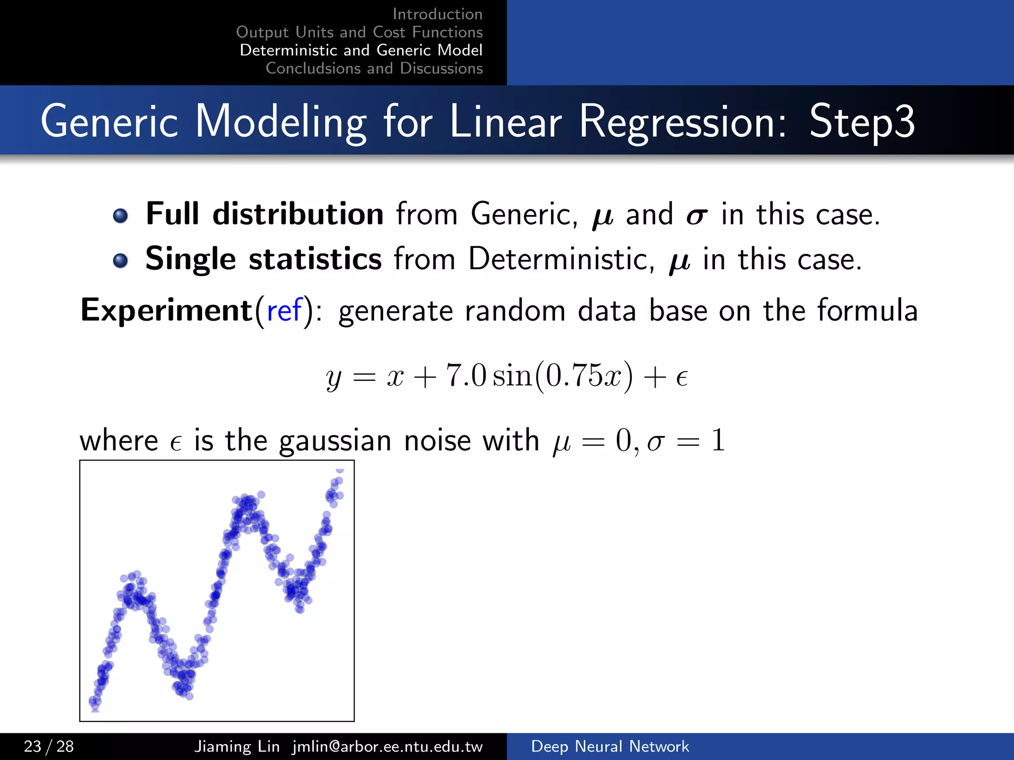
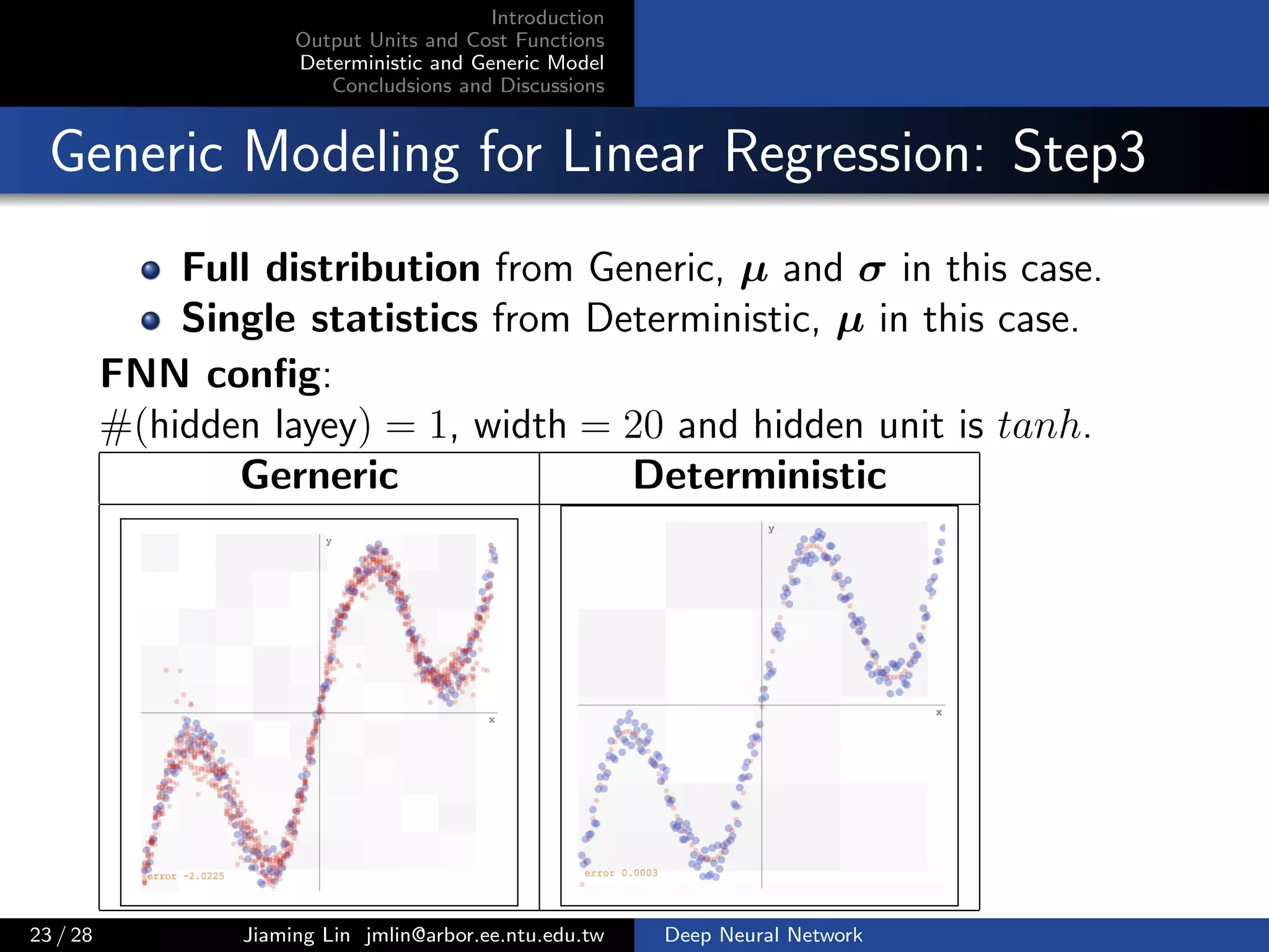
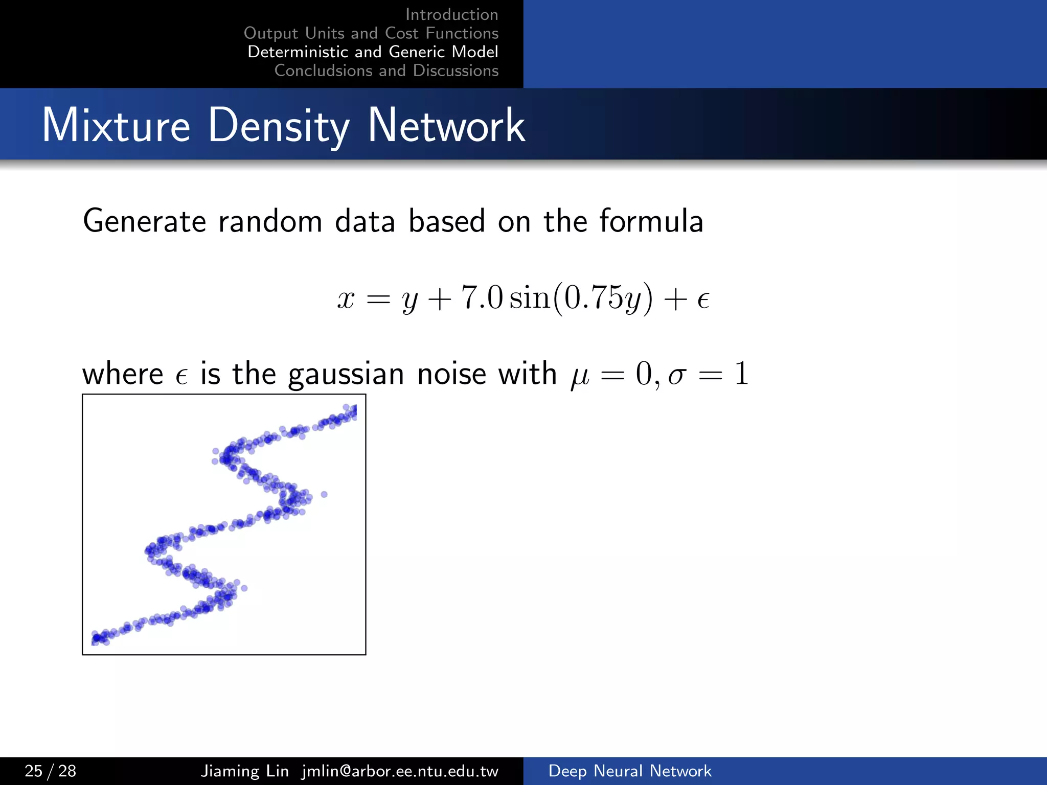
Generic Modeling for Linear Regression: Step1
Given a training feature x, using Gaussian distribution as
likelihood function
p(y | x) =
1
√
2σ2π
exp
−(µ − y)2
2σ2
,
where we denote the output of hidden layer as hx, weight
w = [w1, w2] and bias b = [b1, b2], then
µ = w1 hx + b1
σ = w2 hx + b2
Intuitively, µ and σ are two linear output units, they are
functions of x.
20 / 28 Jiaming Lin jmlin@arbor.ee.ntu.edu.tw Deep Neural Network](https://image.slidesharecdn.com/fnnoutputcost-170109103653/75/Output-Units-and-Cost-Function-in-FNN-39-2048.jpg)


![Lec 9 05_sept [compatibility mode]](https://cdn.slidesharecdn.com/ss_thumbnails/lec905septcompatibilitymode-130917013819-phpapp01-thumbnail.jpg?width=640&height=640&fit=bounds)


![[DSC 2016] 系列活動:李宏毅 / 一天搞懂深度學習](https://cdn.slidesharecdn.com/ss_thumbnails/1-160521014039-thumbnail.jpg?width=640&height=640&fit=bounds)


![[DSC Europe 25] Jovan Bogicevic - Legacy to AI-Driven Defense: Transforming D...](https://cdn.slidesharecdn.com/ss_thumbnails/rsarluadt563hntyfc8q-3-251211083849-3e7bc4c0-thumbnail.jpg?width=640&height=640&fit=bounds)

![[DSC Europe 25] Branko Urosevic -Rethinking Financial Talent: Integrating Cod...](https://cdn.slidesharecdn.com/ss_thumbnails/8jjrus8ttko6qj64f58f-3-251212103250-642c6374-thumbnail.jpg?width=640&height=640&fit=bounds)
![[DSC Europe 25] Dragana Ilic - AI for Big Data in Astronomy.pptx](https://cdn.slidesharecdn.com/ss_thumbnails/8palya86qaatvjhva1ms-2-dragana-ilic-ai-ilic-251208151906-652b819c-thumbnail.jpg?width=640&height=640&fit=bounds)
![[DSC Europe 25] Dusan Nesic - Securing Tomorrow’s Infrastructure: Why Cyber-P...](https://cdn.slidesharecdn.com/ss_thumbnails/qikbszfftyowjm2q6duw-1-251211083848-8f2ead6b-thumbnail.jpg?width=640&height=640&fit=bounds)
![[DSC Europe 25] Jon Dajci - Bridging TradFi and DeFi: Building the Future of ...](https://cdn.slidesharecdn.com/ss_thumbnails/fqmhfvlbqhkihjvqvhmu-7-251211083849-6af7e325-thumbnail.jpg?width=640&height=640&fit=bounds)
![[DSC Europe 25] Marko Krstic - Understanding the AI Threat Landscape - Risks,...](https://cdn.slidesharecdn.com/ss_thumbnails/tiyim1ins5jvbrvzpzla-2-251209104645-c69d3553-thumbnail.jpg?width=640&height=640&fit=bounds)
![[DSC Europe 25] Vladimir Jelic - The AI-Driven Security Shift From Reactive D...](https://cdn.slidesharecdn.com/ss_thumbnails/6g5gj25mtjwayniqem1t-6-251209104645-7a5a5fc6-thumbnail.jpg?width=640&height=640&fit=bounds)


![[DSC Europe 25] Milan Zdravkovic - The road less traveled in District Heating...](https://cdn.slidesharecdn.com/ss_thumbnails/nfaboniqwsz4ucyctnmy-2-milan-zdravkovic-dsc2025-the-road-less-traveled-in-district-heating-operation-251208151905-f56388a5-thumbnail.jpg?width=640&height=640&fit=bounds)

![[DSC Europe 25] Marija Vlajkovic & Andrea Radonjanin - Integration of AI tool...](https://cdn.slidesharecdn.com/ss_thumbnails/qf1jrglttoc3bm8s3aop-final-integration-of-ai-tools-251208151905-394f3a6a-thumbnail.jpg?width=640&height=640&fit=bounds)

![[DSC Europe 25] Sara Polak - The Ancient Operating System: What Archaeology T...](https://cdn.slidesharecdn.com/ss_thumbnails/3vch2p6tttdnwhsgazoz-3-sara-polak-smart-cities-251208152532-64404202-thumbnail.jpg?width=640&height=640&fit=bounds)
![[DSC Europe 25] Sara Polak - The Archaeology of Innovation: AI as the Next Cr...](https://cdn.slidesharecdn.com/ss_thumbnails/7ecbscdnt8mlcuqbd2ln-2-sara-polak-ai-creative-industries-251208152533-aa1fcf54-thumbnail.jpg?width=640&height=640&fit=bounds)
![[DSC Europe 25] Katherine Forrest - AI NOW: Understanding the Velocity of Cha...](https://cdn.slidesharecdn.com/ss_thumbnails/wvvbruqfrci0sfq9xwgb-4-251212104007-e5ad1987-thumbnail.jpg?width=640&height=640&fit=bounds)