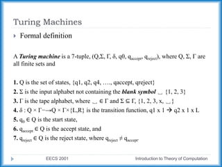
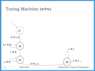
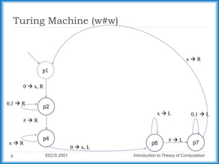
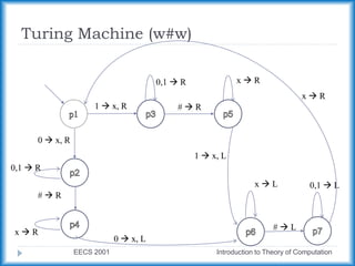
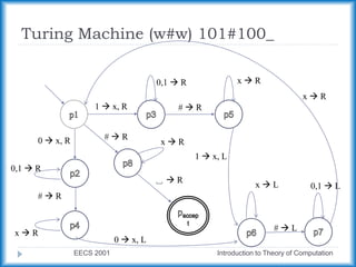
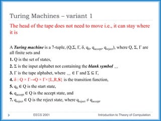
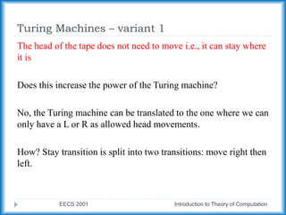
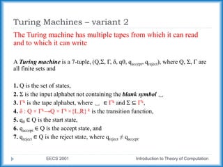
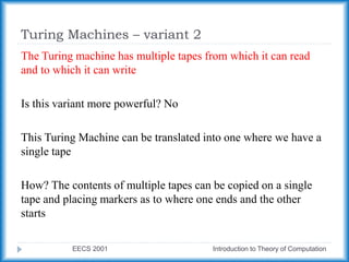
EECS 2001: Introduction to the
Theory of Computation
Muhammad Umair Khan
Turing Machines
EECS 2001 Introduction to Theory of Computation
 Unlimited memory
 Very close to the current computers
Turing Machines
EECS 2001 Introduction to Theory of Computation
 Unlimited memory
 Very close to the current computers
 Comparing with FA
 Write onto and read from a tape
 Read-write head can move both to the left or right on the tape (no
limitations of stack and queue)
 Tape is memory which is infinite
 Accept and reject states
Turing Machines
EECS 2001 Introduction to Theory of Computation
 Formal definition
A Turing machine is a 7-tuple, (Q,Σ, Γ, δ, q0, qaccept, qreject), where Q, Σ, Γ are
all finite sets and
1. Q is the set of states, {q1, q2, q4, …., qaccept, qreject}
2. Σ is the input alphabet not containing the blank symbol ␣ {1, 2, 3}
3. Γ is the tape alphabet, where ␣ ∈ Γ and Σ ⊆ Γ, {1, 2, 3, x, ␣}
4. δ : Q × Γ−→Q × Γ×{L,R} is the transition function, q1 x 1  q2 x 1 x L
5. q0 ∈ Q is the start state,
6. qaccept ∈ Q is the accept state, and
7. qreject ∈ Q is the reject state, where qreject ≠ qaccept.
Turing Machines
EECS 2001 Introduction to Theory of Computation
 Input words are on the leftmost places on the tape
 Remaining tape is blank
 At the beginning, the read /write head is on the leftmost place on the tape
 A blank symbol will indicate the end of input as the blank symbol is not part
of the input alphabet
 Moving left from the leftmost place keeps you in the same place
 As the Turing machine processes, the contents of the tape change
 Current state, current location of the head, and current contents of the tape
constitute the configuration of the Turing machine.
Turing Machines
EECS 2001 Introduction to Theory of Computation
 Consider the language B = {w#w| w ∈ {0,1}*} i.e., two
identical strings separated by a #
 The algorithms using a Turing machine will look as follows
Zig-zag across the tape to corresponding positions on either side of the # symbol to
check whether these positions contain the same symbol. If they do not, or if no # is
found, reject. Cross off symbols as they are checked to keep track of which symbols
correspond.
When all symbols to the left of the # have been crossed off, check for any remaining
symbols to the right of the #. If any symbols remain, reject; otherwise, accept .
Turing Machines
EECS 2001 Introduction to Theory of Computation
 Consider the language B = {w#w| w ∈ {0,1}*} i.e., two
identical strings separated by a #
Turing Machines
EECS 2001 Introduction to Theory of Computation
 Formal Definition of M which recognizes B = {w#w| w ∈
{0,1}*}
 Q = {p1, . . . , p8, paccept, preject},
 Σ = {0, 1, #}, and Γ = {0, 1, #, x, ␣}.
 We describe δ with a state diagram (see the following figure).
 The start, accept, and reject states are p1, paccept, and preject,
respectively.
Turing Machine (w#w)
EECS 2001 Introduction to Theory of Computation
x  L
0  x, R
0  x, L
0,1  R
x  R
#  R
#  L
Turing Machine (w#w)
EECS 2001 Introduction to Theory of Computation
x  L
0  x, R
0  x, L
0,1  R
x  R
#  R
#  L
0,1  L
x  R
Turing Machine (w#w)
EECS 2001 Introduction to Theory of Computation
1  x, R
x  L
0  x, R
0  x, L
0,1  R
x  R
#  R
0,1  R
#  R
x  R
1  x, L
#  L
0,1  L
x  R
Turing Machine (w#w) 101#100_
EECS 2001 Introduction to Theory of Computation
1  x, R
x  L
0  x, R
0  x, L
0,1  R
x  R
#  R
0,1  R
#  R
x  R
#  R
1  x, L
#  L
0,1  L
␣  R
x  R
x  R
Turing Machines – variant 1
EECS 2001 Introduction to Theory of Computation
The head of the tape does not need to move i.e., it can stay where
it is
A Turing machine is a 7-tuple, (Q,Σ, Γ, δ, q0, qaccept, qreject), where Q, Σ, Γ are
all finite sets and
1. Q is the set of states,
2. Σ is the input alphabet not containing the blank symbol ␣
3. Γ is the tape alphabet, where ␣ ∈ Γ and Σ ⊆ Γ,
4. δ : Q × Γ→Q × Γ×{L,R,S} is the transition function,
5. q0 ∈ Q is the start state,
6. qaccept ∈ Q is the accept state, and
7. qreject ∈ Q is the reject state, where qreject ≠ qaccept.
Turing Machines – variant 1
EECS 2001 Introduction to Theory of Computation
The head of the tape does not need to move i.e., it can stay where
it is
Does this increase the power of the Turing machine?
No, the Turing machine can be translated to the one where we can
only have a L or R as allowed head movements.
How? Stay transition is split into two transitions: move right then
left.
Turing Machines – variant 2
EECS 2001 Introduction to Theory of Computation
The Turing machine has multiple tapes from which it can read
and to which it can write
A Turing machine is a 7-tuple, (Q,Σ, Γ, δ, q0, qaccept, qreject), where Q, Σ, Γ are
all finite sets and
1. Q is the set of states,
2. Σ is the input alphabet not containing the blank symbol ␣
3. Γk is the tape alphabet, where ␣ ∈ Γk and Σ ⊆ Γk,
4. δ : Q × Γk→Q × Γk ×{L,R} k is the transition function,
5. q0 ∈ Q is the start state,
6. qaccept ∈ Q is the accept state, and
7. qreject ∈ Q is the reject state, where qreject ≠ qaccept.
Turing Machines – variant 2
EECS 2001 Introduction to Theory of Computation
The Turing machine has multiple tapes from which it can read
and to which it can write
Is this variant more powerful? No
This Turing Machine can be translated into one where we have a
single tape
How? The contents of multiple tapes can be copied on a single
tape and placing markers as to where one ends and the other
starts
Turing Machines – variant 2
EECS 2001 Introduction to Theory of Computation
The Turing machine has multiple tapes from which it can read
and to which it can write
δ (qi, a1, …, ak) = (qj, b1, …, bk, L, R, L, …., L)
Turing Machines – variant 3
EECS 2001 Introduction to Theory of Computation
Two-way Infinite Tape Turing Machines
Number the cells on the tape as … -3, -2, -1, 0, 1, 2, 3, …
Are these more powerful? No. These can also be translated
We can store the contents of such Turing Machines on a 2 tape
TM and then convert to a one tape TM
Non-Deterministic Turing Machines – variant 4
EECS 2001 Introduction to Theory of Computation
 Like NFA or NPDA, at any point in the computation, the TM
may proceed according to several possibilities available to it.
The transition function looks like this
δ : Q × Γ→𝒫(Q × Γ×{L,R}).
Theorem 3.16: every NTM has an equivalent TM
Non-Deterministic Turing Machines – variant 4
EECS 2001 Introduction to Theory of Computation
 Consider the NTM’s computation as branches of a tree.
 We are looking for the branch that accepts
 Two options to traverse: depth first or breadth first
 Depth first might take us into an infinite loop without exploring any
other branches, one of which might accept very quickly
 Breadth first, first explores all the branches to a certain level and then
moves to the next level.
 May seem computationally more expensive however we can quit as soon as
we find an accepting branch
Non-Deterministic Turing Machines – variant 4
EECS 2001 Introduction to Theory of Computation
 NTM to TM conversion (Theorem 3.16)
 Three tapes
 Input tape – keeps the original input and the contents are never
changed/altered
 Simulation tape – current contents of the tape for a particular branch
 Address tape – address of the node in a particular branch
Turing Machine – some important points
EECS 2001 Introduction to Theory of Computation
 All the discussed variants are equivalent to each other
 i.e., one can be converted to another
 i.e., the language recognized by one can be recognized by the other
 This indicates that the concept of a TM is very robust i.e.,
minor changes in its definition do not affect its power.
Turing Machine – some important points
EECS 2001 Introduction to Theory of Computation
 A language is called Turing recognizable if a TM recognizes it.
 Also called recursively enumerable language
 A language is recognizable iff a NTM recognizes it
 A language is recognizable iff a multi-tape TM recognizes it
Turing Machine – some important points
EECS 2001 Introduction to Theory of Computation
 A language is called Turing decidable if a TM decides it.
 Also called recursive language
 Every decidable language is Turing recognizable
Turing Machine – some important points
EECS 2001 Introduction to Theory of Computation
 A TM can have three outcomes: accept, reject, or loop.
 Loop means that the TM never stops (halts)
 How do we decide that the TM has gone in a loop or is
simply taking a long time to accept or reject?
 TMs that never loop are also called deciders.
 Such machines are preferable as we will always have an answer:
accept or reject.
TMs vs. programming languages
EECS 2001 Introduction to Theory of Computation
 Of all the programming languages you know, is there any
algorithm which can be implemented in one and not the other?
 Think of a language which can be described on one of the
abovementioned variants and not the other.
Definition of an algorithm
EECS 2001 Introduction to Theory of Computation
 Algorithm: a collection of steps (think transitions) to achieve a
goal (think accept or reject)
 Alonzo Church, in 1936, used lambda calculus notation to define an
algorithm
 Alan Turing defined algorithms with his machines
 Both these definitions are equivalent (one is formal, the other is
informal) – now called Church-Turing Thesis
Definition of an algorithm
EECS 2001 Introduction to Theory of Computation
 Hilbert’s tenth problem
 Is it possible to devise an algorithm to decide whether a polynomial
has an integral root
 Integral Root is the assignment of integer values to variables such that the
polynomial evaluates to 0
 An example of a polynomial is 6x3yz2 + 3xy2 − x3 − 10
Definition of an algorithm
EECS 2001 Introduction to Theory of Computation
 Let us first consider a polynomial with only one variable
4x3 – 2x2 + x – 7
 In our terminology: D = {p | p is a polynomial over x with an integral
root}
 The steps of the TM which recognizes D is
 Assign values 0, 1, -1, 2, -2, … to x in p
 Accept if the p evaluates to zero
 If there is a value for x for which p evaluates to zero, the TM will
find it, otherwise it will keep trying forever
Definition of an algorithm
EECS 2001 Introduction to Theory of Computation
 Let us first consider a polynomial with only one variable
4x3 – 2x2 + x – 7
 Can this TM be a decider? Yes
 Because we can calculate the upper and lower limits of the root for a
single variable polynomial. The search for the root will be restricted.
 If a root is not found within these limits then the root does not exist.
If it does exist, it will be found within these limits. Hence the TM
can be used as a decider
How about the multivariable polynomial?
EECS 2001 Introduction to Theory of Computation
 Hilbert’s tenth problem
 Is it possible to devise an algorithm to decide whether a
(multivariable) polynomial has an integral root?
6x3yz2 + 3xy2 − x3 − 10
 No, it can be recognized by a TM similar to the one for the single
variable TM, but a decider cannot be made as the limits of the probable
roots are not and cannot be defined (Matijasevi˘c’s theorem)
Connected graphs problem
EECS 2001 Introduction to Theory of Computation
Let A be the language consisting of all strings representing undirected graphs that are
connected. Recall that a graph is connected if every node can be reached from every other
node by traveling along the edges of the graph. We write
A = {⟨G⟩| G is a connected undirected graph}.
<n1, n2, n3, n4, (n1, n2), (n2, n3), (n3, n4)>
 <n1, n2, n3, n4, (n1, n2), (n2, n3), (n3, n4)>
The following is a high-level description of a TM M that decides A.
M = “On input ⟨G⟩, the encoding of a graph G:
 1. Select the first node of G and mark it.
 2. Repeat the following stage until no new nodes are marked:
 2.1 For each node in G, mark it if it is attached by an edge to a node that is already marked.
 3. Scan all the nodes of G to determine whether they all are marked. If they are, accept;
otherwise, reject .”
References
EECS 2001 Introduction to Theory of Computation
Many examples in this tutorial and their solutions
have been taken from Prof. Jeffery Edmonds’ Lecture
notes for the same course (EECS 2001)
Some examples and points also have been taken from
Prof. Datta’ lecture notes
Additional resources used include Textbook by Sipser
and the internet

Winter 8 TM.pptx

  • 1.
    EECS 2001: Introductionto the Theory of Computation Muhammad Umair Khan
  • 2.
    Turing Machines EECS 2001Introduction to Theory of Computation  Unlimited memory  Very close to the current computers
  • 3.
    Turing Machines EECS 2001Introduction to Theory of Computation  Unlimited memory  Very close to the current computers  Comparing with FA  Write onto and read from a tape  Read-write head can move both to the left or right on the tape (no limitations of stack and queue)  Tape is memory which is infinite  Accept and reject states
  • 4.
    Turing Machines EECS 2001Introduction to Theory of Computation  Formal definition A Turing machine is a 7-tuple, (Q,Σ, Γ, δ, q0, qaccept, qreject), where Q, Σ, Γ are all finite sets and 1. Q is the set of states, {q1, q2, q4, …., qaccept, qreject} 2. Σ is the input alphabet not containing the blank symbol ␣ {1, 2, 3} 3. Γ is the tape alphabet, where ␣ ∈ Γ and Σ ⊆ Γ, {1, 2, 3, x, ␣} 4. δ : Q × Γ−→Q × Γ×{L,R} is the transition function, q1 x 1  q2 x 1 x L 5. q0 ∈ Q is the start state, 6. qaccept ∈ Q is the accept state, and 7. qreject ∈ Q is the reject state, where qreject ≠ qaccept.
  • 5.
    Turing Machines EECS 2001Introduction to Theory of Computation  Input words are on the leftmost places on the tape  Remaining tape is blank  At the beginning, the read /write head is on the leftmost place on the tape  A blank symbol will indicate the end of input as the blank symbol is not part of the input alphabet  Moving left from the leftmost place keeps you in the same place  As the Turing machine processes, the contents of the tape change  Current state, current location of the head, and current contents of the tape constitute the configuration of the Turing machine.
  • 6.
    Turing Machines EECS 2001Introduction to Theory of Computation  Consider the language B = {w#w| w ∈ {0,1}*} i.e., two identical strings separated by a #  The algorithms using a Turing machine will look as follows Zig-zag across the tape to corresponding positions on either side of the # symbol to check whether these positions contain the same symbol. If they do not, or if no # is found, reject. Cross off symbols as they are checked to keep track of which symbols correspond. When all symbols to the left of the # have been crossed off, check for any remaining symbols to the right of the #. If any symbols remain, reject; otherwise, accept .
  • 7.
    Turing Machines EECS 2001Introduction to Theory of Computation  Consider the language B = {w#w| w ∈ {0,1}*} i.e., two identical strings separated by a #
  • 8.
    Turing Machines EECS 2001Introduction to Theory of Computation  Formal Definition of M which recognizes B = {w#w| w ∈ {0,1}*}  Q = {p1, . . . , p8, paccept, preject},  Σ = {0, 1, #}, and Γ = {0, 1, #, x, ␣}.  We describe δ with a state diagram (see the following figure).  The start, accept, and reject states are p1, paccept, and preject, respectively.
  • 9.
    Turing Machine (w#w) EECS2001 Introduction to Theory of Computation x  L 0  x, R 0  x, L 0,1  R x  R #  R #  L
  • 10.
    Turing Machine (w#w) EECS2001 Introduction to Theory of Computation x  L 0  x, R 0  x, L 0,1  R x  R #  R #  L 0,1  L x  R
  • 11.
    Turing Machine (w#w) EECS2001 Introduction to Theory of Computation 1  x, R x  L 0  x, R 0  x, L 0,1  R x  R #  R 0,1  R #  R x  R 1  x, L #  L 0,1  L x  R
  • 12.
    Turing Machine (w#w)101#100_ EECS 2001 Introduction to Theory of Computation 1  x, R x  L 0  x, R 0  x, L 0,1  R x  R #  R 0,1  R #  R x  R #  R 1  x, L #  L 0,1  L ␣  R x  R x  R
  • 13.
    Turing Machines –variant 1 EECS 2001 Introduction to Theory of Computation The head of the tape does not need to move i.e., it can stay where it is A Turing machine is a 7-tuple, (Q,Σ, Γ, δ, q0, qaccept, qreject), where Q, Σ, Γ are all finite sets and 1. Q is the set of states, 2. Σ is the input alphabet not containing the blank symbol ␣ 3. Γ is the tape alphabet, where ␣ ∈ Γ and Σ ⊆ Γ, 4. δ : Q × Γ→Q × Γ×{L,R,S} is the transition function, 5. q0 ∈ Q is the start state, 6. qaccept ∈ Q is the accept state, and 7. qreject ∈ Q is the reject state, where qreject ≠ qaccept.
  • 14.
    Turing Machines –variant 1 EECS 2001 Introduction to Theory of Computation The head of the tape does not need to move i.e., it can stay where it is Does this increase the power of the Turing machine? No, the Turing machine can be translated to the one where we can only have a L or R as allowed head movements. How? Stay transition is split into two transitions: move right then left.
  • 15.
    Turing Machines –variant 2 EECS 2001 Introduction to Theory of Computation The Turing machine has multiple tapes from which it can read and to which it can write A Turing machine is a 7-tuple, (Q,Σ, Γ, δ, q0, qaccept, qreject), where Q, Σ, Γ are all finite sets and 1. Q is the set of states, 2. Σ is the input alphabet not containing the blank symbol ␣ 3. Γk is the tape alphabet, where ␣ ∈ Γk and Σ ⊆ Γk, 4. δ : Q × Γk→Q × Γk ×{L,R} k is the transition function, 5. q0 ∈ Q is the start state, 6. qaccept ∈ Q is the accept state, and 7. qreject ∈ Q is the reject state, where qreject ≠ qaccept.
  • 16.
    Turing Machines –variant 2 EECS 2001 Introduction to Theory of Computation The Turing machine has multiple tapes from which it can read and to which it can write Is this variant more powerful? No This Turing Machine can be translated into one where we have a single tape How? The contents of multiple tapes can be copied on a single tape and placing markers as to where one ends and the other starts
  • 17.
    Turing Machines –variant 2 EECS 2001 Introduction to Theory of Computation The Turing machine has multiple tapes from which it can read and to which it can write δ (qi, a1, …, ak) = (qj, b1, …, bk, L, R, L, …., L)
  • 18.
    Turing Machines –variant 3 EECS 2001 Introduction to Theory of Computation Two-way Infinite Tape Turing Machines Number the cells on the tape as … -3, -2, -1, 0, 1, 2, 3, … Are these more powerful? No. These can also be translated We can store the contents of such Turing Machines on a 2 tape TM and then convert to a one tape TM
  • 19.
    Non-Deterministic Turing Machines– variant 4 EECS 2001 Introduction to Theory of Computation  Like NFA or NPDA, at any point in the computation, the TM may proceed according to several possibilities available to it. The transition function looks like this δ : Q × Γ→𝒫(Q × Γ×{L,R}). Theorem 3.16: every NTM has an equivalent TM
  • 20.
    Non-Deterministic Turing Machines– variant 4 EECS 2001 Introduction to Theory of Computation  Consider the NTM’s computation as branches of a tree.  We are looking for the branch that accepts  Two options to traverse: depth first or breadth first  Depth first might take us into an infinite loop without exploring any other branches, one of which might accept very quickly  Breadth first, first explores all the branches to a certain level and then moves to the next level.  May seem computationally more expensive however we can quit as soon as we find an accepting branch
  • 21.
    Non-Deterministic Turing Machines– variant 4 EECS 2001 Introduction to Theory of Computation  NTM to TM conversion (Theorem 3.16)  Three tapes  Input tape – keeps the original input and the contents are never changed/altered  Simulation tape – current contents of the tape for a particular branch  Address tape – address of the node in a particular branch
  • 22.
    Turing Machine –some important points EECS 2001 Introduction to Theory of Computation  All the discussed variants are equivalent to each other  i.e., one can be converted to another  i.e., the language recognized by one can be recognized by the other  This indicates that the concept of a TM is very robust i.e., minor changes in its definition do not affect its power.
  • 23.
    Turing Machine –some important points EECS 2001 Introduction to Theory of Computation  A language is called Turing recognizable if a TM recognizes it.  Also called recursively enumerable language  A language is recognizable iff a NTM recognizes it  A language is recognizable iff a multi-tape TM recognizes it
  • 24.
    Turing Machine –some important points EECS 2001 Introduction to Theory of Computation  A language is called Turing decidable if a TM decides it.  Also called recursive language  Every decidable language is Turing recognizable
  • 25.
    Turing Machine –some important points EECS 2001 Introduction to Theory of Computation  A TM can have three outcomes: accept, reject, or loop.  Loop means that the TM never stops (halts)  How do we decide that the TM has gone in a loop or is simply taking a long time to accept or reject?  TMs that never loop are also called deciders.  Such machines are preferable as we will always have an answer: accept or reject.
  • 26.
    TMs vs. programminglanguages EECS 2001 Introduction to Theory of Computation  Of all the programming languages you know, is there any algorithm which can be implemented in one and not the other?  Think of a language which can be described on one of the abovementioned variants and not the other.
  • 27.
    Definition of analgorithm EECS 2001 Introduction to Theory of Computation  Algorithm: a collection of steps (think transitions) to achieve a goal (think accept or reject)  Alonzo Church, in 1936, used lambda calculus notation to define an algorithm  Alan Turing defined algorithms with his machines  Both these definitions are equivalent (one is formal, the other is informal) – now called Church-Turing Thesis
  • 28.
    Definition of analgorithm EECS 2001 Introduction to Theory of Computation  Hilbert’s tenth problem  Is it possible to devise an algorithm to decide whether a polynomial has an integral root  Integral Root is the assignment of integer values to variables such that the polynomial evaluates to 0  An example of a polynomial is 6x3yz2 + 3xy2 − x3 − 10
  • 29.
    Definition of analgorithm EECS 2001 Introduction to Theory of Computation  Let us first consider a polynomial with only one variable 4x3 – 2x2 + x – 7  In our terminology: D = {p | p is a polynomial over x with an integral root}  The steps of the TM which recognizes D is  Assign values 0, 1, -1, 2, -2, … to x in p  Accept if the p evaluates to zero  If there is a value for x for which p evaluates to zero, the TM will find it, otherwise it will keep trying forever
  • 30.
    Definition of analgorithm EECS 2001 Introduction to Theory of Computation  Let us first consider a polynomial with only one variable 4x3 – 2x2 + x – 7  Can this TM be a decider? Yes  Because we can calculate the upper and lower limits of the root for a single variable polynomial. The search for the root will be restricted.  If a root is not found within these limits then the root does not exist. If it does exist, it will be found within these limits. Hence the TM can be used as a decider
  • 31.
    How about themultivariable polynomial? EECS 2001 Introduction to Theory of Computation  Hilbert’s tenth problem  Is it possible to devise an algorithm to decide whether a (multivariable) polynomial has an integral root? 6x3yz2 + 3xy2 − x3 − 10  No, it can be recognized by a TM similar to the one for the single variable TM, but a decider cannot be made as the limits of the probable roots are not and cannot be defined (Matijasevi˘c’s theorem)
  • 32.
    Connected graphs problem EECS2001 Introduction to Theory of Computation Let A be the language consisting of all strings representing undirected graphs that are connected. Recall that a graph is connected if every node can be reached from every other node by traveling along the edges of the graph. We write A = {⟨G⟩| G is a connected undirected graph}. <n1, n2, n3, n4, (n1, n2), (n2, n3), (n3, n4)>  <n1, n2, n3, n4, (n1, n2), (n2, n3), (n3, n4)>  <n1, n2, n3, n4, (n1, n2), (n2, n3), (n3, n4)>  <n1, n2, n3, n4, (n1, n2), (n2, n3), (n3, n4)>  <n1, n2, n3, n4, (n1, n2), (n2, n3), (n3, n4)> The following is a high-level description of a TM M that decides A. M = “On input ⟨G⟩, the encoding of a graph G:  1. Select the first node of G and mark it.  2. Repeat the following stage until no new nodes are marked:  2.1 For each node in G, mark it if it is attached by an edge to a node that is already marked.  3. Scan all the nodes of G to determine whether they all are marked. If they are, accept; otherwise, reject .”
  • 33.
    References EECS 2001 Introductionto Theory of Computation Many examples in this tutorial and their solutions have been taken from Prof. Jeffery Edmonds’ Lecture notes for the same course (EECS 2001) Some examples and points also have been taken from Prof. Datta’ lecture notes Additional resources used include Textbook by Sipser and the internet