1. The document discusses Chomsky normal form for context-free grammars and describes the steps to convert a grammar into Chomsky normal form.
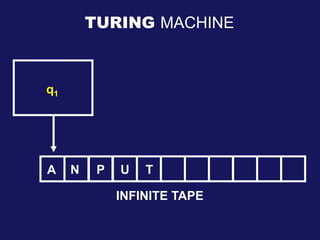
2. It then describes Turing machines, including their components, configurations, and definitions of Turing-recognizable and decidable languages. Examples of Turing machines are provided.
3. Finally, it discusses the Church-Turing thesis, encoding computational models as strings, and the decidability of problems about finite automata, context-free grammars, and Turing machines. The document appears to be lecture slides on formal languages and computability.