Turing Machine presentation for college level presentation in easy way,

1. Topic:- Turing Machine
Presented by
Sayan Das
University Roll No.: 11000123035
5th
Semester
Subject: Theory of Computation Code: PEC-IT501A
Faculty’s Name: Mr. Prasanta Mandal
Government College of Engineering &
Textile Technology, Serampore
Department of Computer Science and Engineering

2. Outline
1.Introduction
2.Mathematically Representation of Turing Machine
3.Working Principle
4.Types of Turing Machines
5.Example Problem
6.Importance of Turing Machines in TOC
7.Advantages & Limitations
8.Modern Implications and Applications
9.Conclusion
10.References

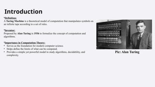
3. Introduction
•Definition:
A Turing Machine is a theoretical model of computation that manipulates symbols on
an infinite tape according to a set of rules.
•Inventor:
Proposed by Alan Turing in 1936 to formalize the concept of computation and
algorithms.
•Importance in Computation Theory:
• Serves as the foundation for modern computer science.
• Helps define the limits of what can be computed.
• Provides a simple yet powerful model to study algorithms, decidability, and
complexity.
Pic: Alan Turing

4. Mathematically Representation of Turing Machine
A Turing Machine is mathematically represented as: M = (Q, Σ, Γ, δ, q0, B, F)
Brief meaning of each part:
1. Q – Finite set of states (e.g., {q , q , q , …}).
₀ ₁ ₂
2. Σ (Sigma) – Input alphabet (symbols allowed in the input, excluding blank).
3. Γ (Gamma) – Tape alphabet (includes Σ plus blank symbol and possibly extra symbols).
␣
4. δ (Delta) – Transition function:
δ:Q×Γ→Q×Γ×{L,R}
Decides the next state, what symbol to write, and which direction to move (Left or Right).
6. q₀ – Start state (initial state when computation begins).
7. B -- the blank symbol. This symbol is in Γ but not in Σ.
8. F -- the set of final or accepting states, a subset of Q.

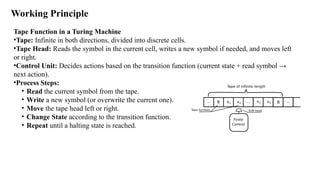
5. Tape Function in a Turing Machine
•Tape: Infinite in both directions, divided into discrete cells.
•Tape Head: Reads the symbol in the current cell, writes a new symbol if needed, and moves left
or right.
•Control Unit: Decides actions based on the transition function (current state + read symbol →
next action).
•Process Steps:
• Read the current symbol from the tape.
• Write a new symbol (or overwrite the current one).
• Move the tape head left or right.
• Change State according to the transition function.
• Repeat until a halting state is reached.
Working Principle

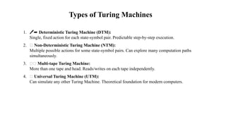
6. Types of Turing Machines
1. ️
➡️
🖊️ Deterministic Turing Machine (DTM):
Single, fixed action for each state-symbol pair. Predictable step-by-step execution.
2. 🔀 Non-Deterministic Turing Machine (NTM):
Multiple possible actions for some state-symbol pairs. Can explore many computation paths
simultaneously.
3. 📜📜 Multi-tape Turing Machine:
More than one tape and head. Reads/writes on each tape independently.
4. 🌐 Universal Turing Machine (UTM):
Can simulate any other Turing Machine. Theoretical foundation for modern computers.

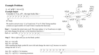
7. Example Problem:
L ={ an
bn
| n>=1}
Example Input:
Consider n=3 so, a3
b3
, the tape looks like −
B= blank
We need to convert every ‘a’ as X and every ‘b’ as Y. If the Turing machine
contains an equal number of X and Y then it reaches the final state.
Step 1 − Consider the initial state as q0. This state replace ‘a’ as X and move to right,
now state changes for q0 toq1, so the transition function is −
δ(q0, a) = (q1,X,R)
Step 2 − Move right until you see the blank symbol.
δ(q1, a) = (q1,a,R)
δ(q1, b) = (q1,b,R)
After reaching the blank symbol B, move left and change the state to q2, because we need to
change the last ‘b’ to Y.
δ(q1, B) = (q2,B,L) //1st iteration
δ(q1, Y) = (q2,Y,L) // remaining iterations

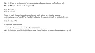
8. Step 3 − When we see the symbol ‘b’, replace it as Y and change the state to q3 and move left.
δ(q2, B) = (q3,Y,L)
Step 4 − Move to left until reach the symbol X.
δ(q3, a) = (q3,a,L)
δ(q3, b) = (q3,b,L)
When we reach X move right and change the state as q0, and the next iteration is started.
After replacing every ‘a’ and ‘b’ as X and Y by changing the states to q0 to q4, we get the following −
δ(q0, Y) = (q4,Y,N)
N represents No movement.
q4 is the final state and q0 is the initial state of the Turing Machine, the intermediate states are q1, q2, q3.

9. Importance of Turing Machines in TOC
1.Decidability & Undecidability
1.Decidability: Problems for which a Turing Machine can produce a yes/no answer in a finite
amount of time.
2.Undecidability: Problems for which no Turing Machine can provide a guaranteed solution
(e.g., Halting Problem).
2.Church–Turing Thesis
1.States that any computation that can be performed by an algorithm can be performed by a
Turing Machine.
2.Equates the intuitive notion of "computable" with "Turing-computable."
3.Foundation of Computer Science
1.Provides a universal model for defining computation.
2.Forms the basis for programming languages, algorithm analysis, and complexity theory.
3.Helps classify problems into solvable, unsolvable, and computationally hard.

10. Advantages & Limitations
Advantages:
•Simple yet powerful: The concept of a Turing Machine is easy to understand but
capable of solving complex problems.
•Universality: Can simulate any algorithm, making it the theoretical foundation of
computing.
Limitations:
•Infinite tape assumption: Real-world computers have finite memory, unlike the
theoretical model.
•Undecidable problems: Some problems cannot be solved by any Turing Machine
(e.g., Halting Problem).

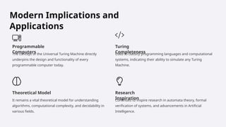
11. Modern Implications and
Applications
Programmable
Computers
The concept of the Universal Turing Machine directly
underpins the design and functionality of every
programmable computer today.
Turing
Completeness
Used to classify programming languages and computational
systems, indicating their ability to simulate any Turing
Machine.
Theoretical Model
It remains a vital theoretical model for understanding
algorithms, computational complexity, and decidability in
various fields.
Research
Inspiration
Continues to inspire research in automata theory, formal
verification of systems, and advancements in Artificial
Intelligence.

12. Conclusion: The Legacy of the Turing Machine
The Turing Machine, while abstract, is an incredibly powerful model of computation. It fundamentally defines what can and cannot be
computed algorithmically, providing an enduring framework for computational theory.
Alan Turing’s pioneering work continues to influence and shape computer science, mathematics, and logic, nearly 90 years after its inception,
remaining as foundational as ever.
References:
•Michael Sipser, Introduction to the Theory of Computation, 3rd Edition, Cengage Learning, 2012.
•Hopcroft, J.E., Motwani, R., Ullman, J.D., Introduction to Automata Theory, Languages, and Computation, 3rd Edition, Pearson, 2006.
•Alan M. Turing, “On Computable Numbers, with an Application to the Entscheidungsproblem,” Proceedings of the London Mathematical
Society, 1936.
•Online resource: GeeksforGeeks – Turing Machine
•Online resource: Wikipedia – Turing Machine

13. THANK YOU