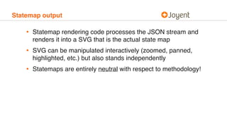
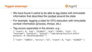
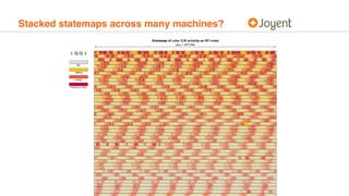
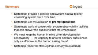
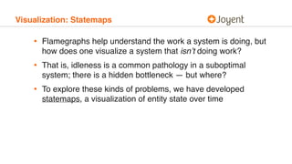
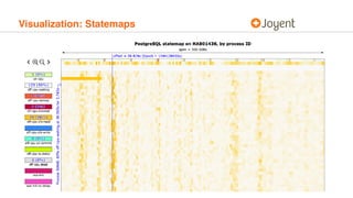
Visualizing Systems with Statemaps
CTO
bryan@joyent.com
Bryan Cantrill
@bcantrill
The stack of abstraction
• Our software systems are built as stacks of abstraction
• These stacks allow us to stand on the shoulders of history — to
reuse components without rebuilding them
• We can do this because of the software paradox: software is
both information and machine, exhibiting properties of both
• Our stacks are higher and run deeper than we can see or know:
software is opaque; the nature of abstraction is to seal us from
what runs beneath!
Run silent, run deep
• Not only is the stack deep, it is silent
• Running software emits neither light nor heat; it makes no
sound; it attracts no mass; it (mostly) has no odor
• Running software is — by all conventional notions — unseeable
• This generally isn’t a bad thing, as long as it all works…
Hurricanes from butterflies
• When the stack of abstraction performs pathologically, its power
transmogrifies to peril: layering amplifies performance
pathologies but hinders insight
• Work amplifies as we go down the stack
• Latency amplifies as we go up the stack
• Seemingly minor issues in one layer can cascade into systemic
pathological performance…
• As the system becomes dominated by its outliers, butterflies
spawn hurricanes of pathological performance
Debugging the hurricanes
• Understanding a pathologically performing system is
excruciatingly difficult:
• Symptoms are often far removed from root cause
• There may not be a single root cause but several
• The system is dynamic and may change without warning
• Improvements to the system are hard to model and verify
• Emphatically, this is not “tuning” — it is debugging
How do we debug?
• To debug methodically, we must resist the temptation to quick
hypotheses, focusing rather on questions and observations
• Iterating between questions and observations gathers the facts
that will constrain future hypotheses
• These facts can be used to disconfirm hypotheses!
• How do we ask questions?
• How do we make observations?
Asking questions
• For performance debugging, the initial question formulation is
particularly challenging: where does one start?
• Resource-centric methodologies like the USE Method
(Utilization/Saturation/Errors) can be excellent starting points…
• But keep these methodologies in their context: they provide
initial questions to ask — they are not recipes for debugging
arbitrary performance pathologies!
Making observations
• Questions are answered through observation
• But — reminder! — software cannot by conventionally seen!
• It is up to the system itself to have the capacity to be seen
• This capacity is the system’s observability — and without it, we
are reduced to guessing
• Do not conflate software observability with control theory’s
definition of observability!
• Software is observable when it can answer your question about
its behavior — software observability is not a boolean!
The pillars of observability
• Much has been made of the so-called “pillars of observability”:
monitoring, logging and instrumentation
• Each of these is important, for each has within it the capacity to
answer questions about the system
• But each also has limitations!
• Their shared limitation: each can only be as effective as the
observer — they cannot answer questions not asked!
• Observability seeks to answer questions asked and prompt new
ones: the human is the foundation of observability!
Observability through instrumentation
• Static instrumentation modifies source to provide semantically
relevant information, e.g., via logging or counters
• Dynamic instrumentation allows for the system to be changed
while running to emit data, e.g. DTrace, OpenTracing
• Both mechanisms of instrumentation are essential!
• Static instrumentation provides the observations necessary for
early question formulation…
• Dynamic instrumentation answers deeper, ad hoc questions
Aggregation
• When instrumenting the system, it can become overwhelmed
with the overhead of instrumentation
• Aggregation is essential for scalable, non-invasive
instrumentation — and is a first-class primitive in (e.g.) DTrace
• But aggregation also eliminates important dimensions of data,
especially with respect to time; some questions may only be
answered with disaggregated data!
• Use aggregation for performance debugging — but also
understand its limits!
Visualization
• The visual cortex is unparalleled at detecting patterns
• The value of visualizing data is not merely providing answers,
but also (and especially) provoking new questions
• Our systems are so large, complicated and abstract that there is
not one way to visualize them, but many
• The visualization of systems and their representations is an
essential facet of system observability!
Visualization: Gnuplot
• Graphs are terrific — so much so that we should not restrict
ourselves to the captive graphs found in bundled software!
• An ad hoc plotting tool is essential for performance debugging;
and Gnuplot is an excellent (if idiosyncratic) one
• Gnuplot is easily combined with workhorses like awk or perl
• That Gnuplot is an essential tool helps to set expectation
around performance debugging tools: they are not magicians!
Visualization: Heatmaps
Visualization: Flamegraphs
Visualization: Statemaps
• Flamegraphs help understand the work a system is doing, but
how does one visualize a system that isn’t doing work?
• That is, idleness is a common pathology in a suboptimal
system; there is a hidden bottleneck — but where?
• To explore these kinds of problems, we have developed
statemaps, a visualization of entity state over time
Visualization: Statemaps
Statemap input data
• Statemaps operate on a payload of concatenated JSON where
each line corresponds to a state transition for an entity:


{ "time": "52524411", "entity": "30080", "state": 0 }

{ "time": "52587486", "entity": "30137", "state": 0 }
{ "time": "52769425", "entity": "30080", "state": 4 }
{ "time": "52895402", "entity": "30137", "state": 1 }
{ "time": "53177670", "entity": "62308", "state": 0 }
{ "time": "53230742", "entity": "30137", "state": 0 }
{ "time": "53268043", "entity": "30137", "state": 1 }
{ "time": "53562441", "entity": "62308", "state": 4 }
{ "time": "53616633", "entity": "30137", "state": 0 }
{ "time": "53762283", "entity": "30137", "state": 6 }

…
Statemap input data
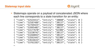
• States are described in JSON metadata header, e.g.:


{

"start": [ 1544138397, 322335287 ],

"title": "PostgreSQL statemap on HAB01436, by process ID",

"host": "HAB01436",

"entityKind": "Process",

"states": {

"on-cpu": {"value": 0, "color": "#DAF7A6" },

"off-cpu-waiting": {"value": 1, "color": "#f9f9f9" },

"off-cpu-semop": {"value": 2, "color": "#FF5733" },

"off-cpu-blocked": {"value": 3, "color": "#C70039" },

"off-cpu-zfs-read": {"value": 4, "color": "#FFC300" },

"off-cpu-zfs-write": {"value": 5, "color": "#338AFF" },

"off-cpu-zil-commit": {"value": 6, "color": "#66FFCC" },

"off-cpu-tx-delay": {"value": 7, "color": "#CCFF00" },

"off-cpu-dead": {"value": 8, "color": "#E0E0E0" },

"wal-init": {"value": 9, "color": "#dd1871" },

"wal-init-tx-delay": {"value": 10, "color": "#fd4bc9" }

}

}
Statemap output
• Statemap rendering code processes the JSON stream and
renders it into a SVG that is the actual state map
• SVG can be manipulated interactively (zoomed, panned,
highlighted, etc.) but also stands independently
• Statemaps are entirely neutral with respect to methodology!
Instrumentation for statemaps
• Statemaps themselves — like gnuplot — are entirely generic to
input data: they visualize arbitrary state over arbitrary time
• We have developed example statemap-generating dynamic
instrumentation for database, CPU, I/O, filesystem operations
• The data rate in terms of state transitions per second varies
based on what is being instrumented: from <10/sec to >1M/sec
Coalescing states
• For even modestly large inputs, adjacent states must be
coalesced to allow for reasonable visualization
• When this aggregation is required, the statemap rendering code
coalesces the least significant two adjacent states — allowing
for larger trends to stay intact
• The threshold at which states are coalesced can be dynamically
adjusted to allow for higher resolution
• Importantly, the original data retains all state transitions!
Coalescing states
Coalescing states
Tagged statemaps
• We have found it useful to be able to tag states with immutable
information that describes the context around the state
• For example, tagging a state for CPU execution with immutable
context information (process, thread, etc.)
• Tag occurs separately in the stream, e.g.:


{ "state": 0, "tag": "d136827", "pid": "51943", "tid": "1",
"execname": "postgres", "psargs": "/opt/postgresql/9.6.3/bin/
postgres -D /manatee/pg/data" }

…

{ "time": "330931", "entity": "12", "state": 0, "tag": "d136827" }
Tagged statemaps
Stacked statemaps
• We have found it useful to be able to stack statemaps from
either disjoint sources or disjoint machines
• Allows for activity in one domain or machine to be tightly
correlated with activity in another domain or machine
• Across machines, can be subject to wall clock skew…
• …but if wall clocks are skewing within the datacenter, there are
likely bigger problems!
Stacked statemaps across domains
Stacked statemaps across machines
Stacked statemaps across many machines?
Statemaps
• Statemaps provide a generic and system-neutral tool for
visualizing system state over time
• Statemaps use visualization to prompt questions
• Statemaps work in concert with system observability facilities
that can answer the questions that statemaps raise
• We must keep the human in mind when developing for
observability — the capacity to answer arbitrary questions is
only as effective as the human asking them!
• Statemap renderer: https://github.com/joyent/statemap

Visualizing Systems with Statemaps

  • 1.
    Visualizing Systems withStatemaps CTO bryan@joyent.com Bryan Cantrill @bcantrill
  • 2.
    The stack ofabstraction • Our software systems are built as stacks of abstraction • These stacks allow us to stand on the shoulders of history — to reuse components without rebuilding them • We can do this because of the software paradox: software is both information and machine, exhibiting properties of both • Our stacks are higher and run deeper than we can see or know: software is opaque; the nature of abstraction is to seal us from what runs beneath!
  • 3.
    Run silent, rundeep • Not only is the stack deep, it is silent • Running software emits neither light nor heat; it makes no sound; it attracts no mass; it (mostly) has no odor • Running software is — by all conventional notions — unseeable • This generally isn’t a bad thing, as long as it all works…
  • 4.
    Hurricanes from butterflies •When the stack of abstraction performs pathologically, its power transmogrifies to peril: layering amplifies performance pathologies but hinders insight • Work amplifies as we go down the stack • Latency amplifies as we go up the stack • Seemingly minor issues in one layer can cascade into systemic pathological performance… • As the system becomes dominated by its outliers, butterflies spawn hurricanes of pathological performance
  • 5.
    Debugging the hurricanes •Understanding a pathologically performing system is excruciatingly difficult: • Symptoms are often far removed from root cause • There may not be a single root cause but several • The system is dynamic and may change without warning • Improvements to the system are hard to model and verify • Emphatically, this is not “tuning” — it is debugging
  • 6.
    How do wedebug? • To debug methodically, we must resist the temptation to quick hypotheses, focusing rather on questions and observations • Iterating between questions and observations gathers the facts that will constrain future hypotheses • These facts can be used to disconfirm hypotheses! • How do we ask questions? • How do we make observations?
  • 7.
    Asking questions • Forperformance debugging, the initial question formulation is particularly challenging: where does one start? • Resource-centric methodologies like the USE Method (Utilization/Saturation/Errors) can be excellent starting points… • But keep these methodologies in their context: they provide initial questions to ask — they are not recipes for debugging arbitrary performance pathologies!
  • 8.
    Making observations • Questionsare answered through observation • But — reminder! — software cannot by conventionally seen! • It is up to the system itself to have the capacity to be seen • This capacity is the system’s observability — and without it, we are reduced to guessing • Do not conflate software observability with control theory’s definition of observability! • Software is observable when it can answer your question about its behavior — software observability is not a boolean!
  • 9.
    The pillars ofobservability • Much has been made of the so-called “pillars of observability”: monitoring, logging and instrumentation • Each of these is important, for each has within it the capacity to answer questions about the system • But each also has limitations! • Their shared limitation: each can only be as effective as the observer — they cannot answer questions not asked! • Observability seeks to answer questions asked and prompt new ones: the human is the foundation of observability!
  • 10.
    Observability through instrumentation •Static instrumentation modifies source to provide semantically relevant information, e.g., via logging or counters • Dynamic instrumentation allows for the system to be changed while running to emit data, e.g. DTrace, OpenTracing • Both mechanisms of instrumentation are essential! • Static instrumentation provides the observations necessary for early question formulation… • Dynamic instrumentation answers deeper, ad hoc questions
  • 11.
    Aggregation • When instrumentingthe system, it can become overwhelmed with the overhead of instrumentation • Aggregation is essential for scalable, non-invasive instrumentation — and is a first-class primitive in (e.g.) DTrace • But aggregation also eliminates important dimensions of data, especially with respect to time; some questions may only be answered with disaggregated data! • Use aggregation for performance debugging — but also understand its limits!
  • 12.
    Visualization • The visualcortex is unparalleled at detecting patterns • The value of visualizing data is not merely providing answers, but also (and especially) provoking new questions • Our systems are so large, complicated and abstract that there is not one way to visualize them, but many • The visualization of systems and their representations is an essential facet of system observability!
  • 13.
    Visualization: Gnuplot • Graphsare terrific — so much so that we should not restrict ourselves to the captive graphs found in bundled software! • An ad hoc plotting tool is essential for performance debugging; and Gnuplot is an excellent (if idiosyncratic) one • Gnuplot is easily combined with workhorses like awk or perl • That Gnuplot is an essential tool helps to set expectation around performance debugging tools: they are not magicians!
  • 14.
  • 15.
  • 16.
    Visualization: Statemaps • Flamegraphshelp understand the work a system is doing, but how does one visualize a system that isn’t doing work? • That is, idleness is a common pathology in a suboptimal system; there is a hidden bottleneck — but where? • To explore these kinds of problems, we have developed statemaps, a visualization of entity state over time
  • 17.
  • 18.
    Statemap input data •Statemaps operate on a payload of concatenated JSON where each line corresponds to a state transition for an entity:
 
 { "time": "52524411", "entity": "30080", "state": 0 }
 { "time": "52587486", "entity": "30137", "state": 0 } { "time": "52769425", "entity": "30080", "state": 4 } { "time": "52895402", "entity": "30137", "state": 1 } { "time": "53177670", "entity": "62308", "state": 0 } { "time": "53230742", "entity": "30137", "state": 0 } { "time": "53268043", "entity": "30137", "state": 1 } { "time": "53562441", "entity": "62308", "state": 4 } { "time": "53616633", "entity": "30137", "state": 0 } { "time": "53762283", "entity": "30137", "state": 6 }
 …
  • 19.
    Statemap input data •States are described in JSON metadata header, e.g.:
 
 
 {
 "start": [ 1544138397, 322335287 ],
 "title": "PostgreSQL statemap on HAB01436, by process ID",
 "host": "HAB01436",
 "entityKind": "Process",
 "states": {
 "on-cpu": {"value": 0, "color": "#DAF7A6" },
 "off-cpu-waiting": {"value": 1, "color": "#f9f9f9" },
 "off-cpu-semop": {"value": 2, "color": "#FF5733" },
 "off-cpu-blocked": {"value": 3, "color": "#C70039" },
 "off-cpu-zfs-read": {"value": 4, "color": "#FFC300" },
 "off-cpu-zfs-write": {"value": 5, "color": "#338AFF" },
 "off-cpu-zil-commit": {"value": 6, "color": "#66FFCC" },
 "off-cpu-tx-delay": {"value": 7, "color": "#CCFF00" },
 "off-cpu-dead": {"value": 8, "color": "#E0E0E0" },
 "wal-init": {"value": 9, "color": "#dd1871" },
 "wal-init-tx-delay": {"value": 10, "color": "#fd4bc9" }
 }
 }
  • 20.
    Statemap output • Statemaprendering code processes the JSON stream and renders it into a SVG that is the actual state map • SVG can be manipulated interactively (zoomed, panned, highlighted, etc.) but also stands independently • Statemaps are entirely neutral with respect to methodology!
  • 21.
    Instrumentation for statemaps •Statemaps themselves — like gnuplot — are entirely generic to input data: they visualize arbitrary state over arbitrary time • We have developed example statemap-generating dynamic instrumentation for database, CPU, I/O, filesystem operations • The data rate in terms of state transitions per second varies based on what is being instrumented: from <10/sec to >1M/sec
  • 22.
    Coalescing states • Foreven modestly large inputs, adjacent states must be coalesced to allow for reasonable visualization • When this aggregation is required, the statemap rendering code coalesces the least significant two adjacent states — allowing for larger trends to stay intact • The threshold at which states are coalesced can be dynamically adjusted to allow for higher resolution • Importantly, the original data retains all state transitions!
  • 23.
  • 24.
  • 25.
    Tagged statemaps • Wehave found it useful to be able to tag states with immutable information that describes the context around the state • For example, tagging a state for CPU execution with immutable context information (process, thread, etc.) • Tag occurs separately in the stream, e.g.:
 
 { "state": 0, "tag": "d136827", "pid": "51943", "tid": "1", "execname": "postgres", "psargs": "/opt/postgresql/9.6.3/bin/ postgres -D /manatee/pg/data" }
 …
 { "time": "330931", "entity": "12", "state": 0, "tag": "d136827" }
  • 26.
  • 27.
    Stacked statemaps • Wehave found it useful to be able to stack statemaps from either disjoint sources or disjoint machines • Allows for activity in one domain or machine to be tightly correlated with activity in another domain or machine • Across machines, can be subject to wall clock skew… • …but if wall clocks are skewing within the datacenter, there are likely bigger problems!
  • 28.
  • 29.
  • 30.
  • 31.
    Statemaps • Statemaps providea generic and system-neutral tool for visualizing system state over time • Statemaps use visualization to prompt questions • Statemaps work in concert with system observability facilities that can answer the questions that statemaps raise • We must keep the human in mind when developing for observability — the capacity to answer arbitrary questions is only as effective as the human asking them! • Statemap renderer: https://github.com/joyent/statemap