This document presents a sample assignment from matlabhomeworkhelper.com that explains advanced mathematical concepts in complex analysis using MATLAB. It focuses on Cauchy's integral formula and includes practical examples of numerical integration, contour visualization, and symbolic computation. The assignment enhances understanding of both theoretical and practical aspects of solving complex integrals.

1. Title: Visualizing and Solving Complex Integrals with
MATLAB Tools
Visit: www.matlabhomeworkhelper.com
Email: support@matlabhomeworkhelper.com
Phone: +1 (315)-557-6473

2. Introduction
This sample assignment from
MATLABHomeworkHelper.com simplifies advanced
mathematical concepts through practical programming
applications. It delves into complex analysis techniques,
focusing on Cauchy's integral formula to evaluate integrals
over specific contours in the complex plane. Utilizing
MATLAB, you’ll numerically integrate complex functions,
visualize contours, and apply symbolic computation to
handle singularities and validate formulas. This example
enhances your understanding of how MATLAB can
efficiently solve complex analysis problems, ensuring a
well-rounded grasp of both theoretical and practical
aspects.

3. Problem 1

4. Solution
a)

5. Solution
a)

6. Solution
b)

7. Solution
c)

8. Solution
c)

9. Solution
d)

10. Solution
d)

11. Solution
MATLAB code for part (a):
syms z
f = sin(pi*z^2) + cos(pi*z^2);
integrand = f / ((z - 1) * (z - 2));
residue_at_1 = subs(f, z, 1) / (1 - 2);
residue_at_2 = subs(f, z, 2) / (2 - 1);
integral_value = 2 * pi * 1i * (residue_at_1
+ residue_at_2);
disp(vpa(integral_value));

12. Solution
MATLAB code for part (b):
syms z
f = (z^2 + 1) / z^2;
% Calculate residue at z = 0 (pole of order
2)
residue = limit(diff(f * z^2, z, 1) /
factorial(1), z, 0);
integral_value = 2 * pi * 1i * residue;
disp(vpa(integral_value));

13. Solution
MATLAB code for part (c):
syms z
f = z^2;
integrand = f / (z - 1);
residue_at_1 = subs(f, z, 1);
integral_value = 2 * pi * 1i * residue_at_1;
disp(vpa(integral_value));

14. Solution
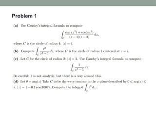
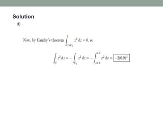
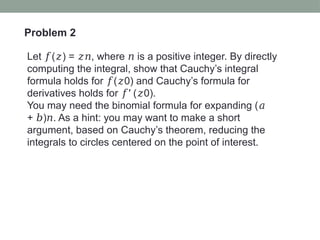
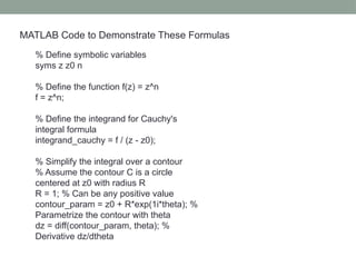
MATLAB code for part (d):
% Define the function z(t) along the contour
z_contour = @(theta) (1 - 0.1 * cos(100 *
theta)) .* exp(1i * theta);
% Define the integrand z^2 dz/dtheta (dz/dtheta
is needed for the line integral)
integrand = @(theta) z_contour(theta).^2 .* (1i *
(1 - 0.1 * cos(100 * theta)) .* exp(1i * theta) ...
- 10 * sin(100 * theta) .* exp(1i * theta));
% Perform the numerical integration over the
interval [0, pi]
integral_value = integral(@(theta)
integrand(theta), 0, pi, 'ArrayValued', true);
disp('Numerical value of the integral:');
disp(vpa(integral_value, 8));

15. Problem 2
Let ( ) = , where is a positive integer. By directly
𝑓 𝑧 𝑧𝑛 𝑛
computing the integral, show that Cauchy’s integral
formula holds for ( 0) and Cauchy’s formula for
𝑓 𝑧
derivatives holds for ′ ( 0).
𝑓 𝑧
You may need the binomial formula for expanding (𝑎
+ ) . As a hint: you may want to make a short
𝑏 𝑛
argument, based on Cauchy’s theorem, reducing the
integrals to circles centered on the point of interest.

16. Solution

17. Solution

18. Solution

19. MATLAB Code to Demonstrate These Formulas
% Define symbolic variables
syms z z0 n
% Define the function f(z) = z^n
f = z^n;
% Define the integrand for Cauchy's
integral formula
integrand_cauchy = f / (z - z0);
% Simplify the integral over a contour
% Assume the contour C is a circle
centered at z0 with radius R
R = 1; % Can be any positive value
contour_param = z0 + R*exp(1i*theta); %
Parametrize the contour with theta
dz = diff(contour_param, theta); %
Derivative dz/dtheta

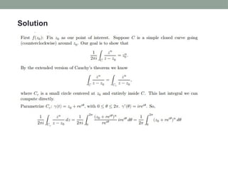
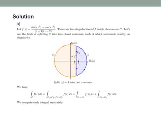
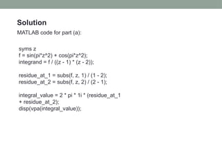
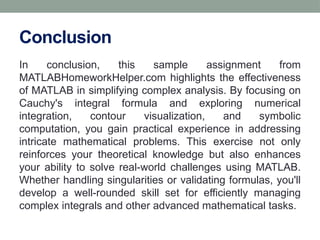
20. % Substitute the parametrization into the
integrand
integrand_param = subs(integrand_cauchy,
z, contour_param) * dz;
% Integrate with respect to theta over [0,
2*pi]
cauchy_integral = int(integrand_param,
theta, 0, 2*pi);
% Simplify the result and divide by (2*pi*i)
f_z0 = simplify(cauchy_integral / (2*pi*1i));
% Display the result
disp('Cauchy Integral Formula Result for
f(z) = z^n:');
disp(f_z0);
% Now, calculate the derivative of f(z) =
z^n
f_derivative = diff(f, z);

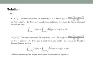
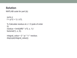
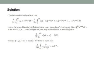
21. % Define the integrand for the derivative
formula
integrand_derivative = f_derivative / (z - z0);
% Substitute the parametrization into the
integrand
integrand_param_derivative =
subs(integrand_derivative, z, contour_param)
* dz;
% Integrate with respect to theta over [0, 2*pi]
cauchy_derivative_integral =
int(integrand_param_derivative, theta, 0,
2*pi);
% Simplify the result and divide by (2*pi*i)
f_prime_z0 =
simplify(cauchy_derivative_integral /
(2*pi*1i));
% Display the result
disp('Cauchy Integral Formula Result for f''(z)
= n*z^{n-1}:');

22. Conclusion
In conclusion, this sample assignment from
MATLABHomeworkHelper.com highlights the effectiveness
of MATLAB in simplifying complex analysis. By focusing on
Cauchy's integral formula and exploring numerical
integration, contour visualization, and symbolic
computation, you gain practical experience in addressing
intricate mathematical problems. This exercise not only
reinforces your theoretical knowledge but also enhances
your ability to solve real-world challenges using MATLAB.
Whether handling singularities or validating formulas, you'll
develop a well-rounded skill set for efficiently managing
complex integrals and other advanced mathematical tasks.