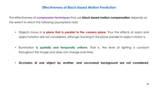
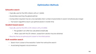
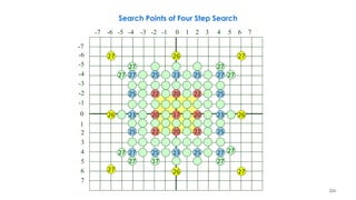
Download as PDF, PPTX


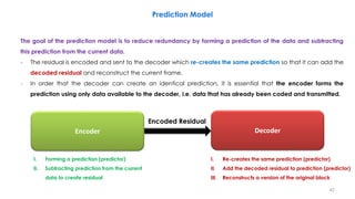
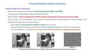
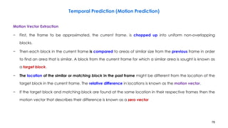
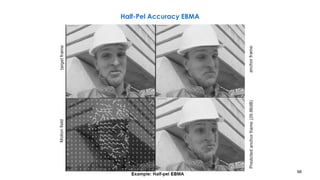
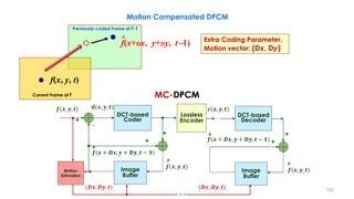
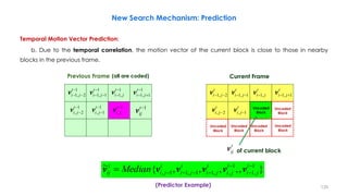
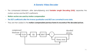
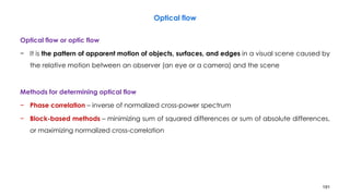
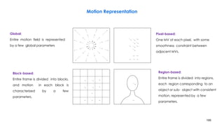
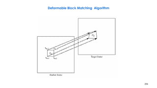
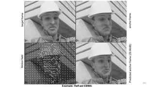
 Frame 2 s[x,y,t](current) Partition of frame 2 into blocks (schematic)
Frame 2 with displacement vectors Difference between motion-compensated
prediction and current frame u[x,y,t] Referenced blocks in frame 1
Block-based Motion Estimation and Compensation, Ex3](https://image.slidesharecdn.com/videocompressionpart2section2videocodingconceptsbymr-200411173523/85/Video-Compression-Part-2-Section-2-Video-Coding-Concepts-82-320.jpg)
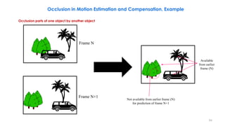


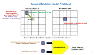
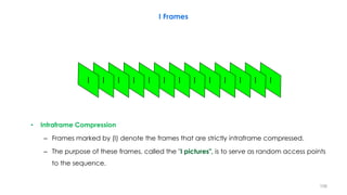
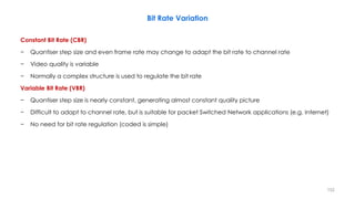
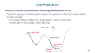
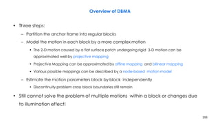
![Macro-block
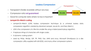
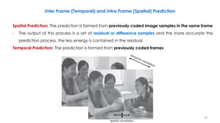
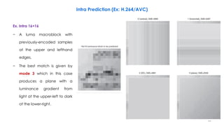
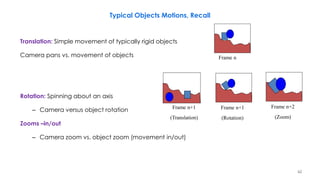
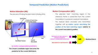
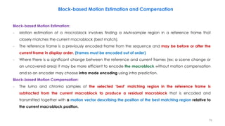
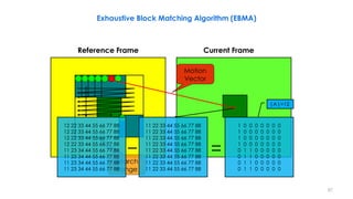
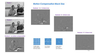
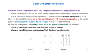
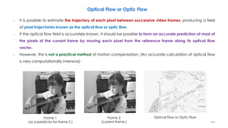
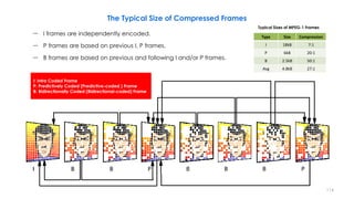
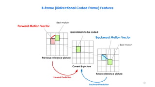
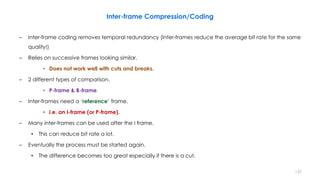
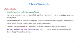
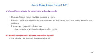
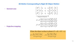
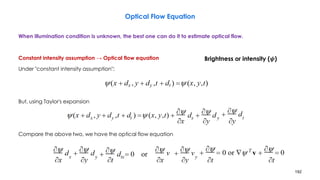
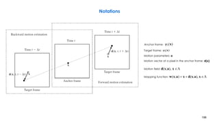
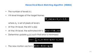
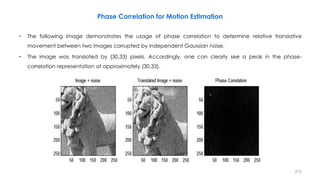
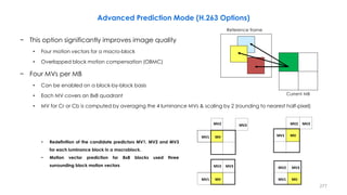
– Motion estimation of a macroblock involves finding a 16×16-sample
region in a reference frame that closely matches the current
macroblock.
– Luminance: 16x16, four 8x8 blocks
– Chrominance: two 8x8 blocks
– Motion estimation only performed for luminance component
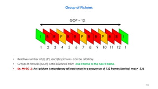
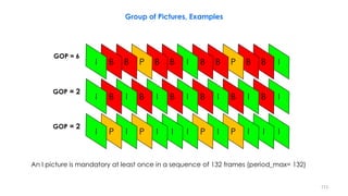
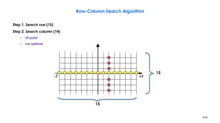
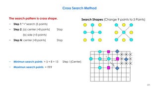
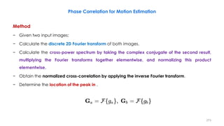
Motion Vector Range
– [ -15, 15]
– MB: 16 x 16
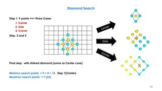
15
15
15 15
Search Area in Reference Frame
MB
105
Ex: Motion Estimation in H.261
𝑪𝒓 𝑪𝒃
𝒀
𝒀 𝟎 𝒀 𝟏
𝒀 𝟐 𝒀 𝟑](https://image.slidesharecdn.com/videocompressionpart2section2videocodingconceptsbymr-200411173523/85/Video-Compression-Part-2-Section-2-Video-Coding-Concepts-105-320.jpg)
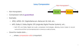
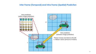
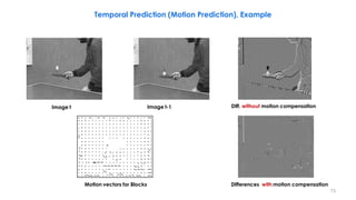
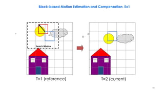
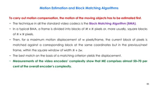
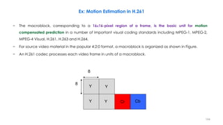
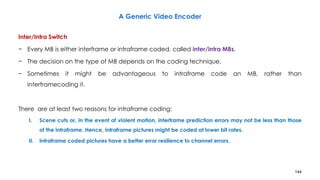
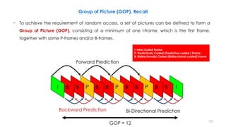
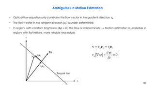
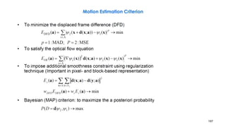
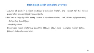
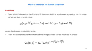
![− Integer pixel ME search only
− Motion vectors are differentially & separately encoded
− 11-bit VLC for MVD (Motion Vector Delta)
Example
MV = 2 2 3 5 3 1 -1
MVD = 0 1 2 -2 -2 -2…
− Binary: 1 010 0010 0011 0011 0011…
]1[][
]1[][
nMVnMVMVD
nMVnMVMVD
yyy
xxx
106
MVD VLC
… …
-2 & 30 0011
-1 011
0 1
1 010
2 & -30 0010
3 & -29 0001 0
Ex: Motion Vectors Coding in H.261
𝐌𝐕𝐃 = 𝒇(𝒙, 𝒚, 𝒕) − 𝒇(𝒙+𝜟𝒙, 𝒚 + 𝜟𝒚, 𝒕 − 𝟏)](https://image.slidesharecdn.com/videocompressionpart2section2videocodingconceptsbymr-200411173523/85/Video-Compression-Part-2-Section-2-Video-Coding-Concepts-106-320.jpg)
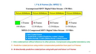
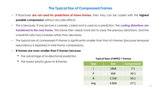
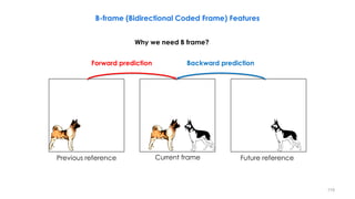
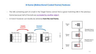
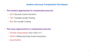
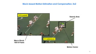
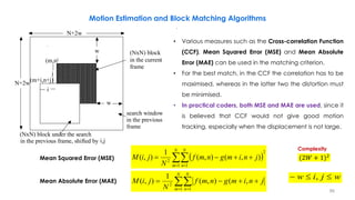
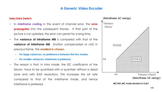
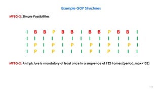
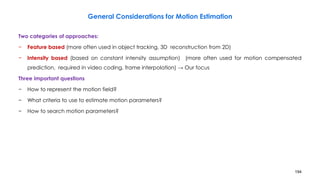
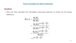
![- [ + ] =
Past reference Target Future reference
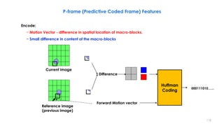
Encode:
− Two motion vectors - difference in spatial location of macro-blocks.
• Two motion vectors are estimated (one to a past frame, one to a future frame).
− Small difference in content of the macro-blocks
126
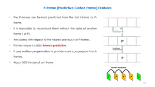
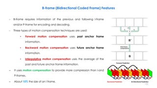
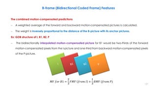
Interpolative compensation uses the waited average of the past and future anchor frame information.
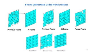
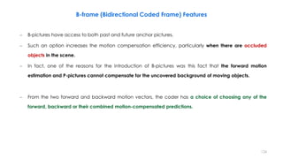
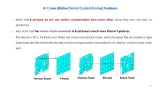
B-frame (Bidirectional Coded Frame) Features
FMV
BMV
𝒘 𝟏 𝒘 𝟐
DCT + Quant + RLE
Huffman CodeMotion Vectors 000111010…...](https://image.slidesharecdn.com/videocompressionpart2section2videocodingconceptsbymr-200411173523/85/Video-Compression-Part-2-Section-2-Video-Coding-Concepts-126-320.jpg)

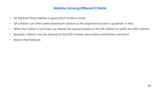
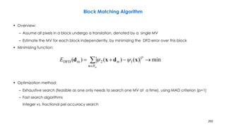
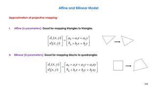
![143
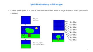
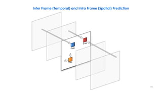
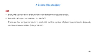
BD –Block Difference
DBD – Displaced Block Difference
X
X
3
2.7
MC
No MC
256
DBD
y
x
256
BD
1.5
0.5
1
DBD c[x, y] r[x dx, y dy]
256 MB
1
BD c[x, y] r[x, y]
256 MB
1
𝑦 = 𝑥/1.1
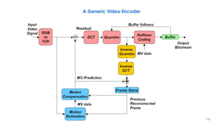
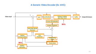
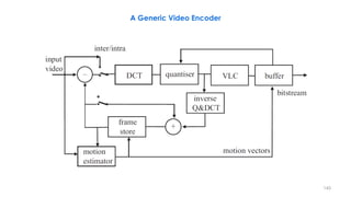
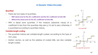
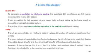
A Generic Video Encoder
– Not all blocks are motion compensated
– The one which generates less bits are preferred.
Motion Compensation Decision Characteristic (H.261)](https://image.slidesharecdn.com/videocompressionpart2section2videocodingconceptsbymr-200411173523/85/Video-Compression-Part-2-Section-2-Video-Coding-Concepts-143-320.jpg)

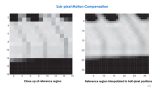
![210
(x, y) (x+1,y)
(x,y +1) (x+1 ,y+1)
(2x +1,2y)
(2x,2y +1) (2x +1,2y+1)
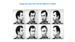
Bilinear Interpolation
O[2x,2y]=I[x,y]
O[2x+1,2y]=(I[x,y]+I[x+1,y])/2
O[2x,2y+1]=(I[x,y]+I[x+1,y])/2
O[2x+1,2y+1]=(I[x,y]+I[x+1,y]+I[x,y+1]+I[x+1,y+1])/4
(2x, 2y)](https://image.slidesharecdn.com/videocompressionpart2section2videocodingconceptsbymr-200411173523/85/Video-Compression-Part-2-Section-2-Video-Coding-Concepts-210-320.jpg)

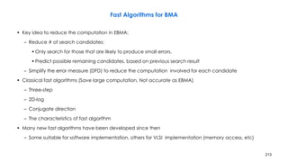

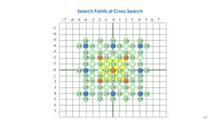
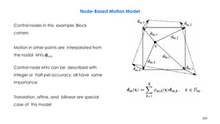
![218
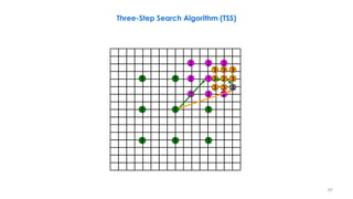
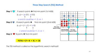
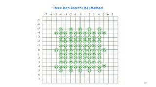
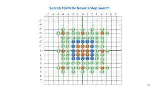
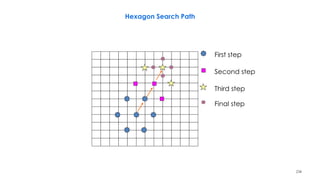
Three-Step Search Algorithm Example
2
3 3 3
3 2 3 2
1 1 2 3 3 3 2
1
2 2 2
1 1
1
1 1 1
n denotes a search point of step n
i 6 i 5 i 4 i 3 i 2 i 1 i i 1 i 2 i 3 i 4 i 5 i 6 j 6
j 5
j 4
j 3
j 2
j 1
j
j 1
j 2
j 3
j 4
j 5
j 6
The best matching MVs in steps 1–3 are (3,3), (3,5),
and (2,6). The final MV is (2,6). From [Musmann85].](https://image.slidesharecdn.com/videocompressionpart2section2videocodingconceptsbymr-200411173523/85/Video-Compression-Part-2-Section-2-Video-Coding-Concepts-218-320.jpg)

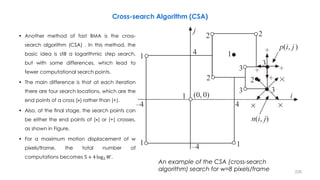

![236
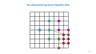
2D-Log Search, Example
3 5 4 5
3 2 5 5 5
4
3
2 1 2
1 1 1
1
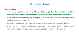
n denotes a search point of step n
i 6 i 5 i 4 i 3 i 2 i 1 i i 1 i 2 i 3 i 4 i 5 i 6 j 6
j 5
j 4
j 3
j 2
j 1
j
j 1
j 2
j 3
j 4
j 5
j 6
The best matching MVs in steps 1– 5 are
(0,2), (0,4), (2,4), (2,6), and (2,6). The final
MV is (2,6). From [Musmann85].](https://image.slidesharecdn.com/videocompressionpart2section2videocodingconceptsbymr-200411173523/85/Video-Compression-Part-2-Section-2-Video-Coding-Concepts-236-320.jpg)


![258
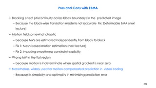
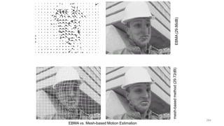
Problems with DBMA
• Motion discontinuity across block boundaries, because nodal MVs are estimated
independently from block to block
– Fix: mesh-based motion estimation
– First apply EBMA to all blocks
• Cannot do well on blocks with multiple moving objects or changes due to illumination
effect
– Three mode method
• First apply EBMA to all blocks
• Blocks with small EBMA errors have translational motion
• Blocks with large EBMA errors may have non-translational motion
– First apply DBMA to these blocks
– Blocks still having errors are non-motion compensable
• [Ref] O. Lee and Y. Wang, Motion compensated prediction using nodal based deformable block matching. J.
Visual Communications and Image Representation (March 1995), 6:26-34](https://image.slidesharecdn.com/videocompressionpart2section2videocodingconceptsbymr-200411173523/85/Video-Compression-Part-2-Section-2-Video-Coding-Concepts-258-320.jpg)
![− Rarely used in practice: BME/BMC mostly suffices
− Reference frame resampling: an option in H.263+/H.263++
− Global affine motion model: special-effect warping
− 3D subband & wavelet coding: align frames before temporal filtering [Taubman]
268
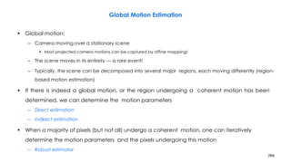
Global Motion Estimation
MV00
MV10 MV11
MV01](https://image.slidesharecdn.com/videocompressionpart2section2videocodingconceptsbymr-200411173523/85/Video-Compression-Part-2-Section-2-Video-Coding-Concepts-268-320.jpg)
![Unrestricted Motion Vector (UMV) (Details in H.263 Codec)
− Improve motion accuracy
− Motion vector range is extended from [-16, 15.5] to [-31.5, 31.5] (as example)
− Motion vector can point outside of the frame
− Closest edge pixel is used (edge pixel is repeated)
− UMV dramatically improves motion estimation when moving objects are entering/exiting the
frame or moving around the frame border)
276
Target Frame NReference Frame N-1
Edge pixels
are repeated.](https://image.slidesharecdn.com/videocompressionpart2section2videocodingconceptsbymr-200411173523/85/Video-Compression-Part-2-Section-2-Video-Coding-Concepts-276-320.jpg)


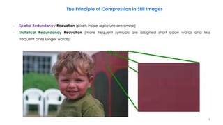
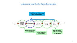
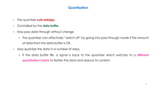
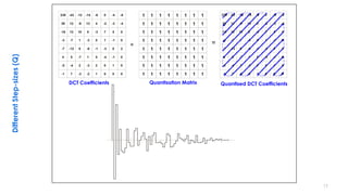
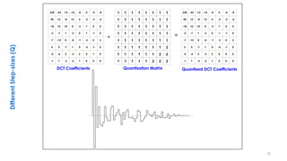
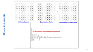
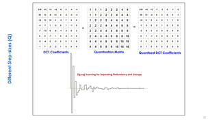
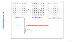
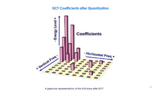
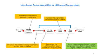
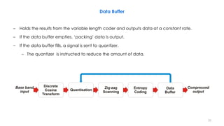
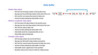
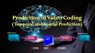
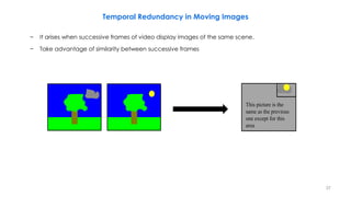
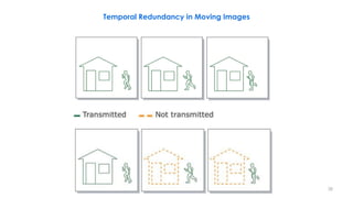
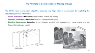
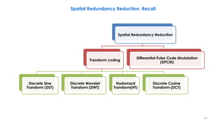
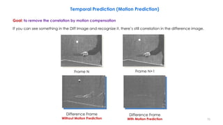
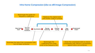
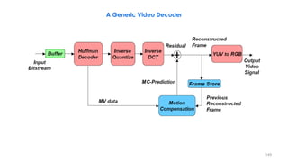
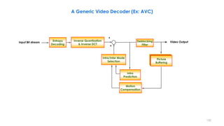
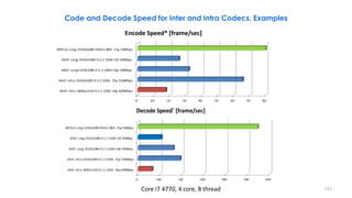
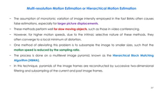
This document discusses video compression techniques. It begins by outlining the history of video compression and describing the basic components of a generic video encoder/decoder system. It then covers specific compression methods including differential pulse code modulation, transform coding using discrete cosine transform, quantization, and entropy coding. The document also discusses techniques for reducing both spatial and temporal redundancy in video, such as prediction coding. It provides examples of how quantization is used to control quality and compression ratio in both lossy and lossless compression systems.