This document provides solutions to problems from Chapter 1 of an electromagnetism textbook. It solves for vectors, vector operations, vector fields and their properties at different points. Some key points solved include finding unit vectors, magnitudes of vectors, angles between vectors, vector projections, and visualizing vector fields. The document contains step-by-step workings for 12 multi-part problems involving concepts of vector algebra and vector calculus.

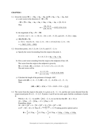
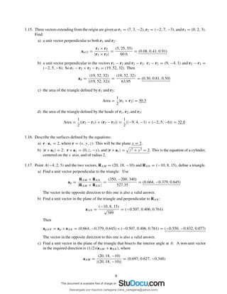
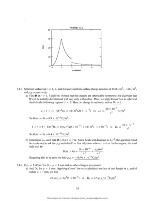
![1.12. Given points A(10, 12, −6), B(16, 8, −2), C(8, 1, −4), and D(−2, −5, 8), determine:
a) the vector projection of RAB + RBC on RAD: RAB + RBC = RAC = (8, 1, 4) − (10, 12, −6) =
(−2, −11, 10) Then RAD = (−2, −5, 8) − (10, 12, −6) = (−12, −17, 14). So the projection will
be:
(RAC · aRAD)aRAD = (−2, −11, 10) ·
(−12, −17, 14)
√
629
(−12, −17, 14)
√
629
= (−6.7, −9.5, 7.8)
b) the vector projection of RAB + RBC on RDC: RDC = (8, −1, 4) − (−2, −5, 8) = (10, 6, −4). The
projection is:
(RAC · aRDC)aRDC = (−2, −11, 10) ·
(10, 6, −4)
√
152
(10, 6, −4)
√
152
= (−8.3, −5.0, 3.3)
c) the angle between RDA and RDC: Use RDA = −RAD = (12, 17, −14) and RDC = (10, 6, −4).
The angle is found through the dot product of the associated unit vectors, or:
θD = cos−1
(aRDA · aRDC) = cos−1 (12, 17, −14) · (10, 6, −4)
√
629
√
152
= 26◦
1.13. a) Find the vector component of F = (10, −6, 5) that is parallel to G = (0.1, 0.2, 0.3):
F||G =
F · G
|G|2
G =
(10, −6, 5) · (0.1, 0.2, 0.3)
0.01 + 0.04 + 0.09
(0.1, 0.2, 0.3) = (0.93, 1.86, 2.79)
b) Find the vector component of F that is perpendicular to G:
FpG = F − F||G = (10, −6, 5) − (0.93, 1.86, 2.79) = (9.07, −7.86, 2.21)
c) Find the vector component of G that is perpendicular to F:
GpF = G−G||F = G−
G · F
|F|2
F = (0.1, 0.2, 0.3)−
1.3
100 + 36 + 25
(10, −6, 5) = (0.02, 0.25, 0.26)
1.14. The four vertices of a regular tetrahedron are located at O(0, 0, 0), A(0, 1, 0), B(0.5
√
3, 0.5, 0), and
C(
√
3/6, 0.5,
√
2/3).
a) Find a unit vector perpendicular (outward) to the face ABC: First find
RBA × RBC = [(0, 1, 0) − (0.5
√
3, 0.5, 0)] × [(
√
3/6, 0.5, 2/3) − (0.5
√
3, 0.5, 0)]
= (−0.5
√
3, 0.5, 0) × (−
√
3/3, 0, 2/3) = (0.41, 0.71, 0.29)
The required unit vector will then be:
RBA × RBC
|RBA × RBC|
= (0.47, 0.82, 0.33)
b) Find the area of the face ABC:
Area =
1
2
|RBA × RBC| = 0.43
5
Descargado por mauricio cartagena (rene_cartagena@yahoo.com)
lOMoARcPSD|5423334](https://image.slidesharecdn.com/solucionario-teoria-electromagnetica-hayt-2001-201211183707/85/Solucionario-teoria-electromagnetica-hayt-2001-7-320.jpg)
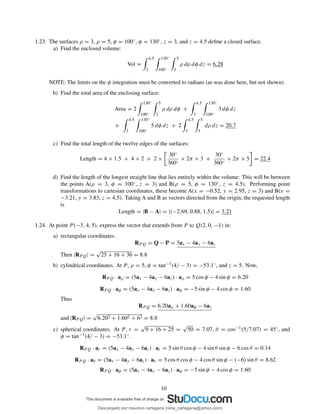
![1.17c. (continued) Now
1
2
(aAM + aAN ) =
1
2
[(0.697, 0.627, −0.348) + (−0.507, 0.406, 0.761)] = (0.095, 0.516, 0.207)
Finally,
abis =
(0.095, 0.516, 0.207)
|(0.095, 0.516, 0.207)|
= (0.168, 0.915, 0.367)
1.18. Given points A(ρ = 5, φ = 70◦, z = −3) and B(ρ = 2, φ = −30◦, z = 1), find:
a) unit vector in cartesian coordinates at A toward B: A(5 cos 70◦, 5 sin 70◦, −3) = A(1.71, 4.70, −3), In
the same manner, B(1.73, −1, 1). So RAB = (1.73, −1, 1) − (1.71, 4.70, −3) = (0.02, −5.70, 4) and
therefore
aAB =
(0.02, −5.70, 4)
|(0.02, −5.70, 4)|
= (0.003, −0.82, 0.57)
b) a vector in cylindrical coordinates at A directed toward B: aAB · aρ = 0.003 cos 70◦ − 0.82 sin 70◦ =
−0.77. aAB · aφ = −0.003 sin 70◦ − 0.82 cos 70◦ = −0.28. Thus
aAB = −0.77aρ − 0.28aφ + 0.57az
.
c) a unit vector in cylindrical coordinates at B directed toward A:
Use aBA = (−0, 003, 0.82, −0.57). Then aBA ·aρ = −0.003 cos(−30◦)+0.82 sin(−30◦) = −0.43, and
aBA · aφ = 0.003 sin(−30◦) + 0.82 cos(−30◦) = 0.71. Finally,
aBA = −0.43aρ + 0.71aφ − 0.57az
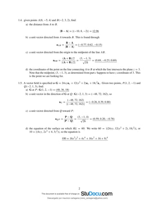
1.19 a) Express the field D = (x2 + y2)−1(xax + yay) in cylindrical components and cylindrical variables:
Have x = ρ cos φ, y = ρ sin φ, and x2 + y2 = ρ2. Therefore
D =
1
ρ
(cos φax + sin φay)
Then
Dρ = D · aρ =
1
ρ
cos φ(ax · aρ) + sin φ(ay · aρ) =
1
ρ
cos2
φ + sin2
φ =
1
ρ
and
Dφ = D · aφ =
1
ρ
cos φ(ax · aφ) + sin φ(ay · aφ) =
1
ρ
[cos φ(− sin φ) + sin φ cos φ] = 0
Therefore
D =
1
ρ
aρ
7
Descargado por mauricio cartagena (rene_cartagena@yahoo.com)
lOMoARcPSD|5423334](https://image.slidesharecdn.com/solucionario-teoria-electromagnetica-hayt-2001-201211183707/85/Solucionario-teoria-electromagnetica-hayt-2001-9-320.jpg)
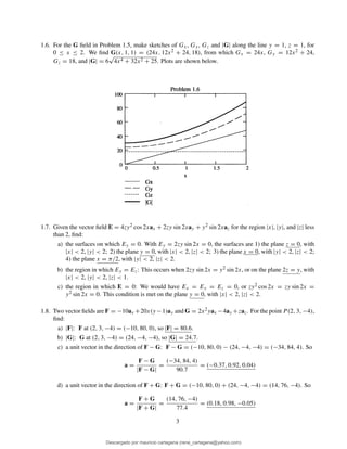
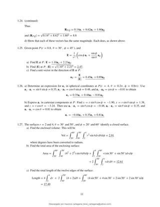
![1.19b. Evaluate D at the point where ρ = 2, φ = 0.2π, and z = 5, expressing the result in cylindrical and
cartesian coordinates: At the given point, and in cylindrical coordinates, D = 0.5aρ. To express this in
cartesian, we use
D = 0.5(aρ · ax)ax + 0.5(aρ · ay)ay = 0.5 cos 36◦
ax + 0.5 sin 36◦
ay = 0.41ax + 0.29ay
1.20. Express in cartesian components:
a) the vector at A(ρ = 4, φ = 40◦, z = −2) that extends to B(ρ = 5, φ = −110◦, z = 2): We
have A(4 cos 40◦, 4 sin 40◦, −2) = A(3.06, 2.57, −2), and B(5 cos(−110◦), 5 sin(−110◦), 2) =
B(−1.71, −4.70, 2) in cartesian. Thus RAB = (−4.77, −7.30, 4).
b) a unit vector at B directed toward A: Have RBA = (4.77, 7.30, −4), and so
aBA =
(4.77, 7.30, −4)
|(4.77, 7.30, −4)|
= (0.50, 0.76, −0.42)
c) a unit vector at B directed toward the origin: Have rB = (−1.71, −4.70, 2), and so −rB =
(1.71, 4.70, −2). Thus
a =
(1.71, 4.70, −2)
|(1.71, 4.70, −2)|
= (0.32, 0.87, −0.37)
1.21. Express in cylindrical components:
a) the vector from C(3, 2, −7) to D(−1, −4, 2):
C(3, 2, −7) → C(ρ = 3.61, φ = 33.7◦, z = −7) and
D(−1, −4, 2) → D(ρ = 4.12, φ = −104.0◦, z = 2).
Now RCD = (−4, −6, 9) and Rρ = RCD · aρ = −4 cos(33.7) − 6 sin(33.7) = −6.66. Then
Rφ = RCD · aφ = 4 sin(33.7) − 6 cos(33.7) = −2.77. So RCD = −6.66aρ − 2.77aφ + 9az
b) a unit vector at D directed toward C:
RCD = (4, 6, −9) and Rρ = RDC · aρ = 4 cos(−104.0) + 6 sin(−104.0) = −6.79. Then Rφ =
RDC · aφ = 4[− sin(−104.0)] + 6 cos(−104.0) = 2.43. So RDC = −6.79aρ + 2.43aφ − 9az
Thus aDC = −0.59aρ + 0.21aφ − 0.78az
c) a unit vector at D directed toward the origin: Start with rD = (−1, −4, 2), and so the vector toward
the origin will be −rD = (1, 4, −2). Thus in cartesian the unit vector is a = (0.22, 0.87, −0.44).
Convert to cylindrical:
aρ = (0.22, 0.87, −0.44) · aρ = 0.22 cos(−104.0) + 0.87 sin(−104.0) = −0.90, and
aφ = (0.22, 0.87, −0.44) · aφ = 0.22[− sin(−104.0)] + 0.87 cos(−104.0) = 0, so that finally,
a = −0.90aρ − 0.44az.
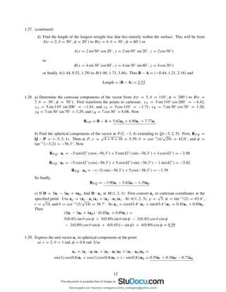
1.22. A field is given in cylindrical coordinates as
F =
40
ρ2 + 1
+ 3(cos φ + sin φ) aρ + 3(cos φ − sin φ)aφ − 2az
where the magnitude of F is found to be:
|F| =
√
F · F =
1600
(ρ2 + 1)2
+
240
ρ2 + 1
(cos φ + sin φ) + 22
1/2
8
Descargado por mauricio cartagena (rene_cartagena@yahoo.com)
lOMoARcPSD|5423334](https://image.slidesharecdn.com/solucionario-teoria-electromagnetica-hayt-2001-201211183707/85/Solucionario-teoria-electromagnetica-hayt-2001-10-320.jpg)
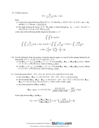
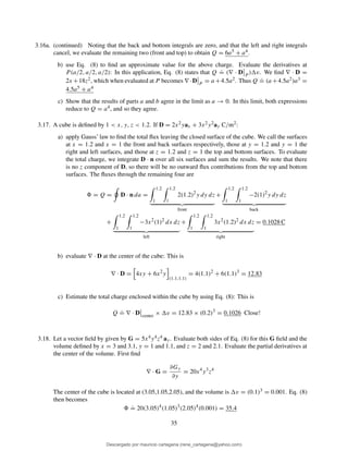
![Sketch |F|:
a) vs. φ with ρ = 3: in this case the above simplifies to
|F(ρ = 3)| = |Fa| = [38 + 24(cos φ + sin φ)]1/2
b) vs. ρ with φ = 0, in which:
|F(φ = 0)| = |Fb| =
1600
(ρ2 + 1)2
+
240
ρ2 + 1
+ 22
1/2
c) vs. ρ with φ = 45◦, in which
|F(φ = 45◦
)| = |Fc| =
1600
(ρ2 + 1)2
+
240
√
2
ρ2 + 1
+ 22
1/2
9
Descargado por mauricio cartagena (rene_cartagena@yahoo.com)
lOMoARcPSD|5423334](https://image.slidesharecdn.com/solucionario-teoria-electromagnetica-hayt-2001-201211183707/85/Solucionario-teoria-electromagnetica-hayt-2001-11-320.jpg)
![CHAPTER 2
2.1. Four 10nC positive charges are located in the z = 0 plane at the corners of a square 8cm on a side.
A fifth 10nC positive charge is located at a point 8cm distant from the other charges. Calculate the
magnitude of the total force on this fifth charge for ǫ = ǫ0:
Arrange the charges in the xy plane at locations (4,4), (4,-4), (-4,4), and (-4,-4). Then the fifth charge
will be on the z axis at location z = 4
√
2, which puts it at 8cm distance from the other four. By
symmetry, the force on the fifth charge will be z-directed, and will be four times the z component of
force produced by each of the four other charges.
F =
4
√
2
×
q2
4πǫ0d2
=
4
√
2
×
(10−8)2
4π(8.85 × 10⁻¹²)(0.08)2
= 4.0 × 10⁻⁴
N
2.2. A charge Q1 = 0.1 µC is located at the origin, while Q2 = 0.2 µC is at A(0.8, −0.6, 0). Find the
locus of points in the z = 0 plane at which the x component of the force on a third positive charge is
zero.
To solve this problem, the z coordinate of the third charge is immaterial, so we can place it in the
xy plane at coordinates (x, y, 0). We take its magnitude to be Q3. The vector directed from the first
charge to the third is R13 = xax + yay; the vector directed from the second charge to the third is
R23 = (x − 0.8)ax + (y + 0.6)ay. The force on the third charge is now
F3 =
Q3
4πǫ0
Q1R13
|R13|3
+
Q2R23
|R23|3
=
Q3 × 10−6
4πǫ0
0.1(xax + yay)
(x2 + y2)1.5
+
0.2[(x − 0.8)ax + (y + 0.6)ay]
[(x − 0.8)2 + (y + 0.6)2]1.5
We desire the x component to be zero. Thus,
0 =
0.1xax
(x2 + y2)1.5
+
0.2(x − 0.8)ax
[(x − 0.8)2 + (y + 0.6)2]1.5
or
x[(x − 0.8)2
+ (y + 0.6)2
]1.5
= 2(0.8 − x)(x2
+ y2
)1.5
2.3. Point charges of 50nC each are located at A(1, 0, 0), B(−1, 0, 0), C(0, 1, 0), and D(0, −1, 0) in free
space. Find the total force on the charge at A.
The force will be:
F =
(50 × 10−9)2
4πǫ0
RCA
|RCA|3
+
RDA
|RDA|3
+
RBA
|RBA|3
where RCA = ax − ay, RDA = ax + ay, and RBA = 2ax. The magnitudes are |RCA| = |RDA| =
√
2,
and |RBA| = 2. Substituting these leads to
F =
(50 × 10−9)2
4πǫ0
1
2
√
2
+
1
2
√
2
+
2
8
ax = 21.5ax µN
where distances are in meters.
14
Descargado por mauricio cartagena (rene_cartagena@yahoo.com)
lOMoARcPSD|5423334](https://image.slidesharecdn.com/solucionario-teoria-electromagnetica-hayt-2001-201211183707/85/Solucionario-teoria-electromagnetica-hayt-2001-16-320.jpg)
![2.4. Let Q1 = 8 µC be located at P1(2, 5, 8) while Q2 = −5 µC is at P2(6, 15, 8). Let ǫ = ǫ0.
a) Find F2, the force on Q2: This force will be
F2 =
Q1Q2
4πǫ0
R12
|R12|3
=
(8 × 10⁻⁶)(−5 × 10⁻⁶)
4πǫ0
(4ax + 10ay)
(116)1.5
= (−1.15ax − 2.88ay) mN
b) Find the coordinates of P3 if a charge Q3 experiences a total force F3 = 0 at P3: This force in
general will be:
F3 =
Q3
4πǫ0
Q1R13
|R13|3
+
Q2R23
|R23|3
where R13 = (x − 2)ax + (y − 5)ay and R23 = (x − 6)ax + (y − 15)ay. Note, however, that
all three charges must lie in a straight line, and the location of Q3 will be along the vector R12
extended past Q2. The slope of this vector is (15 − 5)/(6 − 2) = 2.5. Therefore, we look for P3
at coordinates (x, 2.5x, 8). With this restriction, the force becomes:
F3 =
Q3
4πǫ0
8[(x − 2)ax + 2.5(x − 2)ay]
[(x − 2)2 + (2.5)2(x − 2)2]1.5
−
5[(x − 6)ax + 2.5(x − 6)ay]
[(x − 6)2 + (2.5)2(x − 6)2]1.5
where we require the term in large brackets to be zero. This leads to
8(x − 2)[((2.5)2
+ 1)(x − 6)2
]1.5
− 5(x − 6)[((2.5)2
+ 1)(x − 2)2
]1.5
= 0
which reduces to
8(x − 6)2
− 5(x − 2)2
= 0
or
x =
6
√
8 − 2
√
5
√
8 −
√
5
= 21.1
The coordinates of P3 are thus P3(21.1, 52.8, 8)
2.5. Let a point charge Q125 nC be located at P1(4, −2, 7) and a charge Q2 = 60 nC be at P2(−3, 4, −2).
a) If ǫ = ǫ0, find E at P3(1, 2, 3): This field will be
E =
10−9
4πǫ0
25R13
|R13|3
+
60R23
|R23|3
where R13 = −3ax +4ay −4az and R23 = 4ax −2ay +5az. Also, |R13| =
√
41 and |R23| =
√
45.
So
E =
10−9
4πǫ0
25 × (−3ax + 4ay − 4az)
(41)1.5
+
60 × (4ax − 2ay + 5az)
(45)1.5
= 4.58ax − 0.15ay + 5.51az
b) At what point on the y axis is Ex = 0? P3 is now at (0, y, 0), so R13 = −4ax + (y + 2)ay − 7az
and R23 = 3ax + (y − 4)ay + 2az. Also, |R13| = 65 + (y + 2)2 and |R23| = 13 + (y − 4)2.
Now the x component of E at the new P3 will be:
Ex =
10−9
4πǫ0
25 × (−4)
[65 + (y + 2)2]1.5
+
60 × 3
[13 + (y − 4)2]1.5
To obtain Ex = 0, we require the expression in the large brackets to be zero. This expression
simplifies to the following quadratic:
0.48y2
+ 13.92y + 73.10 = 0
which yields the two values: y = −6.89, −22.11
15
Descargado por mauricio cartagena (rene_cartagena@yahoo.com)
lOMoARcPSD|5423334](https://image.slidesharecdn.com/solucionario-teoria-electromagnetica-hayt-2001-201211183707/85/Solucionario-teoria-electromagnetica-hayt-2001-17-320.jpg)
![2.9. A 100 nC point charge is located at A(−1, 1, 3) in free space.
a) Find the locus of all points P (x, y, z) at which Ex = 500 V/m: The total field at P will be:
EP =
100 × 10−9
4πǫ0
RAP
|RAP |3
where RAP = (x + 1)ax + (y − 1)ay + (z − 3)az, and where |RAP | = [(x + 1)2 + (y − 1)2 +
(z − 3)2]1/2. The x component of the field will be
Ex =
100 × 10−9
4πǫ0
(x + 1)
[(x + 1)2 + (y − 1)2 + (z − 3)2]1.5
= 500 V/m
And so our condition becomes:
(x + 1) = 0.56 [(x + 1)2
+ (y − 1)2
+ (z − 3)2
]1.5
b) Find y1 if P (−2, y1, 3) lies on that locus: At point P , the condition of part a becomes
3.19 = 1 + (y1 − 1)2
3
from which (y1 − 1)2 = 0.47, or y1 = 1.69 or 0.31
2.10. Charges of 20 and -20 nC are located at (3, 0, 0) and (−3, 0, 0), respectively. Let ǫ = ǫ0.
Determine |E| at P (0, y, 0): The field will be
EP =
20 × 10−9
4πǫ0
R1
|R1|3
−
R2
|R2|3
where R1, the vector from the positive charge to point P is (−3, y, 0), and R2, the vector from
the negative charge to point P , is (3, y, 0). The magnitudes of these vectors are |R1| = |R2| =
9 + y2. Substituting these into the expression for EP produces
EP =
20 × 10−9
4πǫ0
−6ax
(9 + y2)1.5
from which
|EP | =
1079
(9 + y2)1.5
V/m
2.11. A charge Q0 located at the origin in free space produces a field for which Ez = 1 kV/m at point
P (−2, 1, −1).
a) Find Q0: The field at P will be
EP =
Q0
4πǫ0
−2ax + ay − az
61.5
Since the z component is of value 1 kV/m, we find Q0 = −4πǫ061.5 × 103 = −1.63 µC.
17
Descargado por mauricio cartagena (rene_cartagena@yahoo.com)
lOMoARcPSD|5423334](https://image.slidesharecdn.com/solucionario-teoria-electromagnetica-hayt-2001-201211183707/85/Solucionario-teoria-electromagnetica-hayt-2001-19-320.jpg)
![2.11. (continued)
b) Find E at M(1, 6, 5) in cartesian coordinates: This field will be:
EM =
−1.63 × 10⁻⁶
4πǫ0
ax + 6ay + 5az
[1 + 36 + 25]1.5
or EM = −30.11ax − 180.63ay − 150.53az.
c) Find E at M(1, 6, 5) in cylindrical coordinates: At M, ρ =
√
1 + 36 = 6.08, φ = tan−1(6/1) =
80.54◦, and z = 5. Now
Eρ = EM · aρ = −30.11 cos φ − 180.63 sin φ = −183.12
Eφ = EM · aφ = −30.11(− sin φ) − 180.63 cos φ = 0 (as expected)
so that EM = −183.12aρ − 150.53az.
d) Find E at M(1, 6, 5) in spherical coordinates: At M, r =
√
1 + 36 + 25 = 7.87, φ = 80.54◦ (as
before), and θ = cos−1(5/7.87) = 50.58◦. Now, since the charge is at the origin, we expect to
obtain only a radial component of EM. This will be:
Er = EM · ar = −30.11 sin θ cos φ − 180.63 sin θ sin φ − 150.53 cos θ = −237.1
2.12. The volume charge density ρv = ρ0e−|x|−|y|−|z| exists over all free space. Calculate the total charge
present: This will be 8 times the integral of ρv over the first octant, or
Q = 8
∞
0
∞
0
∞
0
ρ0e−x−y−z
dx dy dz = 8ρ0
2.13. A uniform volume charge density of 0.2 µC/m3 (note typo in book) is present throughout the spherical
shell extending from r = 3 cm to r = 5 cm. If ρv = 0 elsewhere:
a) find the total charge present throughout the shell: This will be
Q =
2π
0
π
0
.05
.03
0.2 r2
sin θ dr dθ dφ = 4π(0.2)
r3
3
.05
.03
= 8.21 × 10⁻⁵
µC = 82.1 pC
b) find r1 if half the total charge is located in the region 3 cm < r < r1: If the integral over r in part
a is taken to r1, we would obtain
4π(0.2)
r3
3
r1
.03
= 4.105 × 10⁻⁵
Thus
r1 =
3 × 4.105 × 10−5
0.2 × 4π
+ (.03)3
1/3
= 4.24 cm
18
Descargado por mauricio cartagena (rene_cartagena@yahoo.com)
lOMoARcPSD|5423334](https://image.slidesharecdn.com/solucionario-teoria-electromagnetica-hayt-2001-201211183707/85/Solucionario-teoria-electromagnetica-hayt-2001-20-320.jpg)

![2.18. (continued)
b) Find E at Q(2, 3, 4): This field will in general be:
EQ =
ρl
2πǫ0
R+Q
|R+Q|
−
R−Q
|R−Q|
where R+Q = (2, 3, 4)−(0, −.6, 4) = (2, 3.6, 0), and R−Q = (2, 3, 4)−(0, .6, 4) = (2, 2.4, 0).
Thus
EQ =
ρl
2πǫ0
2ax + 3.6ay
22 + (3.6)2
−
2ax + 2.4ay
22 + (2.4)2
= −625.8ax − 241.6ay V/m
2.19. A uniform line charge of 2 µC/m is located on the z axis. Find E in cartesian coordinates at P (1, 2, 3)
if the charge extends from
a) −∞ < z < ∞: With the infinite line, we know that the field will have only a radial component
in cylindrical coordinates (or x and y components in cartesian). The field from an infinite line on
the z axis is generally E = [ρl/(2πǫ0ρ)]aρ. Therefore, at point P :
EP =
ρl
2πǫ0
RzP
|RzP |2
=
(2 × 10⁻⁶)
2πǫ0
ax + 2ay
5
= 7.2ax + 14.4ay kV/m
where RzP is the vector that extends from the line charge to point P, and is perpendicular to the z
axis; i.e., RzP = (1, 2, 3) − (0, 0, 3) = (1, 2, 0).
b) −4 ≤ z ≤ 4: Here we use the general relation
EP =
ρldz
4πǫ0
r − r′
|r − r′|3
where r = ax + 2ay + 3az and r′ = zaz. So the integral becomes
EP =
(2 × 10⁻⁶)
4πǫ0
4
−4
ax + 2ay + (3 − z)az
[5 + (3 − z)2]1.5
dz
Using integral tables, we obtain:
EP = 3597
(ax + 2ay)(z − 3) + 5az
(z2 − 6z + 14)
4
−4
V/m = 4.9ax + 9.8ay + 4.9az kV/m
The student is invited to verify that when evaluating the above expression over the limits −∞ <
z < ∞, the z component vanishes and the x and y components become those found in part a.
2.20. Uniform line charges of 120 nC/m lie along the entire extent of the three coordinate axes. Assuming
free space conditions, find E at P (−3, 2, −1): Since all line charges are infinitely-long, we can write:
EP =
ρl
2πǫ0
RxP
|RxP |2
+
RyP
|RyP |2
+
RzP
|RzP |2
where RxP , RyP , and RzP are the normal vectors from each of the three axes that terminate on point
P . Specifically, RxP = (−3, 2, −1) − (−3, 0, 0) = (0, 2, −1), RyP = (−3, 2, −1) − (0, 2, 0) =
(−3, 0, −1), and RzP = (−3, 2, −1) − (0, 0, −1) = (−3, 2, 0). Substituting these into the expression
for EP gives
EP =
ρl
2πǫ0
2ay − az
5
+
−3ax − az
10
+
−3ax + 2ay
13
= −1.15ax + 1.20ay − 0.65az kV/m
21
Descargado por mauricio cartagena (rene_cartagena@yahoo.com)
lOMoARcPSD|5423334](https://image.slidesharecdn.com/solucionario-teoria-electromagnetica-hayt-2001-201211183707/85/Solucionario-teoria-electromagnetica-hayt-2001-23-320.jpg)
![2.21. Two identical uniform line charges with ρl = 75 nC/m are located in free space at x = 0, y = ±0.4 m.
What force per unit length does each line charge exert on the other? The charges are parallel to the z
axis and are separated by 0.8 m. Thus the field from the charge at y = −0.4 evaluated at the location
of the charge at y = +0.4 will be E = [ρl/(2πǫ0(0.8))]ay. The force on a differential length of the
line at the positive y location is dF = dqE = ρldzE. Thus the force per unit length acting on the line
at postive y arising from the charge at negative y is
F =
1
0
ρ2
l dz
2πǫ0(0.8)
ay = 1.26 × 10⁻⁴
ay N/m = 126 ay µN/m
The force on the line at negative y is of course the same, but with −ay.
2.22. A uniform surface charge density of 5 nC/m2 is present in the region x = 0, −2 < y < 2, and all z. If
ǫ = ǫ0, find E at:
a) PA(3, 0, 0): We use the superposition integral:
E =
ρsda
4πǫ0
r − r′
|r − r′|3
where r = 3ax and r′ = yay + zaz. The integral becomes:
EP A =
ρs
4πǫ0
∞
−∞
2
−2
3ax − yay − zaz
[9 + y2 + z2]1.5
dy dz
Since the integration limits are symmetric about the origin, and since the y and z components of
the integrand exhibit odd parity (change sign when crossing the origin, but otherwise symmetric),
these will integrate to zero, leaving only the x component. This is evident just from the symmetry
of the problem. Performing the z integration first on the x component, we obtain (using tables):
Ex,PA =
3ρs
4πǫ0
2
−2
dy
(9 + y2)
z
9 + y2 + z2
∞
−∞
=
3ρs
2πǫ0
2
−2
dy
(9 + y2)
=
3ρs
2πǫ0
1
3
tan−1 y
3
2
−2 = 106 V/m
The student is encouraged to verify that if the y limits were −∞ to ∞, the result would be that of
the infinite charged plane, or Ex = ρs/(2ǫ0).
b) PB(0, 3, 0): In this case, r = 3ay, and symmetry indicates that only a y component will exist.
The integral becomes
Ey,P B =
ρs
4πǫ0
∞
−∞
2
−2
(3 − y) dy dz
[(z2 + 9) − 6y + y2]1.5
=
ρs
2πǫ0
2
−2
(3 − y) dy
(3 − y)2
= −
ρs
2πǫ0
ln(3 − y) 2
−2 = 145 V/m
22
Descargado por mauricio cartagena (rene_cartagena@yahoo.com)
lOMoARcPSD|5423334](https://image.slidesharecdn.com/solucionario-teoria-electromagnetica-hayt-2001-201211183707/85/Solucionario-teoria-electromagnetica-hayt-2001-24-320.jpg)
![2.27. Given the electric field E = (4x − 2y)ax − (2x + 4y)ay, find:
a) the equation of the streamline that passes through the point P (2, 3, −4): We write
dy
dx
=
Ey
Ex
=
−(2x + 4y)
(4x − 2y)
Thus
2(x dy + y dx) = y dy − x dx
or
2 d(xy) =
1
2
d(y2
) −
1
2
d(x2
)
So
C1 + 2xy =
1
2
y2
−
1
2
x2
or
y2
− x2
= 4xy + C2
Evaluating at P (2, 3, −4), obtain:
9 − 4 = 24 + C2, or C2 = −19
Finally, at P , the requested equation is
y2
− x2
= 4xy − 19
b) a unit vector specifying the direction of E at Q(3, −2, 5): Have EQ = [4(3) + 2(2)]ax − [2(3) −
4(2)]ay = 16ax + 2ay. Then |E| =
√
162 + 4 = 16.12 So
aQ =
16ax + 2ay
16.12
= 0.99ax + 0.12ay
2.28. Let E = 5x3 ax − 15x2y ay, and find:
a) the equation of the streamline that passes through P (4, 2, 1): Write
dy
dx
=
Ey
Ex
=
−15x2y
5x3
=
−3y
x
So
dy
y
= −3
dx
x
⇒ ln y = −3 ln x + ln C
Thus
y = e−3 ln x
eln C
=
C
x3
At P , have 2 = C/(4)3 ⇒ C = 128. Finally, at P ,
y =
128
x3
24
Descargado por mauricio cartagena (rene_cartagena@yahoo.com)
lOMoARcPSD|5423334](https://image.slidesharecdn.com/solucionario-teoria-electromagnetica-hayt-2001-201211183707/85/Solucionario-teoria-electromagnetica-hayt-2001-26-320.jpg)
![3.2c. (continued) The total charge enclosed in the sphere (and the outward flux from it) is now
Ql + Qp = 2(1.94)(−50 × 10−9
) + 2(1.73)(80 × 10−9
) + 12 × 10−9
= 348 nC
3.3. The cylindrical surface ρ = 8 cm contains the surface charge density, ρs = 5e−20|z| nC/m2.
a) What is the total amount of charge present? We integrate over the surface to find:
Q = 2
∞
0
2π
0
5e−20z
(.08)dφ dz nC = 20π(.08)
−1
20
e−20z
∞
0
= 0.25 nC
b) How much flux leaves the surface ρ = 8 cm, 1 cm < z < 5cm, 30◦ < φ < 90◦? We just integrate
the charge density on that surface to find the flux that leaves it.
= Q′
=
.05
.01
90◦
30◦
5e−20z
(.08) dφ dz nC =
90 − 30
360
2π(5)(.08)
−1
20
e−20z
.05
.01
= 9.45 × 10⁻³
nC = 9.45 pC
3.4. The cylindrical surfaces ρ = 1, 2, and 3 cm carry uniform surface charge densities of 20, −8, and 5
nC/m2, respectively.
a) How much electric flux passes through the closed surface ρ = 5 cm, 0 < z < 1 m? Since the
densities are uniform, the flux will be
= 2π(aρs1 + bρs2 + cρs3)(1 m) = 2π [(.01)(20) − (.02)(8) + (.03)(5)] × 10−9
= 1.2 nC
b) Find D at P (1 cm, 2 cm, 3 cm): This point lies at radius
√
5 cm, and is thus inside the outermost
charge layer. This layer, being of uniform density, will not contribute to D at P . We know that in
cylindrical coordinates, the layers at 1 and 2 cm will produce the flux density:
D = Dρaρ =
aρs1 + bρs2
ρ
aρ
or
Dρ =
(.01)(20) + (.02)(−8)
√
.05
= 1.8 nC/m2
At P , φ = tan−1(2/1) = 63.4◦. Thus Dx = 1.8 cos φ = 0.8 and Dy = 1.8 sin φ = 1.6. Finally,
DP = (0.8ax + 1.6ay) nC/m2
28
Descargado por mauricio cartagena (rene_cartagena@yahoo.com)
lOMoARcPSD|5423334](https://image.slidesharecdn.com/solucionario-teoria-electromagnetica-hayt-2001-201211183707/85/Solucionario-teoria-electromagnetica-hayt-2001-30-320.jpg)
![3.5. Let D = 4xyax + 2(x2 + z2)ay + 4yzaz C/m2 and evaluate surface integrals to find the total charge
enclosed in the rectangular parallelepiped 0 < x < 2, 0 < y < 3, 0 < z < 5 m: Of the 6 surfaces to
consider, only 2 will contribute to the net outward flux. Why? First consider the planes at y = 0 and 3.
The y component of D will penetrate those surfaces, but will be inward at y = 0 and outward at y = 3,
while having the same magnitude in both cases. These fluxes will thus cancel. At the x = 0 plane,
Dx = 0 and at the z = 0 plane, Dz = 0, so there will be no flux contributions from these surfaces.
This leaves the 2 remaining surfaces at x = 2 and z = 5. The net outward flux becomes:
=
5
0
3
0
D x=2
· ax dy dz +
3
0
2
0
D z=5
· az dx dy
= 5
3
0
4(2)y dy + 2
3
0
4(5)y dy = 360 C
3.6. Two uniform line charges, each 20 nC/m, are located at y = 1, z = ±1 m. Find the total flux leaving a
sphere of radius 2 m if it is centered at
a) A(3, 1, 0): The result will be the same if we move the sphere to the origin and the line charges to
(0, 0, ±1). The length of the line charge within the sphere is given by l = 4 sin[cos−1(1/2)] =
3.46. With two line charges, symmetrically arranged, the total charge enclosed is given by Q =
2(3.46)(20 nC/m) = 139 nC
b) B(3, 2, 0): In this case the result will be the same if we move the sphere to the origin and keep
the charges where they were. The length of the line joining the origin to the midpoint of the line
charge (in the yz plane) is l1 =
√
2. The length of the line joining the origin to either endpoint
of the line charge is then just the sphere radius, or 2. The half-angle subtended at the origin by
the line charge is then ψ = cos−1(
√
2/2) = 45◦. The length of each line charge in the sphere
is then l2 = 2 × 2 sin ψ = 2
√
2. The total charge enclosed (with two line charges) is now
Q′ = 2(2
√
2)(20 nC/m) = 113 nC
3.7. Volume charge density is located in free space as ρv = 2e−1000r nC/m3 for 0 < r < 1 mm, and ρv = 0
elsewhere.
a) Find the total charge enclosed by the spherical surface r = 1 mm: To find the charge we integrate:
Q =
2π
0
π
0
.001
0
2e−1000r
r2
sin θ dr dθ dφ
Integration over the angles gives a factor of 4π. The radial integration we evaluate using tables;
we obtain
Q = 8π
−r2e−1000r
1000
.001
0
+
2
1000
e−1000r
(1000)2
(−1000r − 1)
.001
0
= 4.0 × 10⁻⁹
nC
b) By using Gauss’s law, calculate the value of Dr on the surface r = 1 mm: The gaussian surface
is a spherical shell of radius 1 mm. The enclosed charge is the result of part a. We thus write
4πr2Dr = Q, or
Dr =
Q
4πr2
=
4.0 × 10⁻⁹
4π(.001)2
= 3.2 × 10⁻⁴
nC/m2
29
Descargado por mauricio cartagena (rene_cartagena@yahoo.com)
lOMoARcPSD|5423334](https://image.slidesharecdn.com/solucionario-teoria-electromagnetica-hayt-2001-201211183707/85/Solucionario-teoria-electromagnetica-hayt-2001-31-320.jpg)
![3.8. Uniform line charges of 5 nC/m ar located in free space at x = 1, z = 1, and at y = 1, z = 0.
a) Obtain an expression for D in cartesian coordinates at P (0, 0, z). In general, we have
D(z) =
ρs
2π
r1 − r′
1
|r1 − r′
1|2
+
r2 − r′
2
|r2 − r′
2|2
where r1 = r2 = zaz, r′
1 = ay, and r′
2 = ax + az. Thus
D(z) =
ρs
2π
[zaz − ay]
[1 + z2]
+
[(z − 1)az − ax]
[1 + (z − 1)2]
=
ρs
2π
−ax
[1 + (z − 1)2]
−
ay
[1 + z2]
+
(z − 1)
[1 + (z − 1)2]
+
z
[1 + z2]
az
b) Plot |D| vs. z at P , −3 < z < 10: Using part a, we find the magnitude of D to be
|D| =
ρs
2π
1
[1 + (z − 1)2]2
+
1
[1 + z2]2
+
(z − 1)
[1 + (z − 1)2]
+
z
[1 + z2]
2 1/2
A plot of this over the specified range is shown in Prob3.8.pdf.
3.9. A uniform volume charge density of 80 µC/m3 is present throughout the region 8 mm < r < 10 mm.
Let ρv = 0 for 0 < r < 8 mm.
a) Find the total charge inside the spherical surface r = 10 mm: This will be
Q =
2π
0
π
0
.010
.008
(80 × 10−6
)r2
sin θ dr dθ dφ = 4π × (80 × 10−6
)
r3
3
.010
.008
= 1.64 × 10⁻¹⁰
C = 164 pC
b) Find Dr at r = 10 mm: Using a spherical gaussian surface at r = 10, Gauss’ law is written as
4πr2Dr = Q = 164 × 10−12, or
Dr(10 mm) =
164 × 10−12
4π(.01)2
= 1.30 × 10⁻⁷
C/m2
= 130 nC/m2
c) If there is no charge for r > 10 mm, find Dr at r = 20 mm: This will be the same computation
as in part b, except the gaussian surface now lies at 20 mm. Thus
Dr(20 mm) =
164 × 10−12
4π(.02)2
= 3.25 × 10⁻⁸
C/m2
= 32.5 nC/m2
3.10. Let ρs = 8 µC/m2 in the region where x = 0 and −4 < z < 4 m, and let ρs = 0 elsewhere. Find D at
P (x, 0, z), where x > 0: The sheet charge can be thought of as an assembly of infinitely-long parallel
strips that lie parallel to the y axis in the yz plane, and where each is of thickness dz. The field from
each strip is that of an infinite line charge, and so we can construct the field at P from a single strip as:
dDP =
ρs dz′
2π
r − r′
|r − r′|2
30
Descargado por mauricio cartagena (rene_cartagena@yahoo.com)
lOMoARcPSD|5423334](https://image.slidesharecdn.com/solucionario-teoria-electromagnetica-hayt-2001-201211183707/85/Solucionario-teoria-electromagnetica-hayt-2001-32-320.jpg)
![3.10 (continued) where r = xax + zaz and r′ = z′az We distinguish between the fixed coordinate of P , z,
and the variable coordinate, z′, that determines the location of each charge strip. To find the net field at
P, we sum the contributions of each strip by integrating over z′:
DP =
4
−4
8 × 10⁻⁶ dz′ (xax + (z − z′)az)
2π[x2 + (z − z′)2]
We can re-arrange this to determine the integral forms:
DP =
8 × 10⁻⁶
2π
(xax + zaz)
4
−4
dz′
(x2 + z2) − 2zz′ + (z′)2
− az
4
−4
z′ dz′
(x2 + z2) − 2zz′ + (z′)2
Using integral tables, we find
DP =
4 × 10⁻⁶
π
(xax + zaz)
1
x
tan−1 2z′ − 2z
2x
−
1
2
ln(x2
+ z2
− 2zz′
+ (z′
)2
) +
2z
2
1
x
tan−1 2z′ − 2z
2x
az
4
−4
which evaluates as
DP =
4 × 10⁻⁶
π
tan−1 z + 4
x
− tan−1 z − 4
x
ax +
1
2
ln
x2 + (z + 4)2
x2 + (z − 4)2
az C/m2
The student is invited to verify that for very small x or for a very large sheet (allowing z′ to approach
infinity), the above expression reduces to the expected form, DP = ρs/2. Note also that the expression
is valid for all x (positive or negative values).
3.11. In cylindrical coordinates, let ρv = 0 for ρ < 1 mm, ρv = 2 sin(2000πρ) nC/m3 for 1 mm < ρ <
1.5 mm, and ρv = 0 for ρ > 1.5 mm. Find D everywhere: Since the charge varies only with radius,
and is in the form of a cylinder, symmetry tells us that the flux density will be radially-directed and will
be constant over a cylindrical surface of a fixed radius. Gauss’ law applied to such a surface of unit
length in z gives:
a) for ρ < 1 mm, Dρ = 0, since no charge is enclosed by a cylindrical surface whose radius lies
within this range.
b) for 1 mm < ρ < 1.5 mm, we have
2πρDρ = 2π
ρ
.001
2 × 10⁻⁹
sin(2000πρ′
)ρ′
dρ′
= 4π × 10−9 1
(2000π)2
sin(2000πρ) −
ρ
2000π
cos(2000πρ)
ρ
.001
or finally,
Dρ =
10−15
2π2ρ
sin(2000πρ) + 2π 1 − 103
ρ cos(2000πρ) C/m2
(1 mm < ρ < 1.5 mm)
31
Descargado por mauricio cartagena (rene_cartagena@yahoo.com)
lOMoARcPSD|5423334](https://image.slidesharecdn.com/solucionario-teoria-electromagnetica-hayt-2001-201211183707/85/Solucionario-teoria-electromagnetica-hayt-2001-33-320.jpg)
![3.14b. find Dρ for ρ > 1 mm: The Gaussian cylinder now lies outside the charge, so
2πρDρ = π(.001)2
(5 × 10⁻⁹
) ⇒ Dρ =
2.5 × 10⁻¹⁵
ρ
C/m2
c) What line charge ρL at ρ = 0 would give the same result for part b? The line charge field will be
Dr =
ρL
2πρ
=
2.5 × 10⁻¹⁵
ρ
(part b)
Thus ρL = 5π × 10−15 C/m. In all answers, ρ is expressed in meters.
3.15. Volume charge density is located as follows: ρv = 0 for ρ < 1 mm and for ρ > 2 mm, ρv = 4ρ µC/m3
for 1 < ρ < 2 mm.
a) Calculate the total charge in the region 0 < ρ < ρ1, 0 < z < L, where 1 < ρ1 < 2 mm: We find
Q =
L
0
2π
0
ρ1
.001
4ρ ρ dρ dφ dz =
8πL
3
[ρ3
1 − 10−9
] µC
where ρ1 is in meters.
b) Use Gauss’ law to determine Dρ at ρ = ρ1: Gauss’ law states that 2πρ1LDρ = Q, where Q is
the result of part a. Thus
Dρ(ρ1) =
4(ρ3
1 − 10−9)
3ρ1
µC/m2
where ρ1 is in meters.
c) Evaluate Dρ at ρ = 0.8 mm, 1.6 mm, and 2.4 mm: At ρ = 0.8 mm, no charge is enclosed by a
cylindrical gaussian surface of that radius, so Dρ(0.8mm) = 0. At ρ = 1.6 mm, we evaluate the
part b result at ρ1 = 1.6 to obtain:
Dρ(1.6mm) =
4[(.0016)3 − (.0010)3]
3(.0016)
= 3.6 × 10⁻⁶
µC/m2
At ρ = 2.4, we evaluate the charge integral of part a from .001 to .002, and Gauss’ law is written
as
2πρLDρ =
8πL
3
[(.002)2
− (.001)2
] µC
from which Dρ(2.4mm) = 3.9 × 10⁻⁶ µC/m2.
3.16. Given the electric flux density, D = 2xy ax + x2 ay + 6z3 az C/m2:
a) use Gauss’ law to evaluate the total charge enclosed in the volume 0 < x, y, z < a: We call the
surfaces at x = a and x = 0 the front and back surfaces respectively, those at y = a and y = 0
the right and left surfaces, and those at z = a and z = 0 the top and bottom surfaces. To evaluate
the total charge, we integrate D · n over all six surfaces and sum the results:
= Q = D · n da =
a
0
a
0
2ay dy dz
front
+
a
0
a
0
−2(0)y dy dz
back
+
a
0
a
0
−x2
dx dz
left
+
a
0
a
0
x2
dx dz
right
+
a
0
a
0
−6(0)3
dx dy
bottom
+
a
0
a
0
6a3
dx dy
top
34
Descargado por mauricio cartagena (rene_cartagena@yahoo.com)
lOMoARcPSD|5423334](https://image.slidesharecdn.com/solucionario-teoria-electromagnetica-hayt-2001-201211183707/85/Solucionario-teoria-electromagnetica-hayt-2001-36-320.jpg)
![3.22. Let D = 8ρ sin φ aρ + 4ρ cos φ aφ C/m2.
a) Find div D: Using the divergence formula for cylindrical coordinates (see problem 3.21), we find
∇ · D = 12 sin φ.
b) Find the volume charge density at P (2.6, 38◦, −6.1): Since ρv = ∇ · D, we evaluate the result of
part a at this point to find ρvP = 12 sin 38◦ = 7.39 C/m3.
c) How much charge is located inside the region defined by 0 < ρ < 1.8, 20◦ < φ < 70◦,
2.4 < z < 3.1? We use
Q =
vol
ρvdv =
3.1
2.4
70◦
20◦
1.8
0
12 sin φρ dρ dφ dz = −(3.1 − 2.4)12 cos φ
70◦
20◦
ρ2
2
1.8
0
= 8.13 C
3.23. a) A point charge Q lies at the origin. Show that div D is zero everywhere except at the origin. For
a point charge at the origin we know that D = Q/(4πr2) ar. Using the formula for divergence in
spherical coordinates (see problem 3.21 solution), we find in this case that
∇ · D =
1
r2
d
dr
r2 Q
4πr2
= 0
The above is true provided r > 0. When r = 0, we have a singularity in D, so its divergence is not
defined.
b) Replace the point charge with a uniform volume charge density ρv0 for 0 < r < a. Relate ρv0
to Q and a so that the total charge is the same. Find div D everywhere: To achieve the same net
charge, we require that (4/3)πa3ρv0 = Q, so ρv0 = 3Q/(4πa3) C/m3. Gauss’ law tells us that
inside the charged sphere
4πr2
Dr =
4
3
πr3
ρv0 =
Qr3
a3
Thus
Dr =
Qr
4πa3
C/m2
and ∇ · D =
1
r2
d
dr
Qr3
4πa3
=
3Q
4πa3
as expected. Outside the charged sphere, D = Q/(4πr2) ar as before, and the divergence is zero.
3.24. Inside the cylindrical shell, 3 < ρ < 4 m, the electric flux density is given as
D = 5(ρ − 3)3
aρ C/m2
a) What is the volume charge density at ρ = 4 m? In this case we have
ρv = ∇ · D =
1
ρ
d
dρ
(ρDρ) =
1
ρ
d
dρ
[5ρ(ρ − 3)3
] =
5(ρ − 3)2
ρ
(4ρ − 3) C/m3
Evaluating this at ρ = 4 m, we find ρv(4) = 16.25 C/m3
b) What is the electric flux density at ρ = 4 m? We evaluate the given D at this point to find
D(4) = 5 aρ C/m2
37
Descargado por mauricio cartagena (rene_cartagena@yahoo.com)
lOMoARcPSD|5423334](https://image.slidesharecdn.com/solucionario-teoria-electromagnetica-hayt-2001-201211183707/85/Solucionario-teoria-electromagnetica-hayt-2001-39-320.jpg)
![3.24c. How much electric flux leaves the closed surface 3 < ρ < 4, 0 < φ < 2π, −2.5 < z < 2.5? We note
that D has only a radial component, and so flux would leave only through the cylinder sides. Also, D
does not vary with φ or z, so the flux is found by a simple product of the side area and the flux density.
We further note that D = 0 at ρ = 3, so only the outer side (at ρ = 4) will contribute. We use the result
of part b, and write the flux as
= [2.5 − (−2.5)]2π(4)(5) = 200π C
d) How much charge is contained within the volume used in part c? By Gauss’ law, this will be the
same as the net outward flux through that volume, or again, 200π C.
3.25. Within the spherical shell, 3 < r < 4 m, the electric flux density is given as
D = 5(r − 3)3
ar C/m2
a) What is the volume charge density at r = 4? In this case we have
ρv = ∇ · D =
1
r2
d
dr
(r2
Dr) =
5
r
(r − 3)2
(5r − 6) C/m3
which we evaluate at r = 4 to find ρv(r = 4) = 17.50 C/m3.
b) What is the electric flux density at r = 4? Substitute r = 4 into the given expression to
find D(4) = 5 ar C/m2
c) How much electric flux leaves the sphere r = 4? Using the result of part b, this will be =
4π(4)2(5) = 320π C
d) How much charge is contained within the sphere, r = 4? From Gauss’ law, this will be the same
as the outward flux, or again, Q = 320π C.
3.26. Given the field
D =
5 sin θ cos φ
r
ar C/m2
,
find:
a) the volume charge density: Use
ρv = ∇ · D =
1
r2
d
dr
(r2
Dr) =
5 sin θ cos φ
r2
C/m3
b) the total charge contained within the region r < 2 m: To find this, we integrate over the volume:
Q =
2π
0
π
0
2
0
5 sin θ cos φ
r2
r2
sin θ dr dθ dφ
Before plunging into this one notice that the φ integration is of cos φ from zero to 2π. This yields
a zero result, and so the total enclosed charge is Q = 0.
c) the value of D at the surface r = 2: Substituting r = 2 into the given field produces
D(r = 2) =
5
2
sin θ cos φ ar C/m2
38
Descargado por mauricio cartagena (rene_cartagena@yahoo.com)
lOMoARcPSD|5423334](https://image.slidesharecdn.com/solucionario-teoria-electromagnetica-hayt-2001-201211183707/85/Solucionario-teoria-electromagnetica-hayt-2001-40-320.jpg)
![3.29b. Evaluate the surface integral side for the corresponding closed surface: We call the surfaces at x = 3
and x = 2 the front and back surfaces respectively, those at y = 3 and y = 2 the right and left surfaces,
and those at z = 3 and z = 2 the top and bottom surfaces. To evaluate the surface integral side, we
integrate D · n over all six surfaces and sum the results. Note that since the x component of D does not
vary with x, the outward fluxes from the front and back surfaces will cancel each other. The same is
true for the left and right surfaces, since Dy does not vary with y. This leaves only the top and bottom
surfaces, where the fluxes are:
D · dS =
3
2
3
2
−4xy
32
dxdy
top
−
3
2
3
2
−4xy
22
dxdy
bottom
= (9 − 4)(9 − 4)
1
4
−
1
9
= 3.47 C
3.30. If D = 15ρ2 sin 2φ aρ + 10ρ2 cos 2φ aφ C/m2, evaluate both sides of the divergence theorem for the
region 1 < ρ < 2 m, 1 < φ < 2 rad, 1 < z < 2 m: Taking the surface integral side first, the six sides
over which the flux must be evaluated are only four, since there is no z component of D. We are left
with the sides at φ = 1 and φ = 2 rad (left and right sides, respectively), and those at ρ = 1 and ρ = 2
(back and front sides). We evaluate
D · dS =
2
1
2
1
15(2)2
sin(2φ) (2)dφdz
front
−
2
1
2
1
15(1)2
sin(2φ) (1)dφdz
back
−
2
1
2
1
10ρ2
cos(2) dρdz
left
+
2
1
2
1
10ρ2
cos(4) dρdz
right
= 6.93 C
For the volume integral side, we first evaluate the divergence of D, which is
∇ · D =
1
ρ
∂
∂ρ
(15ρ3
sin 2φ) +
1
ρ
∂
∂φ
(10ρ2
cos 2φ) = 25ρ sin 2φ
Next
vol
∇ · D dv =
2
1
2
1
2
1
25ρ sin(2φ) ρdρ dφ dz =
25
3
ρ3
2
1
− cos(2φ)
2
2
1
= 6.93 C
3.31. Given the flux density
D =
16
r
cos(2θ) aθ C/m2
,
use two different methods to find the total charge within the region 1 < r < 2 m, 1 < θ < 2 rad,
1 < φ < 2 rad: We use the divergence theorem and first evaluate the surface integral side. We are
evaluating the net outward flux through a curvilinear “cube”, whose boundaries are defined by the
specified ranges. The flux contributions will be only through the surfaces of constant θ, however, since
D has only a θ component. On a constant-theta surface, the differential area is da = r sin θdrdφ,
where θ is fixed at the surface location. Our flux integral becomes
D · dS = −
2
1
2
1
16
r
cos(2) r sin(1) drdφ
θ=1
+
2
1
2
1
16
r
cos(4) r sin(2) drdφ
θ=2
= −16 [cos(2) sin(1) − cos(4) sin(2)] = −3.91 C
40
Descargado por mauricio cartagena (rene_cartagena@yahoo.com)
lOMoARcPSD|5423334](https://image.slidesharecdn.com/solucionario-teoria-electromagnetica-hayt-2001-201211183707/85/Solucionario-teoria-electromagnetica-hayt-2001-42-320.jpg)
![3.31. (continued) We next evaluate the volume integral side of the divergence theorem, where in this case,
∇ · D =
1
r sin θ
d
dθ
(sin θ Dθ ) =
1
r sin θ
d
dθ
16
r
cos 2θ sin θ =
16
r2
cos 2θ cos θ
sin θ
− 2 sin 2θ
We now evaluate:
vol
∇ · D dv =
2
1
2
1
2
1
16
r2
cos 2θ cos θ
sin θ
− 2 sin 2θ r2
sin θ drdθdφ
The integral simplifies to
2
1
2
1
2
1
16[cos 2θ cos θ − 2 sin 2θ sin θ] drdθdφ = 8
2
1
[3 cos 3θ − cos θ] dθ = −3.91 C
3.32. If D = 2r ar C/m2, find the total electric flux leaving the surface of the cube, 0 < x, y, z < 0.4: This
is where the divergence theorem really saves you time! First find
∇ · D =
1
r2
d
dr
(r2
× 2r) = 6
Then the net outward flux will be
vol
∇ · D dv = 6(0.4)3
= 0.38 C
41
Descargado por mauricio cartagena (rene_cartagena@yahoo.com)
lOMoARcPSD|5423334](https://image.slidesharecdn.com/solucionario-teoria-electromagnetica-hayt-2001-201211183707/85/Solucionario-teoria-electromagnetica-hayt-2001-43-320.jpg)
![CHAPTER 4
4.1. The value of E at P (ρ = 2, φ = 40◦, z = 3) is given as E = 100aρ −200aφ +300az V/m. Determine
the incremental work required to move a 20 µC charge a distance of 6 µm:
a) in the direction of aρ: The incremental work is given by dW = −q E · dL, where in this case,
dL = dρ aρ = 6 × 10⁻⁶ aρ. Thus
dW = −(20 × 10−6
C)(100 V/m)(6 × 10−6
m) = −12 × 10−9
J = −12 nJ
b) in the direction of aφ: In this case dL = 2 dφ aφ = 6 × 10⁻⁶ aφ, and so
dW = −(20 × 10−6
)(−200)(6 × 10⁻⁶
) = 2.4 × 10⁻⁸
J = 24 nJ
c) in the direction of az: Here, dL = dz az = 6 × 10⁻⁶ az, and so
dW = −(20 × 10−6
)(300)(6 × 10⁻⁶
) = −3.6 × 10⁻⁸
J = −36 nJ
d) in the direction of E: Here, dL = 6 × 10⁻⁶ aE, where
aE =
100aρ − 200aφ + 300az
[1002 + 2002 + 3002]1/2
= 0.267 aρ − 0.535 aφ + 0.802 az
Thus
dW = −(20 × 10−6
)[100aρ − 200aφ + 300az] · [0.267 aρ − 0.535 aφ + 0.802 az](6 × 10⁻⁶
)
= −44.9 nJ
e) In the direction of G = 2 ax − 3 ay + 4 az: In this case, dL = 6 × 10⁻⁶ aG, where
aG =
2ax − 3ay + 4az
[22 + 32 + 42]1/2
= 0.371 ax − 0.557 ay + 0.743 az
So now
dW = −(20 × 10−6
)[100aρ − 200aφ + 300az] · [0.371 ax − 0.557 ay + 0.743 az](6 × 10⁻⁶
)
= −(20 × 10−6
) 37.1(aρ · ax) − 55.7(aρ · ay) − 74.2(aφ · ax) + 111.4(aφ · ay)
+ 222.9] (6 × 10⁻⁶
)
where, at P , (aρ · ax) = (aφ · ay) = cos(40◦) = 0.766, (aρ · ay) = sin(40◦) = 0.643, and
(aφ · ax) = − sin(40◦) = −0.643. Substituting these results in
dW = −(20 × 10−6
)[28.4 − 35.8 + 47.7 + 85.3 + 222.9](6 × 10⁻⁶
) = −41.8 nJ
42
Descargado por mauricio cartagena (rene_cartagena@yahoo.com)
lOMoARcPSD|5423334](https://image.slidesharecdn.com/solucionario-teoria-electromagnetica-hayt-2001-201211183707/85/Solucionario-teoria-electromagnetica-hayt-2001-44-320.jpg)
![4.2. Let E = 400ax − 300ay + 500az in the neighborhood of point P (6, 2, −3). Find the incremental work
done in moving a 4-C charge a distance of 1 mm in the direction specified by:
a) ax + ay + az: We write
dW = −qE · dL = −4(400ax − 300ay + 500az) ·
(ax + ay + az)
√
3
(10−3
)
= −
(4 × 10⁻³)
√
3
(400 − 300 + 500) = −1.39 J
b) −2ax + 3ay − az: The computation is similar to that of part a, but we change the direction:
dW = −qE · dL = −4(400ax − 300ay + 500az) ·
(−2ax + 3ay − az)
√
14
(10−3
)
= −
(4 × 10⁻³)
√
14
(−800 − 900 − 500) = 2.35 J
4.3. If E = 120 aρ V/m, find the incremental amount of work done in moving a 50 µm charge a distance
of 2 mm from:
a) P (1, 2, 3) toward Q(2, 1, 4): The vector along this direction will be Q − P = (1, −1, 1) from
which aPQ = [ax − ay + az]/
√
3. We now write
dW = −qE · dL = −(50 × 10−6
) 120aρ ·
(ax − ay + az
√
3
(2 × 10⁻³
)
= −(50 × 10−6
)(120) (aρ · ax) − (aρ · ay)
1
√
3
(2 × 10⁻³
)
At P, φ = tan−1(2/1) = 63.4◦. Thus (aρ · ax) = cos(63.4) = 0.447 and (aρ · ay) = sin(63.4) =
0.894. Substituting these, we obtain dW = 3.1 µJ.
b) Q(2, 1, 4) toward P (1, 2, 3): A little thought is in order here: Note that the field has only a radial
component and does not depend on φ or z. Note also that P and Q are at the same radius (
√
5)
from the z axis, but have different φ and z coordinates. We could just as well position the two
points at the same z location and the problem would not change. If this were so, then moving
along a straight line between P and Q would thus involve moving along a chord of a circle whose
radius is
√
5. Halfway along this line is a point of symmetry in the field (make a sketch to see
this). This means that when starting from either point, the initial force will be the same. Thus the
answer is dW = 3.1 µJ as in part a. This is also found by going through the same procedure as
in part a, but with the direction (roles of P and Q) reversed.
4.4. Find the amount of energy required to move a 6-C charge from the origin to P (3, 1, −1) in the field
E = 2xax − 3y2ay + 4az V/m along the straight-line path x = −3z, y = x + 2z: We set up the
computation as follows, and find the the result does not depend on the path.
W = −q E · dL = −6 (2xax − 3y2
ay + 4az) · (dxax + dyay + dzaz)
= −6
3
0
2xdx + 6
1
0
3y2
dy − 6
−1
0
4dz = −24 J
43
Descargado por mauricio cartagena (rene_cartagena@yahoo.com)
lOMoARcPSD|5423334](https://image.slidesharecdn.com/solucionario-teoria-electromagnetica-hayt-2001-201211183707/85/Solucionario-teoria-electromagnetica-hayt-2001-45-320.jpg)
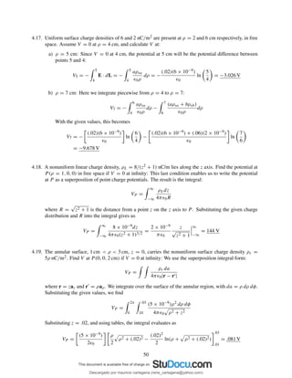
![4.16. Uniform surface charge densities of 6, 4, and 2 nC/m2 are present at r = 2, 4, and 6 cm, respectively,
in free space.
a) Assume V = 0 at infinity, and find V (r). We keep in mind the definition of absolute potential
as the work done in moving a unit positive charge from infinity to location r. At radii outside all
three spheres, the potential will be the same as that of a point charge at the origin, whose charge
is the sum of the three sphere charges:
V (r) (r > 6 cm) =
q1 + q2 + q3
4πǫ0r
=
[4π(.02)2(6) + 4π(.04)2(4) + 4π(.06)2(2)] × 10−9
4πǫ0r
=
(96 + 256 + 288)π × 10−13
4π(8.85 × 10⁻¹²)r
=
1.81
r
V where r is in meters
As the unit charge is moved inside the outer sphere to positions 4 < r < 6 cm, the outer sphere
contribution to the energy is fixed at its value at r = 6. Therefore,
V (r) (4 < r < 6 cm) =
q1 + q2
4πǫ0r
+
q3
4πǫ0(.06)
=
0.994
r
+ 13.6 V
In moving inside the sphere at r = 4 cm, the contribution from that sphere becomes fixed at its
potential function at r = 4:
V (r) (2 < r < 4 cm) =
q1
4πǫ0r
+
q2
4πǫ0(.04)
+
q3
4πǫ0(.06)
=
0.271
r
+ 31.7 V
Finally, using the same reasoning, the potential inside the inner sphere becomes
V (r) (r < 2 cm) =
0.271
.02
+ 31.7 = 45.3 V
b) Calculate V at r = 1, 3, 5, and 7 cm: Using the results of part a, we substitute these distances (in
meters) into the appropriate formulas to obtain: V (1) = 45.3 V,
V (3) = 40.7 V, V (5) = 33.5 V, and V (7) = 25.9 V.
c) Sketch V versus r for 0 < r < 10 cm.
49
Descargado por mauricio cartagena (rene_cartagena@yahoo.com)
lOMoARcPSD|5423334](https://image.slidesharecdn.com/solucionario-teoria-electromagnetica-hayt-2001-201211183707/85/Solucionario-teoria-electromagnetica-hayt-2001-51-320.jpg)
![4.21d. |E|P : taking the magnitude of the part c result, we find |E|P = 75.0 V/m.
e) aN : By definition, this will be
aN
P
= −
E
|E|
= −0.095 ax − 0.304 ay + 0.948 az
f) D: This is D
P
= ǫ0E
P
= 62.8 ax + 202 ay − 629 az pC/m2.
4.22. It is known that the potential is given as V = 80r0.6 V. Assuming free space conditions, find:
a) E: We use
E = −∇V = −
dV
dr
ar = −(0.6)80r−0.4
ar = −48r−0.4
ar V/m
b) the volume charge density at r = 0.5 m: Begin by finding
D = ǫ0E = −48r−0.4
ǫ0 ar C/m2
We next find
ρv = ∇ · D =
1
r2
d
dr
r2
Dr =
1
r2
d
dr
−48ǫ0r1.6
= −
76.8ǫ0
r1.4
C/m3
Then at r = 0.5 m,
ρv(0.5) =
−76.8(8.854 × 10⁻¹²)
(0.5)1.4
= −1.79 × 10⁻⁹
C/m3
= −1.79 nC/m3
c) the total charge lying within the surface r = 0.6: The easiest way is to use Gauss’law, and integrate
the flux density over the spherical surface r = 0.6. Since the field is constant at constant radius,
we obtain the product:
Q = 4π(0.6)2
(−48ǫ0(0.6)−0.4
) = −2.36 × 10⁻⁹
C = −2.36 nC
4.23. It is known that the potential is given as V = 80ρ.6 V. Assuming free space conditions, find:
a) E: We find this through
E = −∇V = −
dV
dρ
aρ = −48ρ−.4
V/m
b) the volume charge density at ρ = .5 m: Using D = ǫ0E, we find the charge density through
ρv
.5
= [∇ · D].5 =
1
ρ
d
dρ
ρDρ
.5
= −28.8ǫ0ρ−1.4
.5
= −673 pC/m3
52
Descargado por mauricio cartagena (rene_cartagena@yahoo.com)
lOMoARcPSD|5423334](https://image.slidesharecdn.com/solucionario-teoria-electromagnetica-hayt-2001-201211183707/85/Solucionario-teoria-electromagnetica-hayt-2001-54-320.jpg)
![4.23c. the total charge lying within the closed surface ρ = .6, 0 < z < 1: The easiest way to do this calculation
is to evaluate Dρ at ρ = .6 (noting that it is constant), and then multiply by the cylinder area: Using part
a, we have Dρ
.6
= −48ǫ0(.6)−.4 = −521 pC/m2. Thus Q = −2π(.6)(1)521×10−12 C = −1.96 nC.
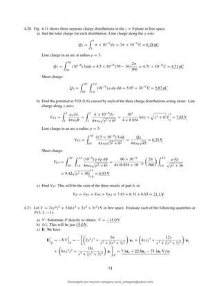
4.24. Given the potential field V = 80r2 cos θ and a point P (2.5, θ = 30◦, φ = 60◦) in free space, find at P :
a) V : Substitute the coordinates into the function and find VP = 80(2.5)2 cos(30) = 433 V.
b) E:
E = −∇V = −
∂V
∂r
ar −
1
r
∂V
∂θ
aθ = −160r cos θar + 80r sin θaθ V/m
Evaluating this at P yields Ep = −346ar + 100aθ V/m.
c) D: In free space, DP = ǫ0EP = (−346ar + 100aθ )ǫ0 = −3.07 ar + 0.885 aθ nC/m2.
d) ρv:
ρv = ∇ · D = ǫ0∇ · E = ǫ0
1
r2
∂
∂r
r2
Er +
1
r2 sin θ
∂
∂θ
(Eθ sin θ)
Substituting the components of E, we find
ρv = −
160 cos θ
r2
3r2
+
1
r sin θ
80r(2 sin θ cos θ) ǫ0 = −320ǫ0 cos θ = −2.45 nC/m3
with θ = 30◦.
e) dV/dN: This will be just |E| evaluated at P , which is
dV
dN P
= | − 346ar + 100aθ | = (346)2 + (100)2 = 360 V/m
f) aN : This will be
aN = −
EP
|EP |
= −
−346ar + 100aθ
(346)2 + (100)2
= 0.961 ar − 0.278 aθ
4.25. Within the cylinder ρ = 2, 0 < z < 1, the potential is given by V = 100 + 50ρ + 150ρ sin φ V.
a) Find V , E, D, and ρv at P (1, 60◦, 0.5) in free space: First, substituting the given point, we find
VP = 279.9 V. Then,
E = −∇V = −
∂V
∂ρ
aρ −
1
ρ
∂V
∂φ
aφ = − [50 + 150 sin φ] aρ − [150 cos φ] aφ
Evaluate the above at P to find EP = −179.9aρ − 75.0aφ V/m
Now D = ǫ0E, so DP = −1.59aρ − .664aφ nC/m2. Then
ρv = ∇ ·D =
1
ρ
d
dρ
ρDρ +
1
ρ
∂Dφ
∂φ
= −
1
ρ
(50 + 150 sin φ) +
1
ρ
150 sin φ ǫ0 = −
50
ρ
ǫ0 C
At P , this is ρvP = −443 pC/m3.
53
Descargado por mauricio cartagena (rene_cartagena@yahoo.com)
lOMoARcPSD|5423334](https://image.slidesharecdn.com/solucionario-teoria-electromagnetica-hayt-2001-201211183707/85/Solucionario-teoria-electromagnetica-hayt-2001-55-320.jpg)
![4.29. A dipole having a moment p = 3ax − 5ay + 10az nC · m is located at Q(1, 2, −4) in free space. Find
V at P (2, 3, 4): We use the general expression for the potential in the far field:
V =
p · (r − r′)
4πǫ0|r − r′|3
where r − r′ = P − Q = (1, 1, 8). So
VP =
(3ax − 5ay + 10az) · (ax + ay + 8az) × 10−9
4πǫ0[12 + 12 + 82]1.5
= 1.31 V
4.30. A dipole, having a moment p = 2az nC · m is located at the origin in free space. Give the magnitude
of E and its direction aE in cartesian components at r = 100 m, φ = 90◦, and θ =: a) 0◦; b) 30◦; c)
90◦. Begin with
E =
p
4πǫ0r3
[2 cos θ ar + sin θ aθ ]
from which
|E| =
p
4πǫ0r3
4 cos2
θ + sin2
θ
1/2
=
p
4πǫ0r3
1 + 3 cos2
θ
1/2
Now
Ex = E · ax =
p
4πǫ0r3
[2 cos θ ar · ax + sin θ aθ · ax] =
p
4πǫ0r3
[3 cos θ sin θ cos φ]
then
Ey = E · ay =
p
4πǫ0r3
2 cos θ ar · ay + sin θ aθ · ay =
p
4πǫ0r3
[3 cos θ sin θ sin φ]
and
Ez = E · az =
p
4πǫ0r3
2 cos θ ar · az + sin θ aθ · az =
p
4πǫ0r3
2 cos2
θ − sin2
θ
Since φ is given as 90◦, Ex = 0, and the field magnitude becomes
|E(φ = 90◦
)| = E2
y + E2
z =
p
4πǫ0r3
9 cos2
θ sin2
θ + (2 cos2
θ − sin2
θ)2
1/2
Then the unit vector becomes (again at φ = 90◦):
aE =
3 cos θ sin θ ay + (2 cos2 θ − sin2 θ) az
9 cos2 θ sin2 θ + (2 cos2 θ − sin2 θ)2 1/2
Now with r = 100 m and p = 2 × 10⁻⁹,
p
4πǫ0r3
=
2 × 10⁻⁹
4π(8.854 × 10⁻¹²)106
= 1.80 × 10⁻⁵
Using the above formulas, we find at θ = 0◦, |E| = (1.80 × 10⁻⁵)(2) = 36.0 µV/m and aE = az.
At θ = 30◦, we find |E| = (1.80 × 10⁻⁵)[1.69 + 1.56]1/2 = 32.5 µV/m and aE = (1.30ay +
1.25az)/1.80 = 0.72 ax + 0.69 az. At θ = 90◦, |E| = (1.80×10⁻⁵)(1) = 18.0 µV/m and aE = −az.
56
Descargado por mauricio cartagena (rene_cartagena@yahoo.com)
lOMoARcPSD|5423334](https://image.slidesharecdn.com/solucionario-teoria-electromagnetica-hayt-2001-201211183707/85/Solucionario-teoria-electromagnetica-hayt-2001-58-320.jpg)
![CHAPTER 5
5.1. Given the current density J = −104[sin(2x)e−2yax + cos(2x)e−2yay] kA/m2:
a) Find the total current crossing the plane y = 1 in the ay direction in the region 0 < x < 1,
0 < z < 2: This is found through
I =
S
J · n
S
da =
2
0
1
0
J · ay
y=1
dx dz =
2
0
1
0
−104
cos(2x)e−2
dx dz
= −104
(2)
1
2
sin(2x)
1
0
e−2
= −1.23 MA
b) Find the total current leaving the region 0 < x, x < 1, 2 < z < 3 by integrating J · dS over
the surface of the cube: Note first that current through the top and bottom surfaces will not exist,
since J has no z component. Also note that there will be no current through the x = 0 plane, since
Jx = 0 there. Current will pass through the three remaining surfaces, and will be found through
I =
3
2
1
0
J · (−ay)
y=0
dx dz +
3
2
1
0
J · (ay)
y=1
dx dz +
3
2
1
0
J · (ax)
x=1
dy dz
= 104
3
2
1
0
cos(2x)e−0
− cos(2x)e−2
dx dz − 104
3
2
1
0
sin(2)e−2y
dy dz
= 104 1
2
sin(2x)
1
0
(3 − 2) 1 − e−2
+ 104 1
2
sin(2)e−2y
1
0
(3 − 2) = 0
c) Repeat part b, but use the divergence theorem: We find the net outward current through the surface
of the cube by integrating the divergence of J over the cube volume. We have
∇ · J =
∂Jx
∂x
+
∂Jy
∂y
= −10−4
2 cos(2x)e−2y
− 2 cos(2x)e−2y
= 0 as expected
5.2. Let the current density be J = 2φ cos2 φaρ − ρ sin 2φaφ A/m2 within the region 2.1 < ρ < 2.5,
0 < φ < 0.1 rad, 6 < z < 6.1. Find the total current I crossing the surface:
a) ρ = 2.2, 0 < φ < 0.1, 6 < z < 6.1 in the aρ direction: This is a surface of constant ρ, so only
the radial component of J will contribute: At ρ = 2.2 we write:
I = J · dS =
6.1
6
0.1
0
2(2) cos2
φ aρ · aρ 2dφdz = 2(2.2)2
(0.1)
0.1
0
1
2
(1 + cos 2φ) dφ
= 0.2(2.2)2 1
2
(0.1) +
1
4
sin 2φ
0.1
0
= 97 mA
b) φ = 0.05, 2.2 < ρ < 2.5, 6 < z < 6.1 in the aφ direction: In this case only the φ component of
J will contribute:
I = J · dS =
6.1
6
2.5
2.2
−ρ sin 2φ φ=0.05
aφ · aφ dρ dz = −(0.1)2 ρ2
2
2.5
2.2
= −7 mA
60
Descargado por mauricio cartagena (rene_cartagena@yahoo.com)
lOMoARcPSD|5423334](https://image.slidesharecdn.com/solucionario-teoria-electromagnetica-hayt-2001-201211183707/85/Solucionario-teoria-electromagnetica-hayt-2001-62-320.jpg)
![5.2c. Evaluate ∇ · J at P (ρ = 2.4, φ = 0.08, z = 6.05):
∇ · J =
1
ρ
∂
∂ρ
(ρJρ) +
1
ρ
∂Jφ
∂φ
=
1
ρ
∂
∂ρ
(2ρ2
cos2
φ) −
1
ρ
∂
∂φ
(ρ sin 2φ) = 4 cos2
φ − 2 cos 2φ
0.08
= 2.0 A/m3
5.3. Let
J =
400 sin θ
r2 + 4
ar A/m2
a) Find the total current flowing through that portion of the spherical surface r = 0.8, bounded by
0.1π < θ < 0.3π, 0 < φ < 2π: This will be
I = J · n
S
da =
2π
0
.3π
.1π
400 sin θ
(.8)2 + 4
(.8)2
sin θ dθ dφ =
400(.8)22π
4.64
.3π
.1π
sin2
dθ
= 346.5
.3π
.1π
1
2
[1 − cos(2θ)] dθ = 77.4 A
b) Find the average value of J over the defined area. The area is
Area =
2π
0
.3π
.1π
(.8)2
sin θ dθ dφ = 1.46 m2
The average current density is thus Javg = (77.4/1.46) ar = 53.0 ar A/m2.
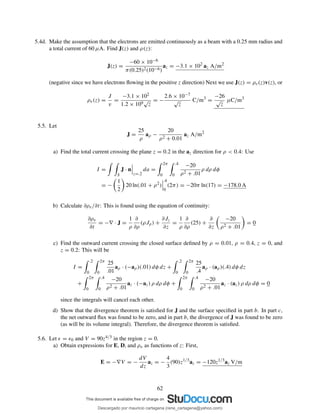
5.4. The cathode of a planar vacuum tube is at z = 0. Let E = −4 × 10⁶ az V/m for z > 0. An electron
(e = 1.602 × 10⁻¹⁹ C, m = 9.11 × 10⁻³¹ kg) is emitted from the cathode with zero initial velocity at
t = 0.
a) Find v(t): Using Newton’s second law, we write:
F = ma = qE ⇒ a =
(−1.602 × 10⁻¹⁹)(−4 × 10⁶)az
(9.11 × 10⁻³¹)
= 7.0 × 10¹⁷
az m/s2
Then v(t) = at = 7.0 × 10¹⁷t m/s.
b) Find z(t), the electron location as a function of time: Use
z(t) =
t
0
v(t′
)dt′
=
1
2
(7.0 × 10¹⁷
)t2
= 3.5 × 10¹⁷
t2
m
c) Determine v(z): Solve the result of part b for t, obtaining
t =
√
z
√
3.5 × 1017
= 1.7 × 10⁹√
z
Substitute into the result of part a to find v(z) = 7.0 × 10¹⁷(1.7 × 10⁻⁹)
√
z = 1.2 × 10⁹√
z m/s.
61
Descargado por mauricio cartagena (rene_cartagena@yahoo.com)
lOMoARcPSD|5423334](https://image.slidesharecdn.com/solucionario-teoria-electromagnetica-hayt-2001-201211183707/85/Solucionario-teoria-electromagnetica-hayt-2001-63-320.jpg)
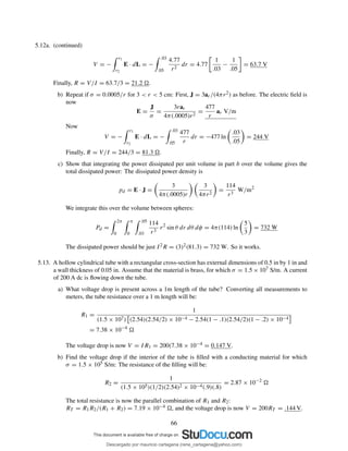
![5.9a. Using data tabulated in Appendix C, calculate the required diameter for a 2-m long nichrome wire that
will dissipate an average power of 450 W when 120 V rms at 60 Hz is applied to it:
The required resistance will be
R =
V 2
P
=
l
σ(πa2)
Thus the diameter will be
d = 2a = 2
lP
σπV 2
= 2
2(450)
(106)π(120)2
= 2.8 × 10⁻⁴
m = 0.28 mm
b) Calculate the rms current density in the wire: The rms current will be I = 450/120 = 3.75 A.
Thus
J =
3.75
π 2.8 × 10⁻⁴/2
2
= 6.0 × 10⁷
A/m2
5.10. A steel wire has a radius of 2 mm and a conductivity of 2 × 10⁶ S/m. The steel wire has an aluminum
(σ = 3.8 × 10⁷ S/m) coating of 2 mm thickness. Let the total current carried by this hybrid conductor
be 80 A dc. Find:
a) Jst . We begin with the fact that electric field must be the same in the aluminum and steel regions.
This comes from the requirement that E tangent to the boundary between two media must be
continuous, and from the fact that when integrating E over the wire length, the applied voltage
value must be obtained, regardless of the medium within which this integral is evaluated. We can
therefore write
EAl = Est =
JAl
σAl
=
Jst
σst
⇒ JAl =
σAl
σst
Jst
The net current is now expressed as the sum of the currents in each region, written as the sum of
the products of the current densities in each region times the appropriate cross-sectional area:
I = π(2 × 10⁻³
)2
Jst + π[(4 × 10⁻³
)2
− (2 × 10⁻³
)2
]JAl = 80 A
Using the above relation between Jst and JAl, we find
80 = π (2 × 10⁻³
)2
1 −
3.8 × 10⁷
6 × 10⁶
+ (4 × 10⁻³
)2 3.8 × 10⁷
6 × 10⁶
Jst
Solve for Jst to find Jst = 3.2 × 10⁵ A/m2.
b)
JAl =
3.8 × 10⁷
6 × 10⁶
(3.2 × 10⁵
) = 2.0 × 10⁶
A/m2
c,d) Est = EAl = Jst /σst = JAl/σAl = 5.3 × 10⁻² V/m.
e) the voltage between the ends of the conductor if it is 1 mi long: Using the fact that 1 mi = 1.61×10³
m, we have V = El = (5.3 × 10⁻²)(1.61 × 10³) = 85.4 V.
64
Descargado por mauricio cartagena (rene_cartagena@yahoo.com)
lOMoARcPSD|5423334](https://image.slidesharecdn.com/solucionario-teoria-electromagnetica-hayt-2001-201211183707/85/Solucionario-teoria-electromagnetica-hayt-2001-66-320.jpg)
![5.19b. (continued) Now
E = −∇V = −40xyz ax − 20x2
z ay − [20xy − 20z] az
Then, at the given point, we have
D(2, 7/8, 1) = ǫ0E(2, 7/8, 1) = −ǫ0[70 ax + 80 ay + 50 az] C/m2
We know that since this is the higher potential surface, D must be directed away from it, and so
the charge density would be positive. Thus
ρs =
√
D · D = 10ǫ0 72 + 82 + 52 = 1.04 nC/m2
c) Give the unit vector at this point that is normal to the conducting surface and directed toward the
V = 0 surface: This will be in the direction of E and D as found in part b, or
an = −
7ax + 8ay + 5az
√
72 + 82 + 52
= −[0.60ax + 0.68ay + 0.43az]
5.20. A conducting plane is located at z = 0 in free space, and a 20 nC point charge is present at Q(2, 4, 6).
a) If V = 0 at z = 0, find V at P (5, 3, 1): The plane can be replaced by an image charge of -20 nC
at Q′(2, 4, −6). Vectors R and R′ directed from Q and Q′ to P are R = (5, 3, 1) − (2, 4, 6) =
(3, −1, −5) and R′ = (5, 3, 1) − (2, 4, −6) = (3, −1, 7). Their magnitudes are R =
√
35 and
R′ =
√
59. The potential at P is given by
VP =
q
4πǫ0R
−
q
4πǫ0R′
=
20 × 10−9
4πǫ0
√
35
−
20 × 10−9
4πǫ0
√
59
= 7.0 V
b) Find E at P :
EP =
qR
4πǫ0R3
−
qR′
4πǫ0(R′)3
=
(20 × 10−9)(3, −1, −5)
4πǫ0(35)3/2
−
(20 × 10−9)(3, −1, 7)
4πǫ0(59)3/2
=
20 × 10−9
4πǫ0
(3ax − ay)
1
(35)3/2
−
1
(59)3/2
−
7
(59)3/2
+
5
(35)3/2
az
= 1.4ax − 0.47ay − 7.1az V/m
c) Find ρs at A(5, 3, 0): First, find the electric field there:
EA =
20 × 10−9
4πǫ0
(5, 3, 0) − (2, 4, 6)
(46)3/2
−
(5, 3, 0) − (2, 4, −6)
(46)3/2
= −6.9az V/m
Then ρs = D · n
surf ace
= −6.9ǫ0az · az = −61 pC/m2.
70
Descargado por mauricio cartagena (rene_cartagena@yahoo.com)
lOMoARcPSD|5423334](https://image.slidesharecdn.com/solucionario-teoria-electromagnetica-hayt-2001-201211183707/85/Solucionario-teoria-electromagnetica-hayt-2001-72-320.jpg)
![5.22b. Find |ρs| at B(0, 0, 0) (note error in problem statement): First, E at the origin is done as per the setup
in part a, except the vectors are directed from the charges to the origin:
EB =
10−9
4πǫ0
(4)(−7, −1, 2)
(54)3/2
−
(3)(−4, −2, −1)
(21)3/2
−
(4)(7, −1, 2)
(54)3/2
+
(3)(4, −2, −1)
(21)3/2
Now ρs = D · n|surf ace = D · ax in our case (note the other components cancel anyway as they must,
but we still need to express ρs as a scalar):
ρsB = ǫ0EB · ax =
10−9
4π
(4)(−7)
(54)3/2
−
(3)(−4)
(21)3/2
−
(4)(7)
(54)3/2
+
(3)(4)
(21)3/2
= 8.62 pC/m2
5.23. A dipole with p = 0.1az µC · m is located at A(1, 0, 0) in free space, and the x = 0 plane is perfectly-
conducting.
a) Find V at P (2, 0, 1). We use the far-field potential for a z-directed dipole:
V =
p cos θ
4πǫ0r2
=
p
4πǫ0
z
[x2 + y2 + z2]1.5
The dipole at x = 1 will image in the plane to produce a second dipole of the opposite orientation
at x = −1. The potential at any point is now:
V =
p
4πǫ0
z
[(x − 1)2 + y2 + z2]1.5
−
z
[(x + 1)2 + y2 + z2]1.5
Substituting P (2, 0, 1), we find
V =
.1 × 106
4πǫ0
1
2
√
2
−
1
10
√
10
= 289.5 V
b) Find the equation of the 200-V equipotential surface in cartesian coordinates: We just set the
potential exression of part a equal to 200 V to obtain:
z
[(x − 1)2 + y2 + z2]1.5
−
z
[(x + 1)2 + y2 + z2]1.5
= 0.222
5.24. The mobilities for intrinsic silicon at a certain temperature are µe = 0.14 m2/V · s and µh =
0.035 m2/V · s. The concentration of both holes and electrons is 2.2 × 10¹⁶ m−3. Determine both
the conductivity and the resistivity of this silicon sample: Use
σ = −ρeµe + ρhµh = (1.6 × 10⁻¹⁹
C)(2.2 × 10¹⁶
m−3
)(0.14 m2
/V · s + 0.035 m2
/V · s)
= 6.2 × 10⁻⁴
S/m
Conductivity is ρ = 1/σ = 1.6 × 10³ · m.
72
Descargado por mauricio cartagena (rene_cartagena@yahoo.com)
lOMoARcPSD|5423334](https://image.slidesharecdn.com/solucionario-teoria-electromagnetica-hayt-2001-201211183707/85/Solucionario-teoria-electromagnetica-hayt-2001-74-320.jpg)
![5.25. Electron and hole concentrations increase with temperature. For pure silicon, suitable expressions are
ρh = −ρe = 6200T 1.5e−7000/T C/m3. The functional dependence of the mobilities on temperature is
given by µh = 2.3 × 10⁵T −2.7 m2/V · s and µe = 2.1 × 10⁵T −2.5 m2/V · s, where the temperature,
T , is in degrees Kelvin. The conductivity will thus be
σ = −ρeµe + ρhµh = 6200T 1.5
e−7000/T
2.1 × 10⁵
T −2.5
+ 2.3 × 10⁵
T −2.7
=
1.30 × 10⁹
T
e−7000/T
1 + 1.095T −.2
S/m
Find σ at:
a) 0◦ C: With T = 273◦K, the expression evaluates as σ(0) = 4.7 × 10⁻⁵ S/m.
b) 40◦ C: With T = 273 + 40 = 313, we obtain σ(40) = 1.1 × 10⁻³ S/m.
c) 80◦ C: With T = 273 + 80 = 353, we obtain σ(80) = 1.2 × 10⁻² S/m.
5.26. A little donor impurity, such as arsenic, is added to pure silicon so that the electron concentration
is 2 × 10¹⁷ conduction electrons per cubic meter while the number of holes per cubic meter is only
1.1×10¹⁵. If µe = 0.15 m2/V · s for this sample, and µh = 0.045 m2/V · s, determine the conductivity
and resistivity:
σ = −ρeµe + ρhµh = (1.6 × 10⁻¹⁹
) (2 × 10¹⁷
)(0.15) + (1.1 × 10¹⁵
)(0.045) = 4.8 × 10⁻³
S/m
Then ρ = 1/σ = 2.1 × 10² · m.
5.27. Atomic hydrogen contains 5.5×1025 atoms/m3 at a certain temperature and pressure. When an electric
field of 4 kV/m is applied, each dipole formed by the electron and positive nucleus has an effective
length of 7.1 × 10⁻¹⁹ m.
a) Find P: With all identical dipoles, we have
P = Nqd = (5.5 × 1025
)(1.602 × 10⁻¹⁹
)(7.1 × 10⁻¹⁹
) = 6.26 × 10⁻¹²
C/m2
= 6.26 pC/m2
b) Find ǫR: We use P = ǫ0χeE, and so
χe =
P
ǫ0E
=
6.26 × 10⁻¹²
(8.85 × 10⁻¹²)(4 × 10³)
= 1.76 × 10⁻⁴
Then ǫR = 1 + χe = 1.000176.
5.28. In a certain region where the relative permittivity is 2.4, D = 2ax − 4ay + 5az nC/m2. Find:
a) E =
D
ǫ
=
(2ax − 4ay + 5az) × 10−9
(2.4)(8.85 × 10⁻¹²)
= 94ax − 188ay + 235az V/m
b) P = D − ǫ0E = ǫ0E(ǫR − 1) =
(2ax − 4ay + 5az) × 10−9
2.4
(2.4 − 1)
= 1.2ax − 2.3ay + 2.9az nC/m2
c) |∇V | = |E| = [(94.1)2
+ (188)2
+ (235)2
]1/2
= 315 V/m
73
Descargado por mauricio cartagena (rene_cartagena@yahoo.com)
lOMoARcPSD|5423334](https://image.slidesharecdn.com/solucionario-teoria-electromagnetica-hayt-2001-201211183707/85/Solucionario-teoria-electromagnetica-hayt-2001-75-320.jpg)
![5.31 (continued)
f) DN2 = DN1 = ǫR1ǫ0EN1 = 3(8.85 × 10⁻¹²)(80) = 2.12 nC/m2.
g) DT 2 = ǫR2ǫ0ET 1 = 5(8.85 × 10⁻¹²)(67.1) = 2.97 nC/m2.
h) D2 = ǫR1ǫ0EN1ax + ǫR2ǫ0ET 1 = 2.12ax − 2.66ay − 1.33az nC/m2.
i) P2 = D2 − ǫ0E2 = D2 [1 − (1/ǫR2)] = (4/5)D2 = 1.70ax − 2.13ay − 1.06az nC/m2.
j) the angle θ2 between E2 and a normal to the surface: Use
cos θ2 =
E2 · ax
E2
=
D2 · ax
D2
=
2.12
(2.12)2 = (2.66)2 + (1.33)2
= .581
Thus θ2 = cos−1(.581) = 54.5◦.
5.32. In Fig. 5.18, let D = 3ax − 4ay + 5az nC/m2 and find:
a) D2: First, the electric field in region 1 is
E1 =
3
2ǫ0
ax −
4
2ǫ0
ay +
5
2ǫ0
az × 10−9
V/m
Since, at the dielectric interface, tangential electric field and normal electric flux density are
continuous, we may write
D2 = ǫR2ǫ0ET 1 + DN1 =
5
2
3ax −
5
2
4ay + 5az = 7.5ax − 10ay + 5az nC/m2
b) DN2 = 5az, as explained above.
c) DT 2 = ǫR2ǫ0ET 2 = ǫR2ǫ0ET 1 = 7.5ax − 10ay nC/m2.
d) the energy density in each region:
we1 =
1
2
ǫR1ǫ0E1 · E1 =
1
2
(2)ǫ0
3
2ǫ0
2
+
4
2ǫ0
2
+
5
2ǫ0
2
× 10−18
= 1.41 µJ/m3
we2 =
1
2
ǫR2ǫ0E2 · E2 =
1
2
(5)ǫ0
3
2ǫ0
2
+
4
2ǫ0
2
+
5
5ǫ0
2
× 10−18
= 2.04 µJ/m3
e) the angle that D2 makes with az: Use D2 · az = |D2| cos θ = Dz = 5. where |D2| =
(7.5)2 + (10)2 + (5)2 1/2
= 13.5. So θ = cos−1(5/13.5) = 68◦.
f) D2/D1 = (7.5)2 + (10)2 + (5)2 1/2
/ (3)2 + (4)2 + (5)2 1/2
= 1.91.
g) P2/P1: First P1 = ǫ0E1(ǫR1 − 1) = 1.5ax − 2ay + 2.5az nC/m2.
Then P2 = ǫ0E2(ǫR2 − 1) = 6ax − 8ay + 4az nC/m2. So
P2
P1
=
[(6)2 + (8)2 + (4)2]1/2
[(1.5)2 + (2)2 + (2.5)2]1/2
= 3.04
75
Descargado por mauricio cartagena (rene_cartagena@yahoo.com)
lOMoARcPSD|5423334](https://image.slidesharecdn.com/solucionario-teoria-electromagnetica-hayt-2001-201211183707/85/Solucionario-teoria-electromagnetica-hayt-2001-77-320.jpg)
![5.33. Two perfect dielectrics have relative permittivities ǫR1 = 2 and ǫR2 = 8. The planar interface between
them is the surface x − y + 2z = 5. The origin lies in region 1. If E1 = 100ax + 200ay − 50az
V/m, find E2: We need to find the components of E1 that are normal and tangent to the boundary, and
then apply the appropriate boundary conditions. The normal component will be EN1 = E1 · n. Taking
f = x − y + 2z, the unit vector that is normal to the surface is
n =
∇f
|∇f |
=
1
√
6
ax − ay + 2az
This normal will point in the direction of increasing f , which will be away from the origin, or into region
2 (you can visualize a portion of the surface as a triangle whose vertices are on the three coordinate
axes at x = 5, y = −5, and z = 2.5). So EN1 = (1/
√
6)[100 − 200 − 100] = −81.7 V/m. Since the
magnitude is negative, the normal component points into region 1 from the surface. Then
EN1 = −81.65
1
√
6
[ax − ay + 2az] = −33.33ax + 33.33ay − 66.67az V/m
Now, the tangential component will be
ET 1 = E1 − EN1 = 133.3ax + 166.7ay + 16.67az
Our boundary conditions state that ET 2 = ET 1 and EN2 = (ǫR1/ǫR2)EN1 = (1/4)EN1. Thus
E2 = ET 2 + EN2 = ET 1 +
1
4
EN1 = 133.3ax + 166.7ay + 16.67az − 8.3ax + 8.3ay − 16.67az
= 125ax + 175ay V/m
5.34. Let the spherical surfaces r = 4 cm and r = 9 cm be separated by two perfect dielectric shells, ǫR1 = 2
for 4 < r < 6 cm and ǫR2 = 5 for 6 < r < 9 cm. If E1 = (2000/r2)ar V/m, find:
a) E2: Since E is normal to the interface between ǫR1 and ǫR2, D will be continuous across the
boundary, and so
D1 =
2ǫ0(2000)
r2
ar = D2
Then
E2 =
D2
5ǫ0
=
2
5
2000
r2
ar =
800
r2
ar V/m
b) the total electrostatic energy stored in each region: In region 1, the energy density is
we1 =
1
2
ǫR1ǫ0|E1|2
=
1
2
(2)ǫ0
(2000)2
r4
J/m3
In region 2:
we2 =
1
2
ǫR2ǫ0|E2|2
=
1
2
(5)ǫ0
(800)2
r4
J/m3
76
Descargado por mauricio cartagena (rene_cartagena@yahoo.com)
lOMoARcPSD|5423334](https://image.slidesharecdn.com/solucionario-teoria-electromagnetica-hayt-2001-201211183707/85/Solucionario-teoria-electromagnetica-hayt-2001-78-320.jpg)
![5.34. (continued)
The energies in each region are then
Region 1 : We1 = (2000)2
ǫ0
2π
0
π
0
.06
.04
1
r2
r2
sin θ dr dθ dφ
= 4πǫ0(2000)2 1
.04
−
1
.06
= 3.7 mJ
Region 2 : We2 = (800)2 5
2
ǫ0
2π
0
π
0
.09
.06
1
r2
r2
sin θ dr dθ dφ
= 4πǫ0(800)2 5
2
1
.06
−
1
.09
= 0.99 mJ
5.35. Let the cylindrical surfaces ρ = 4 cm and ρ = 9 cm enclose two wedges of perfect dielectrics, ǫR1 = 2
for 0 < φ < π/2, and ǫR2 = 5 for π/2 < φ < 2π. If E1 = (2000/ρ)aρ V/m, find:
a) E2: The interfaces between the two media will lie on planes of constant φ, to which E1 is parallel.
Thus the field is the same on either side of the boundaries, and so E2 = E1.
b) the total electrostatic energy stored in a 1m length of each region: In general we have wE =
(1/2)ǫRǫ0E2. So in region 1:
WE1 =
1
0
π/2
0
9
4
1
2
(2)ǫ0
(2000)2
ρ2
ρ dρ dφ dz =
π
2
ǫ0(2000)2
ln
9
4
= 45.1 µJ
In region 2, we have
WE2 =
1
0
2π
π/2
9
4
1
2
(5)ǫ0
(2000)2
ρ2
ρ dρ dφ dz =
15π
4
ǫ0(2000)2
ln
9
4
= 338 µJ
5.36. Let S = 120 cm2, d = 4 mm, and ǫR = 12 for a parallel-plate capacitor.
a) Calculate the capacitance:
C = ǫRǫ0S/d = [12ǫ0(120 × 10−4)]/[4 × 10−3] = 3.19 × 10−10 = 319 pF.
b) After connecting a 40 V battery across the capacitor, calculate E, D, Q, and the total stored
electrostatic energy: E = V/d = 40/(4 × 10−3) = 104 V/m. D = ǫRǫ0E = 12ǫ0 × 104 =
1.06 µC/m2. Then Q = D · n|surf ace × S = 1.06 × 10−6 × (120 × 10−4) = 1.27 × 10⁻⁸C =
12.7 nC. Finally We = (1/2)CV 2
0 = (1/2)(319 × 10−12)(40)2 = 255 nJ.
c) Thesourceisnowremovedandthedielectriciscarefullywithdrawnfrombetweentheplates. Again
calculate E, D, Q, and the energy: With the source disconnected, the charge is constant, and thus
so is D: Therefore, Q = 12.7 nC, D = 1.06 µC/m2, and E = D/ǫ0 = 104/8.85 × 10−12 =
1.2 × 10⁵ V/m. The energy is then
We =
1
2
D · E × S =
1
2
(1.06 × 10⁻⁶
)(1.2 × 10⁵
)(120 × 10−4
)(4 × 10⁻³
) = 3.05 µJ
d) What is the voltage between the plates? V = E × d = (1.2 × 10⁵)(4 × 10⁻³) = 480 V.
77
Descargado por mauricio cartagena (rene_cartagena@yahoo.com)
lOMoARcPSD|5423334](https://image.slidesharecdn.com/solucionario-teoria-electromagnetica-hayt-2001-201211183707/85/Solucionario-teoria-electromagnetica-hayt-2001-79-320.jpg)
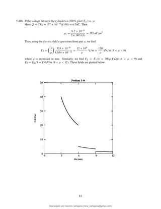
![5.48. A potential function in free space is given by
V = −20 + 10 ln
(5 + y)2 + x2
(5 − y)2 + x2
a) Describe the 0-V equipotential surface: Setting the given expression equal to zero, we find
(5 + y)2 + x2
(5 − y)2 + x2
= e2
= 7.39
So 6.39x2 + 6.39y2 − 83.9y + 160 = 0. Completing the square in the y trinomial leads to
x2 + (y − 6.56)2 = 18.1 = (4.25)2, which we recognize as a right circular cylinder whose axis
is located at x = 0, y = 6.56, and whose radius is 4.25.
b) Describe the 10-V equipotential surface: In this case, the given expression is set equal to ten,
leading to
(5 + y)2 + x2
(5 − y)2 + x2
= e3
= 20.1
So 19.1x2 + 19.1y2 − 211y + 477 = 0. Following the same procedure as in part a, this becomes
x2 + (y − 5.52)2 = 5.51 = (2.35)2, which we recognize again as a right circular cylinder with
axis at x = 0, y = 5.52, and of radius 2.35.
5.49. A 2 cm diameter conductor is suspended in air with its axis 5 cm from a conducting plane. Let the
potential of the cylinder be 100 V and that of the plane be 0 V. Find the surface charge density on the:
a) cylinder at a point nearest the plane: The cylinder will image across the plane, producing an
equivalent two-cylinder problem, with the second one at location 5 cm below the plane. We will
take the plane as the zy plane, with the cylinder positions at x = ±5. Now b = 1 cm, h = 5
cm, and V0 = 100 V. Thus a =
√
h2 − b2 = 4.90 cm. Then K1 = [(h + a)/b]2 = 98.0, and
ρL = (4πǫ0V0)/ ln K1 = 2.43 nC/m. Now
D = ǫ0E = −
ρL
2π
(x + a)ax + yay
(x + a)2 + y2
−
(x − a)ax + yay
(x − a)2 + y2
and
ρs, max = D · (−ax)
x=h−b,y=0
=
ρL
2π
h − b + a
(h − b + a)2
−
h − b − a
(h − b − a)2
= 473 nC/m2
b) plane at a point nearest the cylinder: At x = y = 0,
D(0, 0) = −
ρL
2π
aax
a2
−
−aax
a2
= −
ρL
2π
2
a
ax
from which
ρs = D(0, 0) · ax = −
ρL
πa
= −15.8 nC/m2
83
Descargado por mauricio cartagena (rene_cartagena@yahoo.com)
lOMoARcPSD|5423334](https://image.slidesharecdn.com/solucionario-teoria-electromagnetica-hayt-2001-201211183707/85/Solucionario-teoria-electromagnetica-hayt-2001-85-320.jpg)
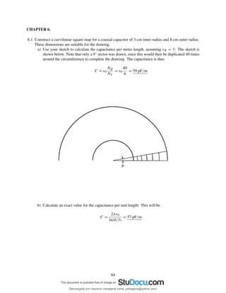
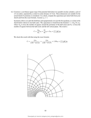
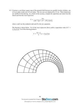
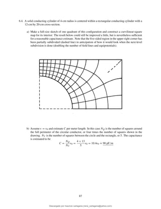
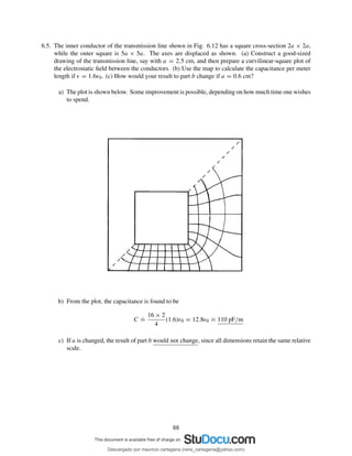
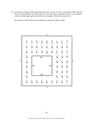
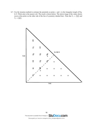
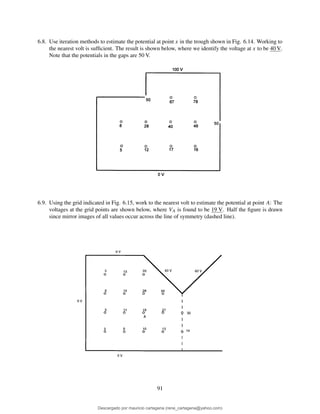
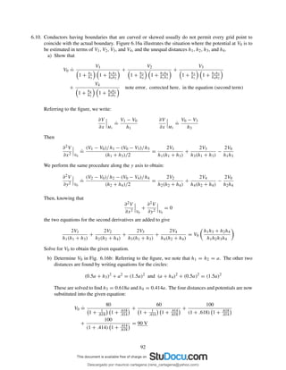
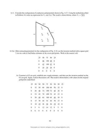
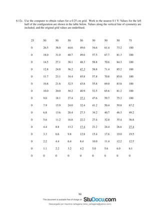
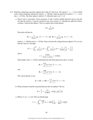
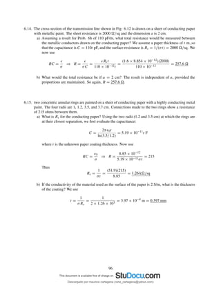
![6.16. The square washer shown in Fig. 6.19 is 2.4 mm thick and has outer dimensions of 2.5 × 2.5 cm
and inner dimensions of 1.25 × 1.25 cm. The inside and outside surfaces are perfectly-conducting. If
the material has a conductivity of 6 S/m, estimate the resistance offered between the inner and outer
surfaces (shown shaded in Fig. 6.19). A few curvilinear squares are suggested: First we find the surface
resistance, Rs = 1/(σt) = 1/(6 × 2.4 × 10−3) = 69.4 /sq. Having found this, we can construct
the total resistance by using the fundamental square as a building block. Specifically, R = Rs(Nl/Nw)
where Nl is the number of squares between the inner and outer surfaces and Nw is the number of squares
around the perimeter of the washer. These numbers are found from the curvilinear square plot shown
below, which covers one-eighth the washer. The resistance is thus R
.
= 69.4[4/(8 × 5)]
.
= 6.9 .
6.17. A two-wire transmission line consists of two parallel perfectly-conducting cylinders, each having a
radius of 0.2 mm, separated by center-to-center distance of 2 mm. The medium surrounding the wires
has ǫR = 3 and σ = 1.5 mS/m. A 100-V battery is connected between the wires. Calculate:
a) the magnitude of the charge per meter length on each wire: Use
C =
πǫ
cosh−1(h/b)
=
π × 3 × 8.85 × 10−12
cosh−1 (1/0.2)
= 3.64 × 10⁻⁹
C/m
Then the charge per unit length will be
Q = CV0 = (3.64 × 10⁻¹¹
)(100) = 3.64 × 10⁻⁹
C/m = 3.64 nC/m
b) the battery current: Use
RC =
ǫ
σ
⇒ R =
3 × 8.85 × 10−12
(1.5 × 10⁻³)(3.64 × 10⁻¹¹)
= 486
Then
I =
V0
R
=
100
486
= 0.206 A = 206 mA
97
Descargado por mauricio cartagena (rene_cartagena@yahoo.com)
lOMoARcPSD|5423334](https://image.slidesharecdn.com/solucionario-teoria-electromagnetica-hayt-2001-201211183707/85/Solucionario-teoria-electromagnetica-hayt-2001-99-320.jpg)
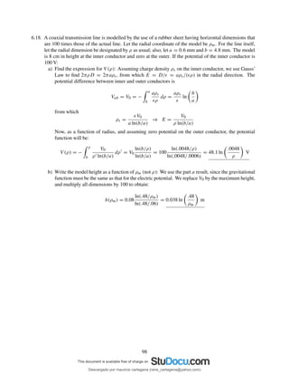
![7.22c. Use a development similar to that of Sec. 7.4 to show that C = dQ/dV0 = ǫS/8a ( note error in
problem statement): First, the overall potential difference is
V0 = Vx→∞ − Vx→−∞ = 2 ×
2a2ρv0
ǫ
=
4a2ρv0
ǫ
From this we find a =
√
(ǫV0)/(4ρv0). Then the total charge on one side will be
Q = S
∞
0
ρv0
x
a
e−x/a
dx = Sρv0 ae−x/a −x
a
− 1
∞
0
= Sρv0 a =
1
2
S ǫV0ρv0
Now
C =
dQ
dV0
=
d
dV0
1
2
S ǫV0ρv0 =
S
4
ρv0 ǫ
V0
But a =
√
(ǫV0)/(4ρv0), from which (ρv0/V0) = ǫ/(4a2). Substituting this into the capacitance
expression gives
C =
S
4
ǫ2
4a2
=
ǫS
8a
7.23. A rectangular trough is formed by four conducting planes located at x = 0 and 8 cm and y = 0 and 5
cm in air. The surface at y = 5 cm is at a potential of 100 V, the other three are at zero potential, and the
necessary gaps are placed at two corners. Find the potential at x = 3 cm, y = 4 cm: This situation is
the same as that of Fig. 7.6, except the non-zero boundary potential appears on the top surface, rather
than the right side. The solution is found from Eq. (39) by simply interchanging x and y, and b and d,
obtaining:
V (x, y) =
4V0
π
∞
1,odd
1
m
sinh(mπy/d)
sinh(mπb/d)
sin
mπx
d
where V0 = 100 V, d = 8 cm, and b = 5 cm. We will use the first three terms to evaluate the potential
at (3,4):
V (3, 4)
.
=
400
π
sinh(π/2)
sinh(5π/8)
sin(3π/8) +
1
3
sinh(3π/2)
sinh(15π/8)
sin(9π/8) +
1
5
sinh(5π/2)
sinh(25π/8)
sin(15π/8)
=
400
π
[.609 − .040 − .011] = 71.1 V
Additional accuracy is found by including more terms in the expansion. Using thirteen terms, and
using six significant figure accuracy, the result becomes V (3, 4)
.
= 71.9173 V. The series converges
rapidly enough so that terms after the sixth one produce no change in the third digit. Thus, quoting
three significant figures, 71.9 V requires six terms, with subsequent terms having no effect.
111
Descargado por mauricio cartagena (rene_cartagena@yahoo.com)
lOMoARcPSD|5423334](https://image.slidesharecdn.com/solucionario-teoria-electromagnetica-hayt-2001-201211183707/85/Solucionario-teoria-electromagnetica-hayt-2001-113-320.jpg)
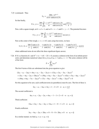
![7.28b. Show that P = Aρn + Bρ−n satisfies the ρ equation: From part a, the radial equation is:
ρ2 d2P
dρ2
+ ρ
dP
dρ
− n2
P = 0
Substituting Aρn, we find
ρ2
n(n − 1)ρn−2
+ ρnρn−1
− n2
ρn
= n2
ρn
− nρn
+ nρn
− n2
ρn
= 0
Substituting Bρ−n:
ρ2
n(n + 1)ρ−(n+2)
− ρnρ−(n+1)
− n2
ρ−n
= n2
ρ−n
+ nρ−n
− nρ−n
− n2
ρ−n
= 0
So it works.
c) Construct the solution V (ρ, φ). Functions of this form are called circular harmonics. To assemble
the complete solution, we need the radial solution for the case in which n = 0. The equation to
solve is
ρ
d2P
dρ2
+
dP
dρ
= 0
Let S = dP/dρ, and so dS/dρ = d2P/dρ2. The equation becomes
ρ
dS
dρ
+ S = 0 ⇒ −
dρ
ρ
=
dS
S
Integrating, find
− ln ρ + ln A0 = ln S ⇒ ln S = ln
A0
ρ
⇒ S =
A0
ρ
=
dP
dρ
where A0 is a constant. So now
dρ
ρ
=
dP
A0
⇒ Pn=0 = A0 ln ρ + B0
We may now construct the solution in its complete form, encompassing n ≥ 0:
V (ρ, φ) = (A0 ln ρ + B0)(C0φ + D0)
n=0 solution
+
∞
n=1
[Anρn
+ Bnρ−n
][Cn cos(nφ) + Dn sin(nφ)]
115
Descargado por mauricio cartagena (rene_cartagena@yahoo.com)
lOMoARcPSD|5423334](https://image.slidesharecdn.com/solucionario-teoria-electromagnetica-hayt-2001-201211183707/85/Solucionario-teoria-electromagnetica-hayt-2001-117-320.jpg)
![CHAPTER 8
8.1a. Find H in cartesian components at P (2, 3, 4) if there is a current filament on the z axis carrying 8 mA
in the az direction:
Applying the Biot-Savart Law, we obtain
Ha =
∞
−∞
IdL × aR
4πR2
=
∞
−∞
Idz az × [2ax + 3ay + (4 − z)az]
4π(z2 − 8z + 29)3/2
=
∞
−∞
Idz[2ay − 3ax]
4π(z2 − 8z + 29)3/2
Using integral tables, this evaluates as
Ha =
I
4π
2(2z − 8)(2ay − 3ax)
52(z2 − 8z + 29)1/2
∞
−∞
=
I
26π
(2ay − 3ax)
Then with I = 8 mA, we finally obtain Ha = −294ax + 196ay µA/m
b. Repeat if the filament is located at x = −1, y = 2: In this case the Biot-Savart integral becomes
Hb =
∞
−∞
Idz az × [(2 + 1)ax + (3 − 2)ay + (4 − z)az]
4π(z2 − 8z + 26)3/2
=
∞
−∞
Idz[3ay − ax]
4π(z2 − 8z + 26)3/2
Evaluating as before, we obtain with I = 8 mA:
Hb =
I
4π
2(2z − 8)(3ay − ax)
40(z2 − 8z + 26)1/2
∞
−∞
=
I
20π
(3ay − ax) = −127ax + 382ay µA/m
c. Find H if both filaments are present: This will be just the sum of the results of parts a and b, or
HT = Ha + Hb = −421ax + 578ay µA/m
This problem can also be done (somewhat more simply) by using the known result for H from an
infinitely-long wire in cylindrical components, and transforming to cartesian components. The Biot-
Savart method was used here for the sake of illustration.
8.2. A current filament of 3ax A lies along the x axis. Find H in cartesian components at P (−1, 3, 2): We
use the Biot-Savart law,
H =
IdL × aR
4πR2
where IdL = 3dxax, aR = [−(1 + x)ax + 3ay + 2az]/R, and R =
√
x2 + 2x + 14. Thus
HP =
∞
−∞
3dxax × [−(1 + x)ax + 3ay + 2az]
4π(x2 + 2x + 14)3/2
=
∞
−∞
(9az − 6ay) dx
4π(x2 + 2x + 14)3/2
=
(9az − 6ay)(x + 1)
4π(13)
√
x2 + 2x + 14
∞
−∞
=
2(9az − 6ay)
4π(13)
= 0.110az − 0.073ay A/m
116
Descargado por mauricio cartagena (rene_cartagena@yahoo.com)
lOMoARcPSD|5423334](https://image.slidesharecdn.com/solucionario-teoria-electromagnetica-hayt-2001-201211183707/85/Solucionario-teoria-electromagnetica-hayt-2001-118-320.jpg)
![8.3. Two semi-infinite filaments on the z axis lie in the regions −∞ < z < −a (note typographical error in
problem statement) and a < z < ∞. Each carries a current I in the az direction.
a) Calculate H as a function of ρ and φ at z = 0: One way to do this is to use the field from an
infinite line and subtract from it that portion of the field that would arise from the current segment
at −a < z < a, found from the Biot-Savart law. Thus,
H =
I
2πρ
aφ −
a
−a
I dz az × [ρ aρ − z az]
4π[ρ2 + z2]3/2
The integral part simplifies and is evaluated:
a
−a
I dz ρ aφ
4π[ρ2 + z2]3/2
=
Iρ
4π
aφ
z
ρ2 ρ2 + z2
a
−a
=
Ia
2πρ ρ2 + a2
aφ
Finally,
H =
I
2πρ
1 −
a
ρ2 + a2
aφ A/m
b) What value of a will cause the magnitude of H at ρ = 1, z = 0, to be one-half the value obtained
for an infinite filament? We require
1 −
a
ρ2 + a2
ρ=1
=
1
2
⇒
a
√
1 + a2
=
1
2
⇒ a = 1/
√
3
8.4a.) A filament is formed into a circle of radius a, centered at the origin in the plane z = 0. It carries a
current I in the aφ direction. Find H at the origin: We use the Biot-Savart law, which in this case
becomes:
H =
loop
IdL × aR
4πR2
=
2π
0
Ia dφ aφ × (−aρ)
4πa2
= 0.50
I
a
az A/m
b.) A filament of the same length is shaped into a square in the z = 0 plane. The sides are parallel to the
coordinate axes and a current I flows in the general aφ direction. Again, find H at the origin: Since
the loop is the same length, its perimeter is 2πa, and so each of the four sides is of length πa/2.
Using symmetry, we can find the magnetic field at the origin associated with each of the 8 half-sides
(extending from 0 to ±πa/4 along each coordinate direction) and multiply the result by 8: Taking one
of the segments in the y direction, the Biot-Savart law becomes
H =
loop
IdL × aR
4πR2
= 8
πa/4
0
Idy ay × −(πa/4) ax − y ay
4π y2 + (πa/4)2 3/2
=
aI
2
πa/4
0
dy az
y2 + (πa/4)2 3/2
=
aI
2
y az
(πa/4)2 y2 + (πa/4)2
πa/4
0
= 0.57
I
a
az A/m
117
Descargado por mauricio cartagena (rene_cartagena@yahoo.com)
lOMoARcPSD|5423334](https://image.slidesharecdn.com/solucionario-teoria-electromagnetica-hayt-2001-201211183707/85/Solucionario-teoria-electromagnetica-hayt-2001-119-320.jpg)
![8.5. The parallel filamentary conductors shown in Fig. 8.21 lie in free space. Plot |H| versus y, −4 < y < 4,
along the line x = 0, z = 2: We need an expression for H in cartesian coordinates. We can start with the
known H in cylindrical for an infinite filament along the z axis: H = I/(2πρ) aφ, which we transform
to cartesian to obtain:
H =
−Iy
2π(x2 + y2)
ax +
Ix
2π(x2 + y2)
ay
If we now rotate the filament so that it lies along the x axis, with current flowing in positive x, we obtain
the field from the above expression by replacing x with y and y with z:
H =
−Iz
2π(y2 + z2)
ay +
Iy
2π(y2 + z2)
az
Now, with two filaments, displaced from the x axis to lie at y = ±1, and with the current directions as
shown in the figure, we use the previous expression to write
H =
Iz
2π[(y + 1)2 + z2]
−
Iz
2π[(y − 1)2 + z2]
ay +
I(y − 1)
2π[(y − 1)2 + z2]
−
I(y + 1)
2π[(y + 1)2 + z2]
az
We now evaluate this at z = 2, and find the magnitude (
√
H · H), resulting in
|H| =
I
2π
2
y2 + 2y + 5
−
2
y2 − 2y + 5
2
+
(y − 1)
y2 − 2y + 5
−
(y + 1)
y2 + 2y + 5
2 1/2
This function is plotted below
8.6a. A current filament I is formed into circle, ρ = a, in the z = z′ plane. Find Hz at P (0, 0, z) if I flows
in the aφ direction: Use the Biot-Savart law,
H =
IdL × aR
4πR2
where in this case IdL = Idφaφ, aR = [−aaρ + (z − z′)az]/R, and R = a2 + (z − z′)2. The
setup becomes
H =
2π
0
Iadφ aφ × [−aaρ + (z − z′)az]
4π[a2 + (z − z′)2]3/2
=
2π
0
Ia[aaz + (z − z′)aρ] dφ
4π[a2 + (z − z′)2]3/2
118
Descargado por mauricio cartagena (rene_cartagena@yahoo.com)
lOMoARcPSD|5423334](https://image.slidesharecdn.com/solucionario-teoria-electromagnetica-hayt-2001-201211183707/85/Solucionario-teoria-electromagnetica-hayt-2001-120-320.jpg)
![At this point we need to be especially careful. Note that we are integrating a vector with an aρ component
around a complete circle, where the vector has no φ dependence. This sum of all aρ components will be
zero – even though this doesn’t happen when we go ahead with the integration without this knowledge.
The problem is that the integral “interprets” aρ as a constant direction, when in fact – as we know – aρ
continually changes direction as φ varies. We drop the aρ component in the integral to give
H =
2π
0
Ia2az dφ
4π[a2 + (z − z′)2]3/2
=
πa2Iaz
2π[a2 + (z − z′)2]3/2
=
m
2π[a2 + (z − z′)2]3/2
A/m
where m = πa2Iaz is the magnetic moment of the loop.
b) Find Hz at P caused by a uniform surface current density K = K0aφ, flowing on the cylindrical
surface, ρ = a, 0 < z < h. The results of part a should help: Using part a, we can write down the
differential field at P arising from a circular current ribbon of differential height, dz′, at location
z′. The ribbon is of radius a and carries current K0dz′aφ A:
dH =
πa2K0dz′az
2π[a2 + (z − z′)2]3/2
A/m
The total magnetic field at P is now the sum of the contributions of all differential rings that
comprise the cylinder:
Hz =
h
0
πa2K0dz′
2π[a2 + (z − z′)2]3/2
=
a2K0
2
h
0
dz′
[a2 + z2 − 2zz′ + (z′)2]3/2
=
a2K0
2
2(2z′ − 2z)
4a2 a2 + z2 − 2zz′ + (z′)2
h
0
=
K0(z′ − z)
2 a2 + (z′ − z)2
h
0
=
K0
2
(h − z)
a2 + (h − z)2
+
z
√
a2 + z2
A/m
8.7. Given points C(5, −2, 3) and P (4, −1, 2); a current element IdL = 10−4(4, −3, 1) A · m at C pro-
duces a field dH at P .
a) Specify the direction of dH by a unit vector aH : Using the Biot-Savart law, we find
dH =
IdL × aCP
4πR2
CP
=
10−4[4ax − 3ay + az] × [−ax + ay − az]
4π33/2
=
[2ax + 3ay + az] × 10−4
65.3
from which
aH =
2ax + 3ay + az
√
14
= 0.53ax + 0.80ay + 0.27az
b) Find |dH|.
|dH| =
√
14 × 10−4
65.3
= 5.73 × 10⁻⁶
A/m = 5.73 µA/m
c) What direction al should IdL have at C so that dH = 0? IdL should be collinear with aCP ,
thus rendering the cross product in the Biot-Savart law equal to zero. Thus the answer is al =
±(−ax + ay − az)/
√
3
119
Descargado por mauricio cartagena (rene_cartagena@yahoo.com)
lOMoARcPSD|5423334](https://image.slidesharecdn.com/solucionario-teoria-electromagnetica-hayt-2001-201211183707/85/Solucionario-teoria-electromagnetica-hayt-2001-121-320.jpg)
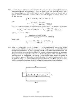
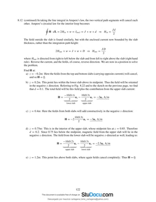
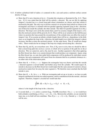
![8.14. A toroid having a cross section of rectangular shape is defined by the following surfaces: the cylinders
ρ = 2 and ρ = 3 cm, and the planes z = 1 and z = 2.5 cm. The toroid carries a surface current density
of −50az A/m on the surface ρ = 3 cm. Find H at the point P (ρ, φ, z): The construction is similar
to that of the toroid of round cross section as done on p.239. Again, magnetic field exists only inside
the toroid cross section, and is given by
H =
Iencl
2πρ
aφ (2 < ρ < 3) cm, (1 < z < 2.5) cm
where Iencl is found from the given current density: On the outer radius, the current is
Iouter = −50(2π × 3 × 10−2
) = −3π A
This current is directed along negative z, which means that the current on the inner radius (ρ = 2) is
directed along positive z. Inner and outer currents have the same magnitude. It is the inner current that
is enclosed by the circular integration path in aφ within the toroid that is used in Ampere’s law. So
Iencl = +3π A. We can now proceed with what is requested:
a) PA(1.5cm, 0, 2cm): The radius, ρ = 1.5 cm, lies outside the cross section, and so HA = 0.
b) PB(2.1cm, 0, 2cm): This point does lie inside the cross section, and the φ and z values do not
matter. We find
HB =
Iencl
2πρ
aφ =
3aφ
2(2.1 × 10⁻²)
= 71.4 aφ A/m
c) PC(2.7cm, π/2, 2cm): again, φ and z values make no difference, so
HC =
3aφ
2(2.7 × 10⁻²)
= 55.6 aφ A/m
d) PD(3.5cm, π/2, 2cm). This point lies outside the cross section, and so HD = 0.
8.15. Assume that there is a region with cylindrical symmetry in which the conductivity is given by σ =
1.5e−150ρ kS/m. An electric field of 30 az V/m is present.
a) Find J: Use
J = σE = 45e−150ρ
az kA/m2
b) Find the total current crossing the surface ρ < ρ0, z = 0, all φ:
I = J · dS =
2π
0
ρ0
0
45e−150ρ
ρ dρ dφ =
2π(45)
(150)2
e−150ρ
[−150ρ − 1]
ρ0
0
kA
= 12.6 1 − (1 + 150ρ0)e−150ρ0 A
c) Make use of Ampere’s circuital law to find H: Symmetry suggests that H will be φ-directed only,
and so we consider a circular path of integration, centered on and perpendicular to the z axis.
Ampere’s law becomes: 2πρHφ = Iencl, where Iencl is the current found in part b, except with ρ0
replaced by the variable, ρ. We obtain
Hφ =
2.00
ρ
1 − (1 + 150ρ)e−150ρ
A/m
124
Descargado por mauricio cartagena (rene_cartagena@yahoo.com)
lOMoARcPSD|5423334](https://image.slidesharecdn.com/solucionario-teoria-electromagnetica-hayt-2001-201211183707/85/Solucionario-teoria-electromagnetica-hayt-2001-126-320.jpg)
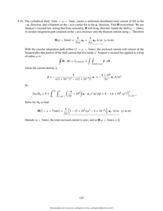
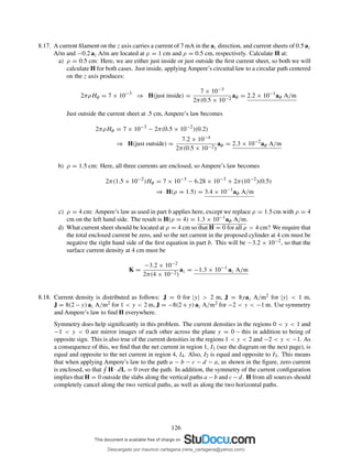
![8.18. (continued) To find the magnetic field in region 1, we apply Ampere’s circuital law to the path c −
d − e − f − c, again noting that H will be zero along the two horizontal segments and along the right
vertical segment. This leaves only the left vertical segment, e − f , pointing in the +x direction, and
along which is field, Hx1. The counter-clockwise direction of the path integral is chosen using the
right-hand convention, where we take the normal to the path in the +z direction, which is the same as
the current direction. Assuming the height of the path is x, we find
Hx1 x = x
2
y1
8(2 − y)dy = x 16y − 4y2
2
y1
= x 16(2 − y1) − 4(4 − y2
1)
Replacing y1 with y, we find
Hx1 = 4[8 − 4y − 4 + y2
] ⇒ H1(1 < y < 2) = 4(y − 2)2
ax A/m
H1 lies in the positive x direction, since the result of the integration is net positive.
H in region 2 is now found through the line integral over the path d − g − h − c, enclosing all of region
1 within x and part of region 2 from y = y2 to 1:
Hx2 x = x
2
1
8(2 − y) dy + x
1
y2
8y dy = x 4(1 − 2)2
+ 4(1 − y2
2) = 4(2 − y2
2) x
so that in terms of y,
H2(0 < y < 1) = 4(2 − y2
)ax A/m
y
x
1 20-1-2
a
b c
d
e
f
g
h
x x . .
I1I2I3I4
4 3 2 1
y2 y1
127
Descargado por mauricio cartagena (rene_cartagena@yahoo.com)
lOMoARcPSD|5423334](https://image.slidesharecdn.com/solucionario-teoria-electromagnetica-hayt-2001-201211183707/85/Solucionario-teoria-electromagnetica-hayt-2001-129-320.jpg)
![8.18. (continued) The procedure is repeated for the remaining two regions, −2 < y < −1 and −1 < y < 0,
by taking the integration path with its right vertical segment within each of these two regions, while
the left vertical path is a − b. Again the integral is taken counter-clockwise, which means that the
right vertical path will be directed along −x. But the current is now in the opposite direction of that
for y > 0, making the enclosed current net negative. Therefore, H will be in the opposite direction
from that of the right vertical path, which is the positive x direction. The magnetic field will therefore
be symmetric about the y = 0 plane. We can use the results for regions 1 and 2 to construct the field
everywhere:
H = 0 (y > 2) and (y < −2)
H = 4(2 − |y|2
)ax A/m (0 < |y| < 1)
H = 4(|y| − 2)2
ax A/m (1 < |y| < 2)
8.19. Calculate ∇ × [∇(∇ · G)] if G = 2x2yz ax − 20y ay + (x2 − z2) az: Proceding, we first find ∇ · G =
4xyz − 20 − 2z. Then ∇(∇ · G) = 4yz ax + 4xz ay + (4xy − 2) az. Then
∇ × [∇(∇ · G)] = (4x − 4x) ax − (4y − 4y) ay + (4z − 4z) az = 0
8.20. The magnetic field intensity is given in the square region x = 0, 0.5 < y < 1, 1 < z < 1.5 by
H = z2ax + x3ay + y4az A/m.
a) evaluate H · dL about the perimeter of the square region: Using dL = dxax + dyay + dzaz,
and using the given field, we find, in the x = 0 plane:
H · dL =
1
.5
0 dy +
1.5
1
(1)4
dz +
.5
1
0 dy +
1
1.5
(.5)4
dz = 0.46875
b) Find ∇ × H:
∇ × H =
∂Hz
∂y
−
∂Hy
∂z
ax +
∂Hx
∂z
−
∂Hz
∂x
ay +
∂Hy
∂x
−
∂Hx
∂y
az
= 4y3
ax + 2zay + 3x2
az
c) Calculate (∇ × H)x at the center of the region: Here, y = 0.75 and so (∇ × H)x = 4(.75)3 =
1.68750.
d) Does (∇×H)x = [ H·dL]/Area Enclosed? Using the part a result, [ H·dL]/Area Enclosed =
0.46875/0.25 = 1.8750, which is off the value found in part c. Answer: No. Reason: the limit
of the area shrinking to zero must be taken before the results will be equal.
8.21. Points A, B, C, D, E, and F are each 2 mm from the origin on the coordinate axes indicated in Fig.
8.23. The value of H at each point is given. Calculate an approximate value for ∇ × H at the origin:
We use the approximation:
curl H
.
=
H · dL
a
where no limit as a → 0 is taken (hence the approximation), and where a = 4 mm2. Each curl
component is found by integrating H over a square path that is normal to the component in question.
128
Descargado por mauricio cartagena (rene_cartagena@yahoo.com)
lOMoARcPSD|5423334](https://image.slidesharecdn.com/solucionario-teoria-electromagnetica-hayt-2001-201211183707/85/Solucionario-teoria-electromagnetica-hayt-2001-130-320.jpg)
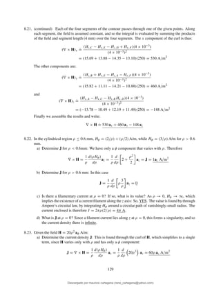
![8.23. (continued)
b) Integrate J over the circular surface ρ = 1, 0 < φ < 2π, z = 0, to determine the total current
passing through that surface in the az direction: The integral is:
I = J · dS =
2π
0
1
0
60ρaz · ρ dρ dφaz = 40π A
c) Find the total current once more, this time by a line integral around the circular path ρ = 1,
0 < φ < 2π, z = 0:
I = H · dL =
2π
0
20ρ2
aφ ρ=1
· (1)dφaφ =
2π
0
20 dφ = 40π A
8.24. Evaluate both sides of Stokes’theorem for the field G = 10 sin θ aφ and the surface r = 3, 0 ≤ θ ≤ 90◦,
0 ≤ φ ≤ 90◦. Let the surface have the ar direction: Stokes’ theorem reads:
C
G · dL =
S
(∇ × G) · n da
Considering the given surface, the contour, C, that forms its perimeter consists of three joined arcs of
radius 3 that sweep out 90◦ in the xy, xz, and zy planes. Their centers are at the origin. Of these three,
only the arc in the xy plane (which lies along aφ) is in the direction of G; the other two (in the −aθ and
aθ directions respectively) are perpendicular to it, and so will not contribute to the path integral. The
left-hand side therefore consists of only the xy plane portion of the closed path, and evaluates as
G · dL =
π/2
0
10 sin θ π/2
aφ · aφ 3 sin θ π/2
dφ = 15π
To evaluate the right-hand side, we first find
∇ × G =
1
r sin θ
d
dθ
[(sin θ)10 sin θ] ar =
20 cos θ
r
ar
The surface over which we integrate this is the one-eighth spherical shell of radius 3 in the first octant,
bounded by the three arcs described earlier. The right-hand side becomes
S
(∇ × G) · n da =
π/2
0
π/2
0
20 cos θ
3
ar · ar (3)2
sin θ dθ dφ = 15π
It would appear that the theorem works.
130
Descargado por mauricio cartagena (rene_cartagena@yahoo.com)
lOMoARcPSD|5423334](https://image.slidesharecdn.com/solucionario-teoria-electromagnetica-hayt-2001-201211183707/85/Solucionario-teoria-electromagnetica-hayt-2001-132-320.jpg)
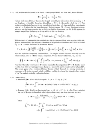
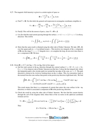
![8.30. A solid nonmagnetic conductor of circular cross-section has a radius of 2mm. The conductor is inho-
mogeneous, with σ = 106(1 + 106ρ2) S/m. If the conductor is 1m in length and has a voltage of 1mV
between its ends, find:
a) H inside: With current along the cylinder length (along az, and with φ symmetry, H will be φ-
directed only. We find E = (V0/d)az = 10−3az V/m. Then J = σE = 103(1 + 106ρ2)az A/m2.
Next we apply Ampere’s circuital law to a circular path of radius ρ, centered on the z axis and
normal to the axis:
H · dL = 2πρHφ =
S
J · dS =
2π
0
ρ
0
103
(1 + 106
(ρ′
)2
)az · azρ′
dρ′
dφ
Thus
Hφ =
103
ρ
ρ
0
ρ′
+ 106
(ρ′
)3
dρ′
=
103
ρ
ρ2
2
+
106
4
ρ4
Finally, H = 500ρ(1 + 5 × 10⁵ρ3)aφ A/m (0 < ρ < 2mm).
b) the total magnetic flux inside the conductor: With field in the φ direction, a plane normal to B will
be that in the region 0 < ρ < 2 mm, 0 < z < 1 m. The flux will be
=
S
B·dS = µ0
1
0
2×10⁻³
0
500ρ + 2.5 × 10⁸
ρ3
dρdz = 8π ×10−10
Wb = 2.5 nWb
8.31. The cylindrical shell defined by 1 cm < ρ < 1.4 cm consists of a non-magnetic conducting material
and carries a total current of 50 A in the az direction. Find the total magnetic flux crossing the plane
φ = 0, 0 < z < 1:
a) 0 < ρ < 1.2 cm: We first need to find J, H, and B: The current density will be:
J =
50
π[(1.4 × 10⁻²)2 − (1.0 × 10⁻²)2]
az = 1.66 × 10⁵
az A/m2
Next we find Hφ at radius ρ between 1.0 and 1.4 cm, by applying Ampere’s circuital law, and
noting that the current density is zero at radii less than 1 cm:
2πρHφ = Iencl =
2π
0
ρ
10−2
1.66 × 10⁵
ρ′
dρ′
dφ
⇒ Hφ = 8.30 × 10⁴ (ρ2 − 10−4)
ρ
A/m (10−2
m < ρ < 1.4 × 10⁻²
m)
Then B = µ0H, or
B = 0.104
(ρ2 − 10−4)
ρ
aφ Wb/m2
Now,
a = B · dS =
1
0
1.2×10⁻²
10−2
0.104 ρ −
10−4
ρ
dρ dz
= 0.104
(1.2 × 10⁻²)2 − 10−4
2
− 10−4
ln
1.2
1.0
= 3.92 × 10⁻⁷
Wb = 0.392 µWb
134
Descargado por mauricio cartagena (rene_cartagena@yahoo.com)
lOMoARcPSD|5423334](https://image.slidesharecdn.com/solucionario-teoria-electromagnetica-hayt-2001-201211183707/85/Solucionario-teoria-electromagnetica-hayt-2001-136-320.jpg)
![8.31b) 1.0 cm < ρ < 1.4 cm (note typo in book): This is part a over again, except we change the upper limit
of the radial integration:
b = B · dS =
1
0
1.4×10⁻²
10−2
0.104 ρ −
10−4
ρ
dρ dz
= 0.104
(1.4 × 10⁻²)2 − 10−4
2
− 10−4
ln
1.4
1.0
= 1.49 × 10⁻⁶
Wb = 1.49 µWb
c) 1.4 cm < ρ < 20 cm: This is entirely outside the current distribution, so we need B there: We
modify the Ampere’s circuital law result of part a to find:
Bout = 0.104
[(1.4 × 10⁻²)2 − 10−4]
ρ
aφ =
10−5
ρ
aφ Wb/m2
We now find
c =
1
0
20×10−2
1.4×10⁻²
10−5
ρ
dρ dz = 10−5
ln
20
1.4
= 2.7 × 10⁻⁵
Wb = 27 µWb
8.32. The free space region defined by 1 < z < 4 cm and 2 < ρ < 3 cm is a toroid of rectangular
cross-section. Let the surface at ρ = 3 cm carry a surface current K = 2az kA/m.
a) Specify the current densities on the surfaces at ρ = 2 cm, z = 1cm, and z = 4cm. All surfaces
must carry equal currents. With this requirement, we find: K(ρ = 2) = −3 az kA/m. Next, the
current densities on the z = 1 and z = 4 surfaces must transistion between the current density
values at ρ = 2 and ρ = 3. Knowing the the radial current density will vary as 1/ρ, we find
K(z = 1) = (60/ρ)aρ A/m with ρ in meters. Similarly, K(z = 4) = −(60/ρ)aρ A/m.
b) Find H everywhere: Outside the toroid, H = 0. Inside, we apply Ampere’s circuital law in the
manner of Problem 8.14:
H · dL = 2πρHφ =
2π
0
K(ρ = 2) · az (2 × 10⁻²
) dφ
⇒ H = −
2π(3000)(.02)
ρ
aφ = −60/ρ aφ A/m (inside)
c) Calculate the total flux within the toriod: We have B = −(60µ0/ρ)aφ Wb/m2. Then
=
.04
.01
.03
.02
−60µ0
ρ
aφ · (−aφ) dρ dz = (.03)(60)µ0 ln
3
2
= 0.92 µWb
8.33. Use an expansion in cartesian coordinates to show that the curl of the gradient of any scalar field G is
identically equal to zero. We begin with
∇G =
∂G
∂x
ax +
∂G
∂y
ay +
∂G
∂z
az
and
∇ × ∇G =
∂
∂y
∂G
∂z
−
∂
∂z
∂G
∂y
ax +
∂
∂z
∂G
∂x
−
∂
∂x
∂G
∂z
ay
+
∂
∂x
∂G
∂y
−
∂
∂y
∂G
∂x
az = 0 for any G
135
Descargado por mauricio cartagena (rene_cartagena@yahoo.com)
lOMoARcPSD|5423334](https://image.slidesharecdn.com/solucionario-teoria-electromagnetica-hayt-2001-201211183707/85/Solucionario-teoria-electromagnetica-hayt-2001-137-320.jpg)
![8.34. A filamentary conductor on the z axis carries a current of 16A in the az direction, a conducting shell
at ρ = 6 carries a total current of 12A in the −az direction, and another shell at ρ = 10 carries a total
current of 4A in the −az direction.
a) Find H for 0 < ρ < 12: Ampere’s circuital law states that H·dL = Iencl, where the line integral
and current direction are related in the usual way through the right hand rule. Therefore, if I is in
the positive z direction, H is in the aφ direction. We proceed as follows:
0 < ρ < 6 : 2πρHφ = 16 ⇒ H = 16/(2πρ)aφ
6 < ρ < 10 : 2πρHφ = 16 − 12 ⇒ H = 4/(2πρ)aφ
ρ > 10 : 2πρHφ = 16 − 12 − 4 = 0 ⇒ H = 0
b) Plot Hφ vs. ρ:
c) Find the total flux crossing the surface 1 < ρ < 7, 0 < z < 1: This will be
=
1
0
6
1
16µ0
2πρ
dρ dz +
1
0
7
6
4µ0
2πρ
dρ dz =
2µ0
π
[4 ln 6 + ln(7/6)] = 5.9 µWb
8.35. A current sheet, K = 20 az A/m, is located at ρ = 2, and a second sheet, K = −10 az A/m is located
at ρ = 4.
a.) Let Vm = 0 at P (ρ = 3, φ = 0, z = 5) and place a barrier at φ = π. Find Vm(ρ, φ, z) for
−π < φ < π: Since the current is cylindrically-symmetric, we know that H = I/(2πρ) aφ,
where I is the current enclosed, equal in this case to 2π(2)K = 80π A. Thus, using the result of
Section 8.6, we find
Vm = −
I
2π
φ = −
80π
2π
φ = −40φ A
which is valid over the region 2 < ρ < 4, −π < φ < π, and −∞ < z < ∞. For ρ > 4, the
outer current contributes, leading to a total enclosed current of
Inet = 2π(2)(20) − 2π(4)(10) = 0
With zero enclosed current, Hφ = 0, and the magnetic potential is zero as well.
136
Descargado por mauricio cartagena (rene_cartagena@yahoo.com)
lOMoARcPSD|5423334](https://image.slidesharecdn.com/solucionario-teoria-electromagnetica-hayt-2001-201211183707/85/Solucionario-teoria-electromagnetica-hayt-2001-138-320.jpg)
![8.35b. Let A = 0 at P and find A(ρ, φ, z) for 2 < ρ < 4: Again, we know that H = Hφ(ρ), since the current
is cylindrically symmetric. With the current only in the z direction, and again using symmmetry, we
expect only a z component of A which varies only with ρ. We can then write:
∇ × A = −
dAz
dρ
aφ = B =
µ0I
2πρ
aφ
Thus
dAz
dρ
= −
µ0I
2πρ
⇒ Az = −
µ0I
2π
ln(ρ) + C
We require that Az = 0 at ρ = 3. Therefore C = [(µ0I)/(2π)] ln(3), Then, with I = 80π, we finally
obtain
A = −
µ0(80π)
2π
[ln(ρ) − ln(3)] az = 40µ0 ln
3
ρ
az Wb/m
8.36. Let A = (3y − z)ax + 2xzay Wb/m in a certain region of free space.
a) Show that ∇ · A = 0:
∇ · A =
∂
∂x
(3y − z) +
∂
∂y
2xz = 0
b) At P (2, −1, 3), find A, B, H, and J: First AP = −6ax + 12ay. Then, using the curl formula in
cartesian coordinates,
B = ∇ × A = −2xax − ay + (2z − 3)az ⇒ BP = −4ax − ay + 3az Wb/m2
Now
HP = (1/µ0)BP = −3.2 × 10⁶
ax − 8.0 × 10⁵
ay + 2.4 × 10⁶
az A/m
Then J = ∇ × H = (1/µ0)∇ × B = 0, as the curl formula in cartesian coordinates shows.
8.37. Let N = 1000, I = 0.8 A, ρ0 = 2 cm, and a = 0.8 cm for the toroid shown in Fig. 8.12b. Find Vm in
the interior of the toroid if Vm = 0 at ρ = 2.5 cm, φ = 0.3π. Keep φ within the range 0 < φ < 2π:
Well-within the toroid, we have
H =
NI
2πρ
aφ = −∇Vm = −
1
ρ
dVm
dφ
aφ
Thus
Vm = −
NIφ
2π
+ C
Then,
0 = −
1000(0.8)(0.3π)
2π
+ C
or C = 120. Finally
Vm = 120 −
400
π
φ A (0 < φ < 2π)
137
Descargado por mauricio cartagena (rene_cartagena@yahoo.com)
lOMoARcPSD|5423334](https://image.slidesharecdn.com/solucionario-teoria-electromagnetica-hayt-2001-201211183707/85/Solucionario-teoria-electromagnetica-hayt-2001-139-320.jpg)
![8.42. Show that ∇2(1/R12) = −∇1(1/R12) = R21/R3
12. First
∇2
1
R12
= ∇2 (x2 − x1)2
+ (y2 − y1)2
+ (z2 − z1)2
−1/2
= −
1
2
2(x2 − x1)ax + 2(y2 − y1)ay + 2(z2 − z1)az
[(x2 − x1)2 + (y2 − y1)2 + (z2 − z1)2]3/2
=
−R12
R3
12
=
R21
R3
12
Also note that ∇1(1/R12) would give the same result, but of opposite sign.
8.43. Compute the vector magnetic potential within the outer conductor for the coaxial line whose vector
magnetic potential is shown in Fig. 8.20 if the outer radius of the outer conductor is 7a. Select the
proper zero reference and sketch the results on the figure: We do this by first finding B within the outer
conductor and then “uncurling” the result to find A. With −z-directed current I in the outer conductor,
the current density is
Jout = −
I
π(7a)2 − π(5a)2
az = −
I
24πa2
az
Since current I flows in both conductors, but in opposite directions, Ampere’s circuital law inside the
outer conductor gives:
2πρHφ = I −
2π
0
ρ
5a
I
24πa2
ρ′
dρ′
dφ ⇒ Hφ =
I
2πρ
49a2 − ρ2
24a2
Now, with B = µ0H, we note that ∇ × A will have a φ component only, and from the direction and
symmetry of the current, we expect A to be z-directed, and to vary only with ρ. Therefore
∇ × A = −
dAz
dρ
aφ = µ0H
and so
dAz
dρ
= −
µ0I
2πρ
49a2 − ρ2
24a2
Then by direct integration,
Az =
−µ0I(49)
48πρ
dρ +
µ0Iρ
48πa2
dρ + C =
µ0I
96π
ρ2
a2
− 98 ln ρ + C
As per Fig. 8.20, we establish a zero reference at ρ = 5a, enabling the evaluation of the integration
constant:
C = −
µ0I
96π
[25 − 98 ln(5a)]
Finally,
Az =
µ0I
96π
ρ2
a2
− 25 + 98 ln
5a
ρ
Wb/m
A plot of this continues the plot of Fig. 8.20, in which the curve goes negative at ρ = 5a, and then
approaches a minimum of −.09µ0I/π at ρ = 7a, at which point the slope becomes zero.
140
Descargado por mauricio cartagena (rene_cartagena@yahoo.com)
lOMoARcPSD|5423334](https://image.slidesharecdn.com/solucionario-teoria-electromagnetica-hayt-2001-201211183707/85/Solucionario-teoria-electromagnetica-hayt-2001-142-320.jpg)
![8.44. By expanding Eq.(58), Sec. 8.7 in cartesian coordinates, show that (59) is correct. Eq. (58) can be
rewritten as
∇2
A = ∇(∇ · A) − ∇ × ∇ × A
We begin with
∇ · A =
∂Ax
∂x
+
∂Ay
∂y
+
∂Az
∂z
Then the x component of ∇(∇ · A) is
[∇(∇ · A)]x =
∂2Ax
∂x2
+
∂2Ay
∂x∂y
+
∂2Az
∂x∂z
Now
∇ × A =
∂Az
∂y
−
∂Ay
∂z
ax +
∂Ax
∂z
−
∂Az
∂x
ay +
∂Ay
∂x
−
∂Ax
∂y
az
and the x component of ∇ × ∇ × A is
[∇ × ∇ × A]x =
∂2Ay
∂x∂y
−
∂2Ax
∂y2
−
∂2Ax
∂z2
+
∂2Az
∂z∂y
Then, using the underlined results
[∇(∇ · A) − ∇ × ∇ × A]x =
∂2Ax
∂x2
+
∂2Ax
∂y2
+
∂2Ax
∂z2
= ∇2
Ax
Similar results will be found for the other two components, leading to
∇(∇ · A) − ∇ × ∇ × A = ∇2
Axax + ∇2
Ayay + ∇2
Azaz ≡ ∇2
A QED
141
Descargado por mauricio cartagena (rene_cartagena@yahoo.com)
lOMoARcPSD|5423334](https://image.slidesharecdn.com/solucionario-teoria-electromagnetica-hayt-2001-201211183707/85/Solucionario-teoria-electromagnetica-hayt-2001-143-320.jpg)
![9.2 (continued) Motion along negative y through the field would cause further deflection into the negative
x direction. We can construct the differential equations for the forces in x and in y as follows:
Fxax = m
dvx
dt
ax = qvyay × Baz = qBvyax
Fyay = m
dvy
dt
ay = qvxax × Baz = −qBvxay
or
dvx
dt
=
qB
m
vy (1)
and
dvy
dt
= −
qB
m
vx (2)
To solve these equations, we first differentiate (2) with time and substitute (1), obtaining:
d2vy
dt2
= −
qB
m
dvx
dt
= −
qB
m
2
vy
Therefore, vy = A sin(qBt/m) + A′ cos(qBt/m). However, at t = 0, vy = 0, and so A′ = 0, leaving
vy = A sin(qBt/m). Then, using (2),
vx = −
m
qB
dvy
dt
= −A cos
qBt
m
Now at t = 0, vx = vx0 = 3 × 10⁵. Therefore A = −vx0, and so vx = vx0 cos(qBt/m), and
vy = −vx0 sin(qBt/m). The positions are then found by integrating vx and vy over time:
x(t) = vx0 cos
qBt
m
dt + C =
mvx0
qB
sin
qBt
m
+ C
where C = 0, since x(0) = 0. Then
y(t) = −vx0 sin
qBt
m
dt + D =
mvx0
qB
cos
qBt
m
+ D
We require that y(0) = 0, so D = −(mvx0)/(qB), and finally y(t) = −mvx0/qB [1 − cos (qBt/m)].
Summarizing, we have, using q = −3×10⁻⁷ C, m = 3×10⁻¹⁶ kg, B = 30×10−3 T, and vx0 = 3×10⁵
m/s:
x(t) =
mvx0
qB
sin
qBt
m
= −10−2
sin(−3 × 10⁻⁷
t) m
y(t) = −
mvx0
qB
1 − cos
qBt
m
= 10−2
[1 − cos(−3 × 10⁷
t)] m
vx(t) = vx0 cos
qBt
m
= 3 × 10⁵
cos(−3 × 10⁷
t) m/s
vy(t) = −vx0 sin
qBt
m
= −3 × 10⁵
sin(−3 × 10⁷
t) m/s
143
Descargado por mauricio cartagena (rene_cartagena@yahoo.com)
lOMoARcPSD|5423334](https://image.slidesharecdn.com/solucionario-teoria-electromagnetica-hayt-2001-201211183707/85/Solucionario-teoria-electromagnetica-hayt-2001-145-320.jpg)
![9.2 (continued) The answers are now:
a) At t = 3 × 10⁻⁶ s, x = 8.9 mm, y = 14.5 mm, and z = 0.
b) At t = 3 × 10⁻⁶ s, vx = −1.3 × 10⁵ m/s, vy = 2.7 × 10⁵ m/s, and so
v(t = 3 µs) = −1.3 × 10⁵
ax + 2.7 × 10⁵
ay m/s
whose magnitude is v = 3 × 10⁵ m/s as would be expected.
c) Kinetic energy is K.E. = (1/2)mv2 = 1.35 µJ at all times.
9.3. A point charge for which Q = 2 × 10⁻¹⁶ C and m = 5 × 10⁻²⁶ kg is moving in the combined fields
E = 100ax − 200ay + 300az V/m and B = −3ax + 2ay − az mT. If the charge velocity at t = 0 is
v(0) = (2ax − 3ay − 4az) × 105 m/s:
a) give the unit vector showing the direction in which the charge is accelerating at t = 0: Use
F(t = 0) = q[E + (v(0) × B)], where
v(0) × B = (2ax − 3ay − 4az)105
× (−3ax + 2ay − az)10−3
= 1100ax + 1400ay − 500az
So the force in newtons becomes
F(0) = (2×10⁻¹⁶
)[(100+1100)ax+(1400−200)ay+(300−500)az] = 4×10⁻¹⁴
[6ax+6ay−az]
The unit vector that gives the acceleration direction is found from the force to be
aF =
6ax + 6ay − az
√
73
= .70ax + .70ay − .12az
b) find the kinetic energy of the charge at t = 0:
K.E. =
1
2
m|v(0)|2
=
1
2
(5 × 10⁻²⁶
kg)(5.39 × 10⁵
m/s)2
= 7.25 × 10⁻¹⁵
J = 7.25 fJ
9.4. An electron (qe = −1.60219 × 10⁻¹⁹ C, m = 9.10956 × 10⁻³¹ kg) is moving at a constant velocity
v = 4.5 × 10⁷ay m/s along the negative y axis. At the origin it encounters the uniform magnetic field
B = 2.5az mT, and remains in it up to y = 2.5 cm. If we assume (with good accuracy) that the electron
remains on the y axis while it is in the magnetic field, find its x-, y-, and z-coordinate values when
y = 50 cm: The procedure is to find the electron velocity as it leaves the field, and then determine its
coordinates at the time corresponding to y = 50 cm. The force it encounters while in the field is
F = qv × B = (−1.60219 × 10⁻¹⁹
)(4.5 × 10⁷
)(2.5 × 10⁻³
)(ay × az) = −1.80 × 10⁻¹⁴
ax N
This force will be constant during the time the electron traverses the field. It establishes a negative
x-directed velocity as it leaves the field, given by the acceleration times the transit time, tt :
vx =
Ftt
m
=
−1.80 × 10¹⁴ N
9.10956 × 10⁻³¹ kg
2.5 × 10⁻² m
4.5 × 10⁷ m/s
= −1.09 × 10⁷
m/s
144
Descargado por mauricio cartagena (rene_cartagena@yahoo.com)
lOMoARcPSD|5423334](https://image.slidesharecdn.com/solucionario-teoria-electromagnetica-hayt-2001-201211183707/85/Solucionario-teoria-electromagnetica-hayt-2001-146-320.jpg)
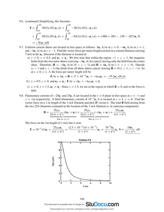
![9.9. A current of −100az A/m flows on the conducting cylinder ρ = 5 mm and +500az A/m is present
on the conducting cylinder ρ = 1 mm. Find the magnitude of the total force acting to split the outer
cylinder apart along its length: The differential force acting on the outer cylinder arising from the field
of the inner cylinder is dF = Kouter × B, where B is the field from the inner cylinder, evaluated at the
outer cylinder location:
B =
2π(1)(500)µ0
2π(5)
aφ = 100µ0 aφ T
Thus dF = −100az × 100µ0aφ = 104µ0aρ N/m2. We wish to find the force acting to split the outer
cylinder, which means we need to evaluate the net force in one cartesian direction on one half of the
cylinder. We choose the “upper” half (0 < φ < π), and integrate the y component of dF over this
range, and over a unit length in the z direction:
Fy =
1
0
π
0
104
µ0aρ · ay(5 × 10⁻³
) dφ dz =
π
0
50µ0 sin φ dφ = 100µ0 = 4π × 10−5
N/m
Note that we did not include the “self force” arising from the outer cylinder’s B field on itself. Since the
outer cylinder is a two-dimensional current sheet, its field exists only just outside the cylinder, and so no
force exists. If this cylinder possessed a finite thickness, then we would need to include its self-force,
since there would be an interior field and a volume current density that would spatially overlap.
9.10. Two infinitely-long parallel filaments each carry 50 A in the az direction. If the filaments lie in the
plane y = 0 at x = 0 and x = 5mm (note bad wording in problem statement in book), find the vector
force per meter length on the filament passing through the origin: The force will be
F =
1
0
IdL × B
where IdL is that of the filament at the origin, and B is that arising from the filament at x = 5mm
evaluated at the location of the other filament (along the z axis). We obtain
F =
1
0
50 dzaz ×
−50µ0ay
2π(5 × 10⁻³)
= 0.10 ax N/m
9.11. a) Use Eq. (14), Sec. 9.3, to show that the force of attraction per unit length between two filamentary
conductors in free space with currents I1az at x = 0, y = d/2, and I2az at x = 0, y = −d/2, is
µ0I1I2/(2πd): The force on I2 is given by
F2 = µ0
I1I2
4π
aR12 × dL1
R2
12
× dL2
Let z1 indicate the z coordinate along I1, and z2 indicate the z coordinate along I2. We then have
R12 = (z2 − z1)2 + d2 and
aR12 =
(z2 − z1)az − day
(z2 − z1)2 + d2
Also, dL1 = dz1az and dL2 = dz2az The “inside” integral becomes:
aR12 × dL1
R2
12
=
[(z2 − z1)az − day] × dz1az
[(z2 − z1)2 + d2]1.5
=
∞
−∞
−d dz1 ax
[(z2 − z1)2 + d2]1.5
147
Descargado por mauricio cartagena (rene_cartagena@yahoo.com)
lOMoARcPSD|5423334](https://image.slidesharecdn.com/solucionario-teoria-electromagnetica-hayt-2001-201211183707/85/Solucionario-teoria-electromagnetica-hayt-2001-149-320.jpg)
![9.11a. (continued) The force expression now becomes
F2 = µ0
I1I2
4π
∞
−∞
−d dz1 ax
[(z2 − z1)2 + d2]1.5
× dz2az = µ0
I1I2
4π
1
0
∞
−∞
d dz1 dz2 ay
[(z2 − z1)2 + d2]1.5
Note that the “outside” integral is taken over a unit length of current I2. Evaluating, obtain,
F2 = µ0
I1I2d ay
4πd2
(2)
1
0
dz2 =
µ0I1I2
2πd
ay N/m
as expected.
b) Show how a simpler method can be used to check your result: We use dF2 = I2dL2 × B12, where
the field from current 1 at the location of current 2 is
B12 =
µ0I1
2πd
ax T
so over a unit length of I2, we obtain
F2 = I2az ×
µ0I1
2πd
ax = µ0
I1I2
2πd
ay N/m
This second method is really just the first over again, since we recognize the inside integral of the
first method as the Biot-Savart law, used to find the field from current 1 at the current 2 location.
9.12. A conducting current strip carrying K = 12az A/m lies in the x = 0 plane between y = 0.5 and y = 1.5
m. There is also a current filament of I = 5 A in the az direction on the z axis. Find the force exerted
on the:
a) filament by the current strip: We first need to find the field from the current strip at the filament
location. Consider the strip as made up of many adjacent strips of width dy, each carrying
current dIaz = Kdy. The field along the z axis from each differential strip will be dB =
[(Kdyµ0)/(2πy)]ax. The total B field from the strip evaluated along the z axis is therefore
B =
1.5
0.5
12µ0ax
2πy
dy =
6µ0
π
ln
1.5
0.5
ax = 2.64 × 10⁻⁶
ax Wb/m2
Now
F =
1
0
IdL × B =
1
0
5dz az × 2.64 × 10⁻⁶
ax dz = 13.2 ay µN/m
b) strip by the filament: In this case we integrate K ×B over a unit length in z of the strip area, where
B is the field from the filament evaluated on the strip surface:
F =
Area
K × B da =
1
0
1.5
0.5
12az ×
−5µ0ax
2πy
dy =
−30µ0
π
ln(3) ay = −13.2 ay µN/m
148
Descargado por mauricio cartagena (rene_cartagena@yahoo.com)
lOMoARcPSD|5423334](https://image.slidesharecdn.com/solucionario-teoria-electromagnetica-hayt-2001-201211183707/85/Solucionario-teoria-electromagnetica-hayt-2001-150-320.jpg)
![9.14a (continued) The force acting on the segment farther from the y axis will be
F2 = IL × B = 30(3 × 10⁻²
)ay × −350µ0ax = 315µ0 az N
The torque about the origin is now T = R1 × F1 + R2 × F2, where R1 is the vector directed from the
origin to the midpoint of the nearer y-directed segment, and R2 is the vector joining the origin to the
midpoint of the farther y-directed segment. So R1(cm) = ax + 3.5ay and R2(cm) = 3ax + 3.5ay.
Therefore
T0,0,0 = [(ax + 3.5ay) × 10−2
] × −315µ0 az + [(3ax + 3.5ay) × 10−2
] × 315µ0 az
= −6.30µ0ay = −7.92 × 10⁻⁶
ay N−m
b) at the center of the loop: Use T = IS × B where S = (2 × 3) × 10−4 az m2. So
T = 30(6 × 10⁻⁴
az) × (−350µ0 ax) = −7.92 × 10⁻⁶
ay N−m
9.15. A solid conducting filament extends from x = −b to x = b along the line y = 2, z = 0. This filament
carries a current of 3 A in the ax direction. An infinite filament on the z axis carries 5 A in the az
direction. Obtain an expression for the torque exerted on the finite conductor about an origin located
at (0, 2, 0): The differential force on the wire segment arising from the field from the infinite wire is
dF = 3 dx ax ×
5µ0
2πρ
aφ = −
15µ0 cos φ dx
2π
√
x2 + 4
az = −
15µ0x dx
2π(x2 + 4)
az
So now the differential torque about the (0, 2, 0) origin is
dT = RT × dF = x ax × −
15µ0x dx
2π(x2 + 4)
az =
15µ0x2 dx
2π(x2 + 4)
ay
The torque is then
T =
b
−b
15µ0x2 dx
2π(x2 + 4)
ay =
15µ0
2π
ay x − 2 tan−1 x
2
b
−b
= (6 × 10⁻⁶
) b − 2 tan−1 b
2
ay N · m
9.16. Assume that an electron is describing a circular orbit of radius a about a positively-charged nucleus.
a) By selecting an appropriate current and area, show that the equivalent orbital dipole moment is
ea2ω/2, where ω is the electron’s angular velocity: The current magnitude will be I = e
T , where
e is the electron charge and T is the orbital period. The latter is T = 2π/ω, and so I = eω/(2π).
Now the dipole moment magnitude will be m = IA, where A is the loop area. Thus
m =
eω
2π
πa2
=
1
2
ea2
ω //
b) Show that the torque produced by a magnetic field parallel to the plane of the orbit is ea2ωB/2:
With B assumed constant over the loop area, we would have T = m × B. With B parallel to the
loop plane, m and B are orthogonal, and so T = mB. So, using part a, T = ea2ωB/2.
150
Descargado por mauricio cartagena (rene_cartagena@yahoo.com)
lOMoARcPSD|5423334](https://image.slidesharecdn.com/solucionario-teoria-electromagnetica-hayt-2001-201211183707/85/Solucionario-teoria-electromagnetica-hayt-2001-152-320.jpg)
![9.17. (continued) As for the magnetic moment, we have
m = IS =
eω
2π
πa2
=
1
2
ωea2 .
=
1
2
ea2
ω0 −
eB
2me
=
1
2
ω0ea2
−
1
4
e2a2B
me
//
Finally, for a = 6 × 10⁻¹¹ m, B = 0.5 T, we have
ω
ω
=
eB
2me
1
ω
.
=
eB
2me
1
ω0
=
1.60 × 10−19 × 0.5
2 × 9.1 × 10−31 × 3.4 × 1016
= 1.3 × 10⁻⁶
where ω0 = 3.4 × 10¹⁶ sec−1 is found from Problem 16. Finally,
m
m
=
e2a2B
4me
×
2
ωea2
.
=
eB
2meω0
= 1.3 × 10⁻⁶
9.18. Calculate the vector torque on the square loop shown in Fig. 9.16 about an origin at A in the field B,
given:
a) A(0, 0, 0) and B = 100ay mT: The field is uniform and so does not produce any translation of the
loop. Therefore, we may use T = IS × B about any origin, where I = 0.6 A and S = 16az m2.
We find T = 0.6(16)az × 0.100ay = −0.96 ax N−m.
b) A(0, 0, 0) and B = 200ax + 100ay mT: Using the same reasoning as in part a, we find
T = 0.6(16)az × (0.200ax + 0.100ay) = −0.96ax + 1.92ay N−m
c) A(1, 2, 3) and B = 200ax +100ay −300az mT: We observe two things here: 1) The field is again
uniform and so again the torque is independent of the origin chosen, and 2) The field differs from
that of part b only by the addition of a z component. With S in the z direction, this new component
of B will produce no torque, so the answer is the same as part b, or T = −0.96ax + 1.92ay N−m.
d) A(1, 2, 3) and B = 200ax + 100ay − 300az mT for x ≥ 2 and B = 0 elsewhere: Now, force
is acting only on the y-directed segment at x = +2, so we need to be careful, since translation
will occur. So we must use the given origin. The differential torque acting on the differential wire
segment at location (2,y) is dT = R(y) × dF, where
dF = IdL × B = 0.6 dy ay × [0.2ax + 0.1ay − 0.3az] = [−0.18ax − 0.12az] dy
and R(y) = (2, y, 0) − (1, 2, 3) = ax + (y − 2)ay − 3az. We thus find
dT = R(y) × dF = ax + (y − 2)ay − 3az × [−0.18ax − 0.12az] dy
= −0.12(y − 2)ax + 0.66ay + 0.18(y − 2)az dy
The net torque is now
T =
2
−2
−0.12(y − 2)ax + 0.66ay + 0.18(y − 2)az dy = 0.96ax + 2.64ay − 1.44az N−m
152
Descargado por mauricio cartagena (rene_cartagena@yahoo.com)
lOMoARcPSD|5423334](https://image.slidesharecdn.com/solucionario-teoria-electromagnetica-hayt-2001-201211183707/85/Solucionario-teoria-electromagnetica-hayt-2001-154-320.jpg)
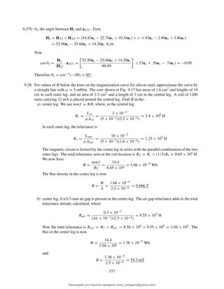
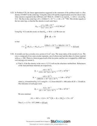
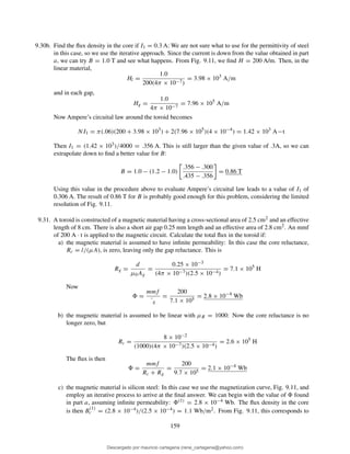
![magnetic field strength H
(1)
c
.
= 270 A/m. We check this by applying Ampere’s circuital law to the
magnetic circuit:
H · dL = H(1)
c Lc + H(1)
g d
where H
(1)
c Lc = (270)(8×10⁻²) = 22, and where H
(1)
g d = (1)¨g = (2.8×10⁻⁴)(7.1×10⁵) =
199. But we require that
H · dL = 200 A · t
whereas the actual result in this first calculation is 199 + 22 = 221, which is too high. So, for a
second trial, we reduce B to B
(2)
c = 1 Wb/m2. This yields H
(2)
c = 200 A/m from Fig. 9.11, and
thus (2) = 2.5 × 10⁻⁴ Wb. Now
H · dL = H(2)
c Lc + (2)
Rg = 200(8 × 10⁻²
) + (2.5 × 10⁻⁴
)(7.1 × 10⁵
) = 194
This is less than 200, meaning that the actual flux is slightly higher than 2.5 × 10⁻⁴ Wb.
I will leave the answer at that, considering the lack of fine resolution in Fig. 9.11.
9.32. Determine the total energy stored in a spherical region 1cm in radius, centered at the origin in free
space, in the uniform field:
a) H1 = −600ay A/m: First we find the energy density:
wm1 =
1
2
B1 · H1 =
1
2
µ0H2
1 =
1
2
(4π × 10−7
)(600)2
= 0.226 J/m3
The energy within the sphere is then
Wm1 = wm1
4
3
πa3
= 0.226
4
3
π × 10−6
= 0.947 µJ
b) H2 = 600ax + 1200ay A/m: In this case the energy density is
wm2 =
1
2
µ0 (600)2
+ (1200)2
=
5
2
µ0(600)2
or five times the energy density that was found in part a. Therefore, the stored energy in this field
is five times the amount in part a, or Wm2 = 4.74 µJ.
c) H3 = −600ax + 1200ay. This field differs from H2 only by the negative x component, which is a
non-issue since the component is squared when finding the energy density. Therefore, the stored
energy will be the same as that in part b, or Wm3 = 4.74 µJ.
d) H4 = H2 + H3, or 2400ay A/m: The energy density is now wm4 = (1/2)µ0(2400)2 =
(1/2)µ0(16)(600)2 J/m3, which is sixteen times the energy density in part a. The stored en-
ergy is therefore sixteen times that result, or Wm4 = 16(0.947) = 15.2 µJ.
e) 1000ax A/m+0.001ax T: The energy density is wm5 = (1/2)µ0[1000+.001/µ0]2 = 2.03 J/m3.
Then Wm5 = 2.03[(4/3)π × 10−6] = 8.49 µJ.
160
Descargado por mauricio cartagena (rene_cartagena@yahoo.com)
lOMoARcPSD|5423334](https://image.slidesharecdn.com/solucionario-teoria-electromagnetica-hayt-2001-201211183707/85/Solucionario-teoria-electromagnetica-hayt-2001-162-320.jpg)
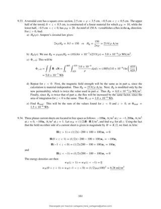
![9.35. The cones θ = 21◦ and θ = 159◦ are conducting surfaces and carry total currents of 40 A, as shown in
Fig. 9.18. The currents return on a spherical conducting surface of 0.25 m radius.
a) Find H in the region 0 < r < 0.25, 21◦ < θ < 159◦, 0 < φ < 2π: We can apply Ampere’s
circuital law and take advantage of symmetry. We expect to see H in the aφ direction and it would
be constant at a given distance from the z axis. We thus perform the line integral of H over a circle,
centered on the z axis, and parallel to the xy plane:
H · dL =
2π
0
Hφaφ · r sin θaφ dφ = Iencl. = 40 A
Assuming that Hφ is constant over the integration path, we take it outside the integral and solve:
Hφ =
40
2πr sin θ
⇒ H =
20
πr sin θ
aφ A/m
b) How much energy is stored in this region? This will be
WH =
v
1
2
µ0H2
φ =
2π
0
159◦
21◦
.25
0
200µ0
π2r2 sin2 θ
r2
sin θ dr dθ dφ =
100µ0
π
159◦
21◦
dθ
sin θ
=
100µ0
π
ln
tan(159/2)
tan(21/2)
= 1.35 × 10⁻⁴
J
9.36. A filament carrying current I in the az direction lies on the z axis, and cylindrical current sheets of 5az
A/m and −2az A/m are located at ρ = 3 and ρ = 10, respectively.
a) Find I if H = 0 for ρ > 10. Ampere’s circuital law says, for ρ > 10:
2πρH = 2π(3)(5) − 2π(10)(2) + I = 0
from which I = 2π(10)(3) − 2π(3)(5) = 10π A.
b) Using this value of I, calculate H for all ρ, 3 < ρ < 10: Again, using Ampere’s circuital law, we
find
H(3 < ρ < 10) =
1
2πρ
[10π + 2π(3)(5)] aφ =
20
ρ
aφ A/m
c) Calculate and plot WH versus ρ0, where WH is the total energy stored within the volume 0 < z < 1,
0 < φ < 2π, 3 < ρ < ρ0: First the energy density will be wH = (1/2)µ0H2 = 200µ0/ρ2 J/m3.
Then the energy is
WH =
1
0
2π
0
ρ0
3
200µ0
ρ2
ρ dρ dφ dz = 400πµ0 ln
ρ0
3
= (1.58 × 10⁻³
) ln
ρ0
3
J
162
Descargado por mauricio cartagena (rene_cartagena@yahoo.com)
lOMoARcPSD|5423334](https://image.slidesharecdn.com/solucionario-teoria-electromagnetica-hayt-2001-201211183707/85/Solucionario-teoria-electromagnetica-hayt-2001-164-320.jpg)
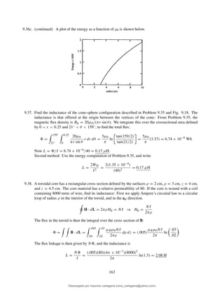
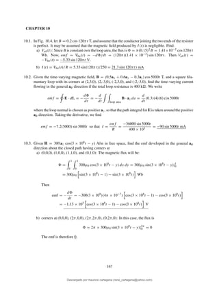
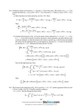
![Then
emf = −
d
dt
=
0.16
3
(3)(5t +2t3
)2
(5+6t2
) = −(0.16)[5(.4)+2(.4)3
]2
[5+6(.4)2
] = −4.32 V
b) x = 0.6 m: Have 0.6 = 5t + 2t3, from which we find t = 0.1193. Thus
emf = −(0.16)[5(.1193) + 2(.1193)3
]2
[5 + 6(.1193)2
] = −.293 V
10.6. A perfectly conducting filament containing a small 500- resistor is formed into a square, as illustrated
in Fig. 10.6. Find I(t) if
a) B = 0.3 cos(120πt −30◦) az T: First the flux through the loop is evaluated, where the unit normal
to the loop is az. We find
=
loop
B · dS = (0.3)(0.5)2
cos(120πt − 30◦
) Wb
Then the current will be
I(t) =
emf
R
= −
1
R
d
dt
=
(120π)(0.3)(0.25)
500
sin(120πt − 30◦
) = 57 sin(120πt − 30◦
) mA
b) B = 0.4 cos[π(ct − y)] az µT where c = 3 × 10⁸ m/s: Since the field varies with y, the flux is
now
=
loop
B · dS = (0.5)(0.4)
.5
0
cos(πy − πct) dy =
0.2
π
[sin(πct − π/2) − sin(πct)] µWb
The current is then
I(t) =
emf
R
= −
1
R
d
dt
=
−0.2c
500
[cos(πct − π/2) − cos(πct)] µA
=
−0.2(3 × 10⁸)
500
[sin(πct) − cos(πct)] µA = 120 [cos(πct) − sin(πct)] mA
10.7. The rails in Fig. 10.7 each have a resistance of 2.2 /m. The bar moves to the right at a constant speed
of 9 m/s in a uniform magnetic field of 0.8 T. Find I(t), 0 < t < 1 s, if the bar is at x = 2 m at t = 0
and
a) a 0.3 resistor is present across the left end with the right end open-circuited: The flux in the
left-hand closed loop is
l = B × area = (0.8)(0.2)(2 + 9t)
Then, emfl = −d l/dt = −(0.16)(9) = −1.44 V. With the bar in motion, the loop resistance is
increasing with time, and is given by Rl(t) = 0.3 + 2[2.2(2 + 9t)]. The current is now
Il(t) =
emfl
Rl(t)
=
−1.44
9.1 + 39.6t
A
Note that the sign of the current indicates that it is flowing in the direction opposite that shown in
the figure.
169
Descargado por mauricio cartagena (rene_cartagena@yahoo.com)
lOMoARcPSD|5423334](https://image.slidesharecdn.com/solucionario-teoria-electromagnetica-hayt-2001-201211183707/85/Solucionario-teoria-electromagnetica-hayt-2001-171-320.jpg)
![b) Repeat part a, but with a resistor of 0.3 across each end: In this case, there will be a contribution
to the current from the right loop, which is now closed. The flux in the right loop, whose area
decreases with time, is
r = (0.8)(0.2)[(16 − 2) − 9t]
and emfr = −d r/dt = (0.16)(9) = 1.44 V. The resistance of the right loop is Rr(t) =
0.3 + 2[2.2(14 − 9t)], and so the contribution to the current from the right loop will be
Ir(t) =
−1.44
61.9 − 39.6t
A
The minus sign has been inserted because again the current must flow in the opposite direction
as that indicated in the figure, with the flux decreasing with time. The total current is found by
adding the part a result, or
IT (t) = −1.44
1
61.9 − 39.6t
+
1
9.1 + 39.6t
A
10.8. Fig. 10.1 is modified to show that the rail separation is larger when y is larger. Specifically, let the
separation d = 0.2 + 0.02y. Given a uniform velocity vy = 8 m/s and a uniform magnetic flux density
Bz = 1.1 T, find V12 as a function of time if the bar is located at y = 0 at t = 0: The flux through the
loop as a function of y can be written as
= B · dS =
y
0
.2+.02y′
0
1.1 dx dy′
=
y
0
1.1(.2 + .02y′
) dy′
= 0.22y(1 + .05y)
Now, with y = vt = 8t, the above becomes = 1.76t(1 + .40t). Finally,
V12 = −
d
dt
= −1.76(1 + .80t) V
10.9. A square filamentary loop of wire is 25 cm on a side and has a resistance of 125 per meter length. The
loop lies in the z = 0 plane with its corners at (0, 0, 0), (0.25, 0, 0), (0.25, 0.25, 0), and (0, 0.25, 0) at
t = 0. The loop is moving with velocity vy = 50 m/s in the field Bz = 8 cos(1.5 × 10⁸t − 0.5x) µT.
Develop a function of time which expresses the ohmic power being delivered to the loop: First, since
the field does not vary with y, the loop motion in the y direction does not produce any time-varying
flux, and so this motion is immaterial. We can evaluate the flux at the original loop position to obtain:
(t) =
.25
0
.25
0
8 × 10⁻⁶
cos(1.5 × 10⁸
t − 0.5x) dx dy
= −(4 × 10⁻⁶
) sin(1.5 × 10⁸
t − 0.13x) − sin(1.5 × 10⁸
t) Wb
Now, emf = V (t) = −d /dt = 6.0 × 10² cos(1.5 × 10⁸t − 0.13x) − cos(1.5 × 10⁸t) , The total
loop resistance is R = 125(0.25 + 0.25 + 0.25 + 0.25) = 125 . Then the ohmic power is
P (t) =
V 2(t)
R
= 2.9 × 10³
cos(1.5 × 10⁸
t − 0.13x) − cos(1.5 × 10⁸
t) Watts
170
Descargado por mauricio cartagena (rene_cartagena@yahoo.com)
lOMoARcPSD|5423334](https://image.slidesharecdn.com/solucionario-teoria-electromagnetica-hayt-2001-201211183707/85/Solucionario-teoria-electromagnetica-hayt-2001-172-320.jpg)
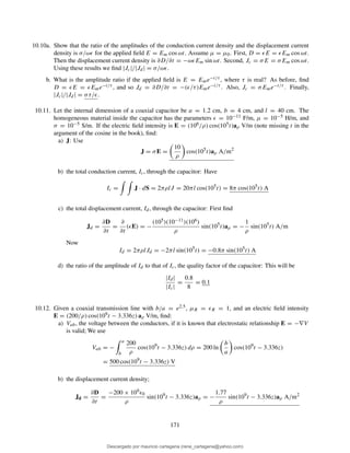
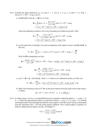
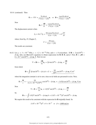
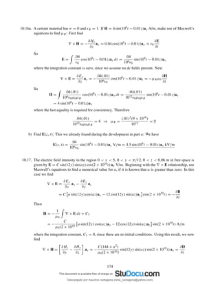
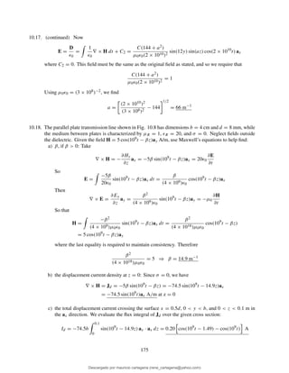
![10.19. In the first section of this chapter, Faraday’s law was used to show that the field E = −1
2 kB0ρekt aφ
results from the changing magnetic field B = B0ekt az (note that the factor of ρ appearing in E was
omitted from the original problem statement).
a) Show that these fields do not satisfy Maxwell’s other curl equation: Note that B as stated is constant
with position, and so will have zero curl. The electric field, however, varies with time, and so
∇ × H = ∂D
∂t would have a zero left-hand side and a non-zero right-hand side. The equation is
thus not valid with these fields.
b) If we let B0 = 1 T and k = 106 s−1, we are establishing a fairly large magnetic flux density in 1
µs. Use the ∇ × H equation to show that the rate at which Bz should (but does not) change with
ρ is only about 5 × 10⁻⁶ T/m in free space at t = 0: Assuming that B varies with ρ, we write
∇ × H = −
∂Hz
∂ρ
aφ = −
1
µ0
dB0
dρ
ekt
= ǫ0
∂E
∂t
= −
1
2
ǫ0k2
B0ρekt
Thus
dB0
dρ
=
1
2
µ0ǫ0k2
ρB0 =
1012(1)ρ
2(3 × 10⁸)2
= 5.6 × 10⁻⁶
ρ
which is near the stated value if ρ is on the order of 1m.
10.20. Point C(−0.1, −0.2, 0.3) lies on the surface of a perfect conductor. The electric field intensity at C is
(500ax − 300ay + 600az) cos 107t V/m, and the medium surrounding the conductor is characterized
by µR = 5, ǫR = 10, and σ = 0.
a) Find a unit vector normal to the conductor surface at C, if the origin lies within the conductor:
At t = 0, the field must be directed out of the surface, and will be normal to it, since we have a
perfect conductor. Therefore
n =
+E(t = 0)
|E(t = 0)|
=
5ax − 3ay + 6az
√
25 + 9 + 36
= 0.60ax − 0.36ay + 0.72az
b) Find the surface charge density at C: Use
ρs = D · n|surf ace = 10ǫ0 500ax − 300ay + 600az cos(107
t) · .60ax − .36ay + .72az
= 10ǫ0 [300 + 108 + 432] cos(107
t) = 7.4 × 10⁻⁸
cos(107
t) C/m2
= 74 cos(107
t) nC/m2
10.21. The surfaces ρ = 3 and 10 mm, and z = 0 and 25 cm are perfect conductors. The region en-
closed by these surfaces has µ = 2.5 × 10⁻⁶ H/m, ǫ = 4 × 10⁻¹¹ F/m, and σ = 0. Let H =
(2/ρ) cos(10πz) cos(ωt) aφ A/m. Make use of Maxwell’s equations to find
a) ω: We start with
∇ × H = −
∂Hφ
∂z
aρ =
20π
ρ
sin(10πz) cos(ωt) aρ = ǫ
∂E
∂t
We then find
E =
20π
ρǫ
sin(10πz) cos(ωt) dt aρ =
20π
ωρǫ
sin(10πz) sin(ωt) aρ
176
Descargado por mauricio cartagena (rene_cartagena@yahoo.com)
lOMoARcPSD|5423334](https://image.slidesharecdn.com/solucionario-teoria-electromagnetica-hayt-2001-201211183707/85/Solucionario-teoria-electromagnetica-hayt-2001-178-320.jpg)
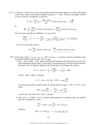
![10.23. (continued)
These, along with the permittivities and conductivities, are substituted to obtain
(4 × 10⁻³
)(10) cos(109
t) − 10−3
[A cos(109
t) + B sin(109
t)]
=
∂
∂t
10−11
[A cos(109
t) + B sin(109
t)] − (2 × 10⁻¹¹
)(10) cos(109
t)
= −(10−2
A sin(109
t) + 10−2
B cos(109
t) + (2 × 10⁻¹
) sin(109
t)
We now equate coefficients of the sin and cos terms to obtain two equations:
4 × 10⁻²
− 10−3
A = 10−2
B
−10−3
B = −10−2
A + 2 × 10⁻¹
These are solved together to find A = 20.2 and B = 2.0. Thus
EN2 = 20.2 cos(109
t) + 2.0 sin(109
t) az = 20.3 cos(109
t + 5.6◦
)az V/m
Then
DN2 = ǫ2EN2 = 203 cos(109
t + 5.6◦
)az pC/m2
and
JN2 = σ2EN2 = 20.3 cos(109
t + 5.6◦
)az mA/m2
10.24. Given the fields V = 80z cos x cos 3 × 10⁸t. kV and A = 26.7z sin x sin 3 × 10⁸t ax mWb/m in free
space, find E and H: First, find E through
E = −∇V −
∂A
∂t
where
−∇V = 80 cos(3 × 10⁸
t)[z sin xax − cos xaz] kV/m
and
−∂A/∂t = −(3 × 10⁸
)(26.7)z sin x cos(3 × 10⁸
t)ax mV/m
Finally,
E = − 7.9 × 10⁶
z sin x ax + 8.0 × 10⁴
cos x az cos(3 × 10⁸
t) V/m
Now
B = ∇ × A =
∂Ax
∂z
ay = 26.7 sin x sin(3 × 10⁸
t)ay mWb/m2
Then
H =
B
µ0
= 2.12 × 10⁴
sin x sin(3 × 10⁸
t) ay A/m
179
Descargado por mauricio cartagena (rene_cartagena@yahoo.com)
lOMoARcPSD|5423334](https://image.slidesharecdn.com/solucionario-teoria-electromagnetica-hayt-2001-201211183707/85/Solucionario-teoria-electromagnetica-hayt-2001-181-320.jpg)
![10.25. In a region where µR = ǫR = 1 and σ = 0, the retarded potentials are given by V = x(z − ct) V and
A = x[(z/c) − t]az Wb/m, where c = 1/
√
µ0ǫ0.
a) Show that ∇ · A = −µǫ(∂V/∂t):
First,
∇ · A =
∂Az
∂z
=
x
c
= x
√
µ0ǫ0
Second,
∂V
∂t
= −cx = −
x
√
µ0ǫ0
so we observe that ∇ · A = −µ0ǫ0(∂V/∂t) in free space, implying that the given statement would
hold true in general media.
b) Find B, H, E, and D:
Use
B = ∇ × A = −
∂Ax
∂x
ay = t −
z
c
ay T
Then
H =
B
µ0
=
1
µ0
t −
z
c
ay A/m
Now,
E = −∇V −
∂A
∂t
= −(z − ct)ax − xaz + xaz = (ct − z)ax V/m
Then
D = ǫ0E = ǫ0(ct − z)ax C/m2
c) Show that these results satisfy Maxwell’s equations if J and ρv are zero:
i. ∇ · D = ∇ · ǫ0(ct − z)ax = 0
ii. ∇ · B = ∇ · (t − z/c)ay = 0
iii.
∇ × H = −
∂Hy
∂z
ax =
1
µ0c
ax =
ǫ0
µ0
ax
which we require to equal ∂D/∂t:
∂D
∂t
= ǫ0cax =
ǫ0
µ0
ax
iv.
∇ × E =
∂Ex
∂z
ay = −ay
which we require to equal −∂B/∂t:
∂B
∂t
= ay
So all four Maxwell equations are satisfied.
180
Descargado por mauricio cartagena (rene_cartagena@yahoo.com)
lOMoARcPSD|5423334](https://image.slidesharecdn.com/solucionario-teoria-electromagnetica-hayt-2001-201211183707/85/Solucionario-teoria-electromagnetica-hayt-2001-182-320.jpg)
![CHAPTER 11
11.1. Show that Exs = Aejk0z+φ is a solution to the vector Helmholtz equation, Sec. 11.1, Eq. (16), for
k0 = ω
√
µ0ǫ0 and any φ and A: We take
d2
dz2
Aejk0z+φ
= (jk0)2
Aejk0z+φ
= −k2
0Exs
11.2. Let E(z, t) = 200 sin 0.2z cos 108tax + 500 cos(0.2z + 50◦) sin 108tay V/m. Find:
a) E at P (0, 2, 0.6) at t = 25 ns: Obtain
EP (t = 25) = 200 sin [(0.2)(0.6)] cos(2.5)ax + 500 cos [(0.2)(0.6) + 50(2π)/360] sin(2.5)ay
= −19.2ax + 164ay V/m
b) |E| at P at t = 20 ns:
EP (t = 20) = 200 sin [(0.2)(0.6)] cos(2.0)ax + 500 cos [(0.2)(0.6) + 50(2π)/360] sin(2.0)ay
= −9.96ax + 248ay V/m
Thus |EP | = (9.96)2 + (248)2 = 249 V/m.
c) Es at P: Es = 200 sin 0.2zax − j500 cos(0.2z + 50◦)ay. Thus
EsP = 200 sin [(0.2)(0.6)] ax − j500 cos [(0.2)(0.6) + 2π(50)/360] ay
= 23.9ax − j273ay V/m
11.3. An H field in free space is given as H(x, t) = 10 cos(108t − βx)ay A/m. Find
a) β: Since we have a uniform plane wave, β = ω/c, where we identify ω = 108 sec−1. Thus
β = 108/(3 × 108) = 0.33 rad/m.
b) λ: We know λ = 2π/β = 18.9 m.
c) E(x, t) at P (0.1, 0.2, 0.3) at t = 1 ns: Use E(x, t) = −η0H(x, t) = −(377)(10) cos(108t −
βx) = −3.77 × 10³ cos(108t − βx). The vector direction of E will be −az, since we require that
S = E × H, where S is x-directed. At the given point, the relevant coordinate is x = 0.1. Using
this, along with t = 10−9 sec, we finally obtain
E(x, t) = −3.77 × 10³
cos[(108
)(10−9
) − (0.33)(0.1)]az = −3.77 × 10³
cos(6.7 × 10⁻²
)az
= −3.76 × 10³
az V/m
11.4. In phasor form, the electric field intensity of a uniform plane wave in free space is expressed as
Es = (40 − j30)e−j20zax V/m. Find:
a) ω: From the given expression, we identify β = 20 rad/m. Then ω = cβ = (3 × 10⁸)(20) =
6.0 × 10⁹ rad/s.
b) β = 20 rad/m from part a.
182
Descargado por mauricio cartagena (rene_cartagena@yahoo.com)
lOMoARcPSD|5423334](https://image.slidesharecdn.com/solucionario-teoria-electromagnetica-hayt-2001-201211183707/85/Solucionario-teoria-electromagnetica-hayt-2001-184-320.jpg)
![11.4. (continued)
c) f = ω/2π = 956 MHz.
d) λ = 2π/β = 2π/20 = 0.314 m.
e) Hs: In free space, we find Hs by dividing Es by η0, and assigning vector components such that
Es × Hs gives the required direction of wave travel: We find
Hs =
40 − j30
377
e−j20z
ay = (0.11 − j0.08)e−j20z
ay A/m
f) H(z, t) at P (6, −1, 0.07), t = 71 ps:
H(z, t) = Re Hsejωt
= 0.11 cos(6.0 × 10⁹
t − 20z) + 0.08 sin(6.0 × 10⁹
t − 20z) ay
Then
H(.07, t = 71ps) = 0.11 cos (6.0 × 10⁹
)(7.1 × 10⁻¹¹
) − 20(.07)
+ .08 sin (6.0 × 10⁹
)(7.1 × 10⁻¹¹
) − 20(.07) ay
= [0.11(0.562) − 0.08(0.827)]ay = −6.2 × 10⁻³
ay A/m
11.5. A 150-MHz uniform plane wave in free space is described by Hs = (4 + j10)(2ax + jay)e−jβz A/m.
a) Find numerical values for ω, λ, and β: First, ω = 2π × 150 × 106 = 3π × 108 sec−1. Second,
for a uniform plane wave in free space, λ = 2πc/ω = c/f = (3 × 10⁸)/(1.5 × 108) = 2 m.
Third, β = 2π/λ = π rad/m.
b) Find H(z, t) at t = 1.5 ns, z = 20 cm: Use
H(z, t) = Re{Hsejωt
} = Re{(4 + j10)(2ax + jay)(cos(ωt − βz) + j sin(ωt − βz)}
= [8 cos(ωt − βz) − 20 sin(ωt − βz)] ax − [10 cos(ωt − βz) + 4 sin(ωt − βz)] ay
. Now at the given position and time, ωt − βz = (3π × 108)(1.5 × 10⁻⁹) − π(0.20) = π/4. And
cos(π/4) = sin(π/4) = 1/
√
2. So finally,
H(z = 20cm, t = 1.5ns) = −
1
√
2
12ax + 14ay = −8.5ax − 9.9ay A/m
c) What is |E|max? Have |E|max = η0|H|max, where
|H|max = Hs · H∗
s = [4(4 + j10)(4 − j10) + (j)(−j)(4 + j10)(4 − j10)]1/2
= 24.1 A/m
Then |E|max = 377(24.1) = 9.08 kV/m.
183
Descargado por mauricio cartagena (rene_cartagena@yahoo.com)
lOMoARcPSD|5423334](https://image.slidesharecdn.com/solucionario-teoria-electromagnetica-hayt-2001-201211183707/85/Solucionario-teoria-electromagnetica-hayt-2001-185-320.jpg)
![11.8. Let the fields, E(z, t) = 1800 cos(107πt − βz)ax V/m and H(z, t) = 3.8 cos(107πt − βz)ay A/m,
represent a uniform plane wave propagating at a velocity of 1.4 × 10⁸ m/s in a perfect dielectric. Find:
a) β = ω/v = (107π)/(1.4 × 108) = 0.224 m−1.
b) λ = 2π/β = 2π/.224 = 28.0 m.
c) η = |E|/|H| = 1800/3.8 = 474 .
d) µR: Have two equations in the two unknowns, µR and ǫR: η = η0
√
µR/ǫR and β = ω
√
µRǫR/c.
Eliminate ǫR to find
µR =
βcη
ωη0
2
=
(.224)(3 × 10⁸)(474)
(107π)(377)
2
= 2.69
e) ǫR = µR(η0/η)2 = (2.69)(377/474)2 = 1.70.
11.9. A certain lossless material has µR = 4 and ǫR = 9. A 10-MHz uniform plane wave is propagating in
the ay direction with Ex0 = 400 V/m and Ey0 = Ez0 = 0 at P (0.6, 0.6, 0.6) at t = 60 ns.
a) Find β, λ, vp, and η: For a uniform plane wave,
β = ω
√
µǫ =
ω
c
√
µRǫR =
2π × 107
3 × 10⁸
(4)(9) = 0.4π rad/m
Then λ = (2π)/β = (2π)/(0.4π) = 5 m. Next,
vp =
ω
β
=
2π × 107
4π × 10−1
= 5 × 10⁷
m/s
Finally,
η =
µ
ǫ
= η0
µR
ǫR
= 377
4
9
= 251
b) Find E(t) (at P ): We are given the amplitude at t = 60 ns and at y = 0.6 m. Let the maximum
amplitude be Emax, so that in general, Ex = Emax cos(ωt − βy). At the given position and time,
Ex = 400 = Emax cos[(2π × 107
)(60 × 10−9
) − (4π × 10−1
)(0.6)] = Emax cos(0.96π)
= −0.99Emax
So Emax = (400)/(−0.99) = −403 V/m. Thus at P, E(t) = −403 cos(2π × 107t) V/m.
c) Find H(t): First, we note that if E at a given instant points in the negative x direction, while the
wave propagates in the forward y direction, then H at that same position and time must point in
the positive z direction. Since we have a lossless homogeneous medium, η is real, and we are
allowed to write H(t) = E(t)/η, where η is treated as negative and real. Thus
H(t) = Hz(t) =
Ex(t)
η
=
−403
−251
cos(2π × 10−7
t) = 1.61 cos(2π × 10−7
t) A/m
185
Descargado por mauricio cartagena (rene_cartagena@yahoo.com)
lOMoARcPSD|5423334](https://image.slidesharecdn.com/solucionario-teoria-electromagnetica-hayt-2001-201211183707/85/Solucionario-teoria-electromagnetica-hayt-2001-187-320.jpg)
![11.12. The plane wave Es = 300e−jkxay V/m is propagating in a material for which µ = 2.25 µH/m, ǫ′ = 9
pF/m, and ǫ′′ = 7.8 pF/m. If ω = 64 Mrad/s, find:
a) α: We use the general formula, Eq. (35):
α = ω
µǫ′
2
1 +
ǫ′′
ǫ′
2
− 1
1/2
= (64 × 106
)
(2.25 × 10⁻⁶)(9 × 10⁻¹²)
2
1 + (.867)2 − 1
1/2
= 0.116 Np/m
b) β: Using (36), we write
β = ω
µǫ′
2
1 +
ǫ′′
ǫ′
2
+ 1
1/2
= .311 rad/m
c) vp = ω/β = (64 × 106)/(.311) = 2.06 × 10⁸ m/s.
d) λ = 2π/β = 2π/(.311) = 20.2 m.
e) η: Using (39):
η =
µ
ǫ′
1
1 − j(ǫ′′/ǫ′)
=
2.25 × 10⁻⁶
9 × 10⁻¹²
1
√
1 − j(.867)
= 407 + j152 = 434.5ej.36
f) Hs: With Es in the positive y direction (at a given time) and propagating in the positive x direction,
we would have a positive z component of Hs, at the same time. We write (with jk = α + jβ):
Hs =
Es
η
az =
300
434.5ej.36
e−jkx
az = 0.69e−αx
e−jβx
e−j.36
az
= 0.69e−.116x
e−j.311x
e−j.36
az A/m
g) E(3, 2, 4, 10ns): The real instantaneous form of E will be
E(x, y, z, t) = Re Esejωt
= 300e−αx
cos(ωt − βx)ay
Therefore
E(3, 2, 4, 10ns) = 300e−.116(3)
cos[(64 × 106
)(10−8
) − .311(3)]ay = 203 V/m
11.13. Let jk = 0.2 + j1.5 m−1 and η = 450 + j60 for a uniform plane wave propagating in the az
direction. If ω = 300 Mrad/s, find µ, ǫ′, and ǫ′′: We begin with
η =
µ
ǫ′
1
1 − j(ǫ′′/ǫ′)
= 450 + j60
and
jk = jω µǫ′ 1 − j(ǫ′′/ǫ′) = 0.2 + j1.5
187
Descargado por mauricio cartagena (rene_cartagena@yahoo.com)
lOMoARcPSD|5423334](https://image.slidesharecdn.com/solucionario-teoria-electromagnetica-hayt-2001-201211183707/85/Solucionario-teoria-electromagnetica-hayt-2001-189-320.jpg)
![11.13. (continued) Then
ηη∗
=
µ
ǫ′
1
1 + (ǫ′′/ǫ′)2
= (450 + j60)(450 − j60) = 2.06 × 10⁵
(1)
and
(jk)(jk)∗
= ω2
µǫ′
1 + (ǫ′′/ǫ′)2 = (0.2 + j1.5)(0.2 − j1.5) = 2.29 (2)
Taking the ratio of (2) to (1),
(jk)(jk)∗
ηη∗
= ω2
(ǫ′
)2
1 + (ǫ′′
/ǫ′
)2
=
2.29
2.06 × 105
= 1.11 × 10⁻⁵
Then with ω = 3 × 10⁸,
(ǫ′
)2
=
1.11 × 10⁻⁵
(3 × 10⁸)2 1 + (ǫ′′/ǫ′)2
=
1.23 × 10⁻²²
1 + (ǫ′′/ǫ′)2
(3)
Now, we use Eqs. (35) and (36). Squaring these and taking their ratio gives
α2
β2
=
1 + (ǫ′′/ǫ′)2
1 + (ǫ′′/ǫ′)2
=
(0.2)2
(1.5)2
We solve this to find ǫ′′/ǫ′ = 0.271. Substituting this result into (3) gives ǫ′ = 1.07 × 10⁻¹¹ F/m.
Since ǫ′′/ǫ′ = 0.271, we then find ǫ′′ = 2.90 × 10⁻¹² F/m. Finally, using these results in either (1) or
(2) we find µ = 2.28 × 10⁻⁶ H/m. Summary: µ = 2.28 × 10⁻⁶ H/m,
ǫ′ = 1.07 × 10⁻¹¹ F/m, and ǫ′′ = 2.90 × 10⁻¹² F/m.
11.14. A certain nonmagnetic material has the material constants ǫ′
R = 2 and ǫ′′/ǫ′ = 4 × 10⁻⁴ at ω = 1.5
Grad/s. Find the distance a uniform plane wave can propagate through the material before:
a) it is attenuated by 1 Np: First, ǫ′′ = (4 × 10⁴)(2)(8.854 × 10⁻¹²) = 7.1 × 10⁻¹⁵ F/m. Then,
since ǫ′′/ǫ′ << 1, we use the approximate form for α, given by Eq. (51) (written in terms of ǫ′′):
α
.
=
ωǫ′′
2
µ
ǫ′
=
(1.5 × 10⁹)(7.1 × 10⁻¹⁵)
2
377
√
2
= 1.42 × 10⁻³
Np/m
The required distance is now z1 = (1.42 × 10⁻³)−1 = 706 m
b) the power level is reduced by one-half: The governing relation is e−2αz1/2 = 1/2, or z1/2 =
ln 2/2α = ln 2/2(1.42 × 10−3) = 244 m.
c) the phase shifts 360◦: This distance is defined as one wavelength, where λ = 2π/β
= (2πc)/(ω ǫ′
R) = [2π(3 × 10⁸)]/[(1.5 × 109)
√
2] = 0.89 m.
11.15. A 10 GHz radar signal may be represented as a uniform plane wave in a sufficiently small region.
Calculatethewavelengthincentimetersandtheattenuationinneperspermeterifthewaveispropagating
in a non-magnetic material for which
a) ǫ′
R = 1 and ǫ′′
R = 0: In a non-magnetic material, we would have:
α = ω
µ0ǫ0ǫ′
R
2
1 +
ǫ′′
R
ǫ′
R
2
− 1
1/2
188
Descargado por mauricio cartagena (rene_cartagena@yahoo.com)
lOMoARcPSD|5423334](https://image.slidesharecdn.com/solucionario-teoria-electromagnetica-hayt-2001-201211183707/85/Solucionario-teoria-electromagnetica-hayt-2001-190-320.jpg)
![11.15. (continued) and
β = ω
µ0ǫ0ǫ′
R
2
1 +
ǫ′′
R
ǫ′
R
2
+ 1
1/2
With the given values of ǫ′
R and ǫ′′
R, it is clear that β = ω
√
µ0ǫ0 = ω/c, and so
λ = 2π/β = 2πc/ω = 3 × 10¹⁰/1010 = 3 cm. It is also clear that α = 0.
b) ǫ′
R = 1.04 and ǫ′′
R = 9.00 × 10⁻⁴: In this case ǫ′′
R/ǫ′
R << 1, and so β
.
= ω ǫ′
R/c = 2.13 cm−1.
Thus λ = 2π/β = 2.95 cm. Then
α
.
=
ωǫ′′
2
µ
ǫ′
=
ωǫ′′
R
2
√
µ0ǫ0
ǫ′
R
=
ω
2c
ǫ′′
R
ǫ′
R
=
2π × 1010
2 × 3 × 108
(9.00 × 10⁻⁴)
√
1.04
= 9.24 × 10⁻²
Np/m
c) ǫ′
R = 2.5 and ǫ′′
R = 7.2: Using the above formulas, we obtain
β =
2π × 1010
√
2.5
(3 × 10¹⁰)
√
2
1 +
7.2
2.5
2
+ 1
1/2
= 4.71 cm−1
and so λ = 2π/β = 1.33 cm. Then
α =
2π × 1010
√
2.5
(3 × 10⁸)
√
2
1 +
7.2
2.5
2
− 1
1/2
= 335 Np/m
11.16. The power factor of a capacitor is defined as the cosine of the impedance phase angle, and its Q is
ωCR, where R is the parallel resistance. Assume an idealized parallel plate capacitor having a dielecric
characterized by σ, ǫ′, and µR. Find both the power factor and Q in terms of the loss tangent: First,
the impedance will be:
Z =
R 1
jωC
R + 1
jωC
= R
1 − jRωC
1 + (RωC)2
= R
1 − jQ
1 + Q2
Now R = d/(σA) and C = ǫ′A/d, and so Q = ωǫ′/σ = 1/l.t. Then the power factor is P.F =
cos[tan−1(−Q)] = 1/ 1 + Q2.
189
Descargado por mauricio cartagena (rene_cartagena@yahoo.com)
lOMoARcPSD|5423334](https://image.slidesharecdn.com/solucionario-teoria-electromagnetica-hayt-2001-201211183707/85/Solucionario-teoria-electromagnetica-hayt-2001-191-320.jpg)
![11.22. The inner and outer dimensions of a copper coaxial transmission line are 2 and 7 mm, respectively.
Both conductors have thicknesses much greater than δ. The dielectric is lossless and the operating
frequency is 400 MHz. Calculate the resistance per meter length of the:
a) inner conductor: First
δ =
1
√
πf µσ
=
1
π(4 × 10⁸)(4π × 10−7)(5.8 × 10⁷)
= 3.3 × 10⁻⁶
m = 3.3µm
Now, using (70) with a unit length, we find
Rin =
1
2πaσδ
=
1
2π(2 × 10⁻³)(5.8 × 10⁷)(3.3 × 10⁻⁶)
= 0.42 ohms/m
b) outer conductor: Again, (70) applies but with a different conductor radius. Thus
Rout =
a
b
Rin =
2
7
(0.42) = 0.12 ohms/m
c) transmission line: Since the two resistances found above are in series, the line resistance is their
sum, or R = Rin + Rout = 0.54 ohms/m.
11.23. A hollow tubular conductor is constructed from a type of brass having a conductivity of 1.2 × 10⁷ S/m.
The inner and outer radii are 9 mm and 10 mm respectively. Calculate the resistance per meter length
at a frequency of
a) dc: In this case the current density is uniform over the entire tube cross-section. We write:
R(dc) =
L
σA
=
1
(1.2 × 10⁷)π(.012 − .0092)
= 1.4 × 10⁻³
/m
b) 20 MHz: Now the skin effect will limit the effective cross-section. At 20 MHz, the skin depth is
δ(20MHz) = [πf µ0σ]−1/2
= [π(20 × 106
)(4π × 10−7
)(1.2 × 10⁷
)]−1/2
= 3.25 × 10⁻⁵
m
This is much less than the outer radius of the tube. Therefore we can approximate the resistance
using the formula:
R(20MHz) =
L
σA
=
1
2πbδ
=
1
(1.2 × 10⁷)(2π(.01))(3.25 × 10⁻⁵)
= 4.1 × 10⁻²
/m
c) 2 GHz: Using the same formula as in part b, we find the skin depth at 2 GHz to be δ = 3.25×10⁻⁶
m. The resistance (using the other formula) is R(2GHz) = 4.1 × 10⁻¹ /m.
194
Descargado por mauricio cartagena (rene_cartagena@yahoo.com)
lOMoARcPSD|5423334](https://image.slidesharecdn.com/solucionario-teoria-electromagnetica-hayt-2001-201211183707/85/Solucionario-teoria-electromagnetica-hayt-2001-196-320.jpg)
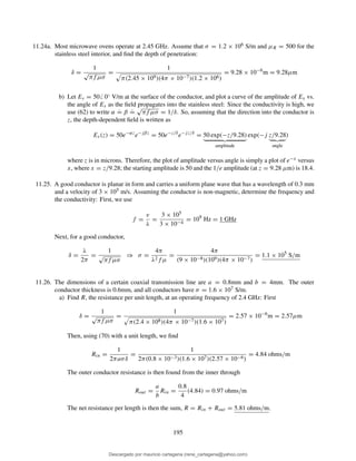
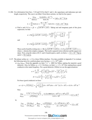
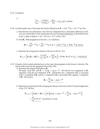
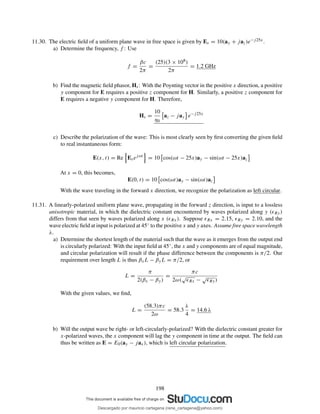
![11.32. Suppose that the length of the medium of Problem 11.31 is made to be twice that as determined in
the problem. Describe the polarization of the output wave in this case: With the length doubled, a
phase shift of π radians develops between the two components. At the input, we can write the field as
Es(0) = E0(ax + ay). After propagating through length L, we would have,
Es(L) = E0[e−jβxL
ax + e−jβyL
ay] = E0e−jβxL
[ax + e−j(βy−βx)L
ay]
where (βy − βx)L = −π (since βx > βy), and so Es(L) = E0e−jβxL[ax − ay]. With the reversal of
the y component, the wave polarization is rotated by 90◦, but is still linear polarization.
11.33. Given a wave for which Es = 15e−jβzax +18e−jβzejφay V/m, propagating in a medium characterized
by complex intrinsic impedance, η.
a) Find Hs: With the wave propagating in the forward z direction, we find:
Hs =
1
η
−18ejφ
ax + 15ay e−jβz
A/m
b) Determine the average power density in W/m2: We find
Pz,avg =
1
2
Re Es × H∗
s =
1
2
Re
(15)2
η∗
+
(18)2
η∗
= 275 Re
1
η∗
W/m2
11.34. Given the general elliptically-polarized wave as per Eq. (73):
Es = [Ex0ax + Ey0ejφ
ay]e−jβz
a) Show, using methods similar to those of Example 11.7, that a linearly polarized wave results when
superimposing the given field and a phase-shifted field of the form:
Es = [Ex0ax + Ey0e−jφ
ay]e−jβz
ejδ
where δ is a constant: Adding the two fields gives
Es,tot = Ex0 1 + ejδ
ax + Ey0 ejφ
+ e−jφ
ejδ
ay e−jβz
=
Ex0ejδ/2
e−jδ/2
+ ejδ/2
2 cos(δ/2)
ax + Ey0ejδ/2
e−jδ/2
ejφ
+ e−jφ
ejδ/2
2 cos(φ−δ/2)
ay
e−jβz
This simplifies to Es,tot = 2 Ex0 cos(δ/2)ax + Ey0 cos(φ − δ/2)ay ejδ/2e−jβz, which is lin-
early polarized.
b) Find δ in terms of φ such that the resultant wave is polarized along x: By inspecting the part a
result, we achieve a zero y component when 2φ − δ = π (or odd multiples of π).
199
Descargado por mauricio cartagena (rene_cartagena@yahoo.com)
lOMoARcPSD|5423334](https://image.slidesharecdn.com/solucionario-teoria-electromagnetica-hayt-2001-201211183707/85/Solucionario-teoria-electromagnetica-hayt-2001-201-320.jpg)
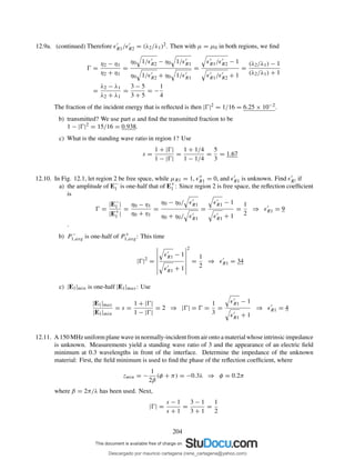
![12.11. (continued) So we now have
Ŵ = 0.5ej0.2π
=
ηu − η0
ηu + η0
We solve for ηu to find
ηu = η0(1.70 + j1.33) = 641 + j501
12.12. A 50MHz uniform plane wave is normally incident from air onto the surface of a calm ocean. For
seawater, σ = 4 S/m, and ǫ′
R = 78.
a) Determine the fractions of the incident power that are reflected and transmitted: First we find the
loss tangent:
σ
ωǫ′
=
4
2π(50 × 106)(78)(8.854 × 10⁻¹²)
= 18.4
This value is sufficiently greater than 1 to enable seawater to be considered a good conductor
at 50MHz. Then, using the approximation (Eq. 65, Chapter 11), the intrinsic impedance is
ηs =
√
πf µ/σ(1 + j), and the reflection coefficient becomes
Ŵ =
√
πf µ/σ (1 + j) − η0
√
πf µ/σ (1 + j) + η0
where
√
πf µ/σ = π(50 × 106)(4π × 10−7)/4 = 7.0. The fraction of the power reflected is
Pr
Pi
= |Ŵ|2
=
[
√
πf µ/σ − η0]2 + πf µ/σ
[
√
πf µ/σ + η0]2 + πf µ/σ
=
[7.0 − 377]2 + 49.0
[7.0 + 377]2 + 49.0
= 0.93
The transmitted fraction is then
Pt
Pi
= 1 − |Ŵ|2
= 1 − 0.93 = 0.07
b) Qualitatively, how will these answers change (if at all) as the frequency is increased? Within
the limits of our good conductor approximation (loss tangent greater than about ten), the reflected
power fraction, using the formula derived in part a, is found to decrease with increasing frequency.
The transmitted power fraction thus increases.
12.13. A right-circularly-polarized plane wave is normally incident from air onto a semi-infinite slab of plex-
iglas (ǫ′
R = 3.45, ǫ′′
R = 0). Calculate the fractions of the incident power that are reflected and trans-
mitted. Also, describe the polarizations of the reflected and transmitted waves. First, the impedance of
the plexiglas will be η = η0/
√
3.45 = 203 . Then
Ŵ =
203 − 377
203 + 377
= −0.30
The reflected power fraction is thus |Ŵ|2 = 0.09. The total electric field in the plane of the interface
must rotate in the same direction as the incident field, in order to continually satisfy the boundary
condition of tangential electric field continuity across the interface. Therefore, the reflected wave will
have to be left circularly polarized in order to make this happen. The transmitted power fraction is now
1 − |Ŵ|2 = 0.91. The transmitted field will be right circularly polarized (as the incident field) for the
same reasons.
205
Descargado por mauricio cartagena (rene_cartagena@yahoo.com)
lOMoARcPSD|5423334](https://image.slidesharecdn.com/solucionario-teoria-electromagnetica-hayt-2001-201211183707/85/Solucionario-teoria-electromagnetica-hayt-2001-207-320.jpg)
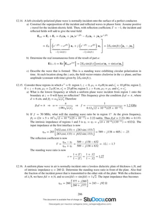
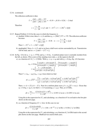
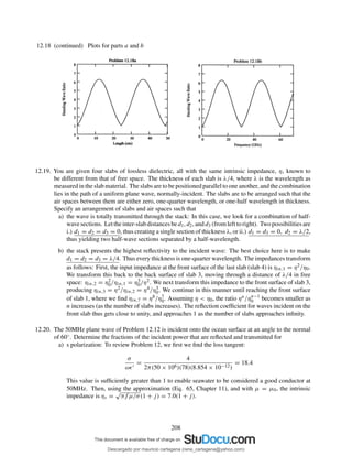
![12.28. Over a certain frequency range, the refractive index of a certain material varies approximately linearly
with frequency: n(ω)
.
= na + nb(ω − ωa), where na, nb, and ωa are constants. Using β = nω/c:
a) determine the group velocity as a function (or perhaps not a function) of frequency:
vg = (dβ/dω)−1, where
dβ
dω
=
d
dω
naω
c
+
nb(ω − ωa)ω
c
=
1
c
[na + nb(2ω − ωa)]
so that
vg(ω) = c [na + nb(2ω − ωa)]−1
b) determine the group dispersion parameter, β2:
β2 =
d2β
dω2 ω0
=
d
dω
1
c
[na + nb(2ω − ωa)]
ω0
= 2nb/c
c) Discuss the implications of these results, if any, on pulse broadening: The point of this problem was
to show that higher order terms (involving d3β/dω3 and higher) in the Taylor series expansion,
Eq. (89), do not exist if the refractive index varies linearly with ω. These higher order terms
would be necessary in cases involving pulses of exremely large bandwidth, or in media exhibiting
complicated variations in their ω-β curves over relatively small frequency ranges. With d2β/dω2
constant, the three-term Taylor expansion of Eq. (89) describes the phase constant of this medium
exactly. The pulse will broaden and will acquire a frequency sweep (chirp) that is precisely linear
with time. Additionally, a pulse of a given bandwidth will broaden by the same amount, regardless
of what carrier frequency is used.
12.29. A T = 5 ps transform-limited pulse propagates in a dispersive channel for which β2 = 10 ps2/km.
Over what distance will the pulse spread to twice its initial width? After propagation, the width is
T ′ = T 2 + ( τ)2 = 2T . Thus τ =
√
3T , where τ = β2z/T . Therefore
β2z
T
=
√
3T or z =
√
3T 2
β2
=
√
3(5 ps)2
10 ps2/km
= 4.3 km
12.30. A T = 20 ps transform-limited pulse propagates through 10 km of a dispersive channel for which β2 =
12 ps2/km. The pulse then propagates through a second 10 km channel for which β2 = −12 ps2/km.
Describe the pulse at the output of the second channel and give a physical explanation for what hap-
pened.
Our theory of pulse spreading will allow for changes in β2 down the length of the channel. In fact, we
may write in general:
τ =
1
T
L
0
β2(z) dz
Having β2 change sign at the midpoint, yields a zero τ, and so the pulse emerges from the output
unchanged! Physically, the pulse acquires a positive linear chirp (frequency increases with time over
the pulse envelope) during the first half of the channel. When β2 switches sign, the pulse begins to
acquire a negative chirp in the second half, which, over an equal distance, will completely eliminate
the chirp acquired during the first half. The pulse, if originally transform-limited at input, will emerge,
again transform-limited, at its original width. More generally, complete dispersion compensation is
achieved using a two-segment channel when β2L = −β′
2L′, assuming dispersion terms of higher order
than β2 do not exist.
212
Descargado por mauricio cartagena (rene_cartagena@yahoo.com)
lOMoARcPSD|5423334](https://image.slidesharecdn.com/solucionario-teoria-electromagnetica-hayt-2001-201211183707/85/Solucionario-teoria-electromagnetica-hayt-2001-214-320.jpg)
![CHAPTER 13
13.1. The parameters of a certain transmission line operating at 6 × 10⁸ rad/s are L = 0.4 µH/m, C =
40 pF/m, G = 80 mS/m, and R = 20 /m.
a) Find γ , α, β, λ, and Z0: We use
γ =
√
ZY = (R + jωL)(G + jωC)
= [20 + j(6 × 10⁸)(0.4 × 10⁻⁶)][80 × 10−3 + j(6 × 10⁸)(40 × 10−12)]
= 2.8 + j3.5 m−1
= α + jβ
Therefore, α = 2.8 Np/m, β = 3.5 rad/m, and λ = 2π/β = 1.8 m. Finally,
Z0 =
Z
Y
=
R + jωL
G + jωC
=
20 + j2.4 × 102
80 × 10−3 + j2.4 × 10−2
= 44 + j30
b) If a voltage wave travels 20 m down the line, what percentage of the original amplitude remains,
and by how many degrees is it phase shifted? First,
V20
V0
= e−αL
= e−(2.8)(20)
= 4.8 × 10⁻²⁵
or 4.8 × 10⁻²³
percent!
Then the phase shift is given by βL, which in degrees becomes
φ = βL
360
2π
= (3.5)(20)
360
2π
= 4.0 × 10³
degrees
13.2. A lossless transmission line with Z0 = 60 is being operated at 60 MHz. The velocity on the line is
3 × 10⁸ m/s. If the line is short-circuited at z = 0, find Zin at:
a) z = −1m: We use the expression for input impedance (Eq. 12), under the conditions Z2 = 60
and Z3 = 0:
Zin = Z2
Z3 cos(βl) + jZ2 sin(βl)
Z2 cos(βl) + jZ3 sin(βl)
= j60 tan(βl)
where l = −z, and where the phase constant is β = 2πc/f = 2π(3 × 10⁸)/(6 × 107) =
(2/5)π rad/m. Now, with z = −1 (l = 1), we find Zin = j60 tan(2π/5) = j184.6 .
b) z = −2 m: Zin = j60 tan(4π/5) = −j43.6
c) z = −2.5 m: Zin = j60 tan(5π/5) = 0
d) z = −1.25 m: Zin = j60 tan(π/2) = j∞ (open circuit)
13.3. The characteristic impedance of a certain lossless transmission line is 72 . If L = 0.5 µH/m, find:
a) C: Use Z0 =
√
L/C, or
C =
L
Z2
0
=
5 × 10⁻⁷
(72)2
= 9.6 × 10⁻¹¹
F/m = 96 pF/m
213
Descargado por mauricio cartagena (rene_cartagena@yahoo.com)
lOMoARcPSD|5423334](https://image.slidesharecdn.com/solucionario-teoria-electromagnetica-hayt-2001-201211183707/85/Solucionario-teoria-electromagnetica-hayt-2001-215-320.jpg)
![13.3b) vp:
vp =
1
√
LC
=
1
(5 × 10⁻⁷)(9.6 × 10⁻¹¹)
= 1.44 × 10⁸
m/s
c) β if f = 80 MHz:
β = ω
√
LC =
2π × 80 × 106
1.44 × 108
= 3.5 rad/m
d) The line is terminated with a load of 60 . Find Ŵ and s:
Ŵ =
60 − 72
60 + 72
= −0.09 s =
1 + |Ŵ|
1 − |Ŵ|
=
1 + .09
1 − .09
= 1.2
13.4. A lossless transmission line having Z0 = 120 is operating at ω = 5 × 10⁸ rad/s. If the velocity on
the line is 2.4 × 10⁸ m/s, find:
a) L: With Z0 =
√
L/C and v = 1/
√
LC, we find L = Z0/v = 120/2.4 × 108 = 0.50 µH/m.
b) C: Use Z0v =
√
L/C/
√
LC ⇒ C = 1/(Z0v) = [120(2.4 × 10⁸)]−1 = 35 pF/m.
c) Let ZL be represented by an inductance of 0.6 µH in series with a 100- resistance. Find Ŵ and
s: The inductive impedance is jωL = j(5 × 10⁸)(0.6 × 10⁻⁶) = j300. So the load impedance
is ZL = 100 + j300 . Now
Ŵ =
ZL − Z0
ZL + Z0
=
100 + j300 − 120
100 + j300 + 120
= 0.62 + j0.52 = 0.808 40◦
Then
s =
1 + |Ŵ|
1 − |Ŵ|
=
1 + 0.808
1 − 0.808
= 9.4
13.5. Two characteristics of a certain lossless transmission line are Z0 = 50 and γ = 0 + j0.2π m−1 at
f = 60 MHz.
a) Find L and C for the line: We have β = 0.2π = ω
√
LC and Z0 = 50 =
√
L/C. Thus
β
Z0
= ωC ⇒ C =
β
ωZ0
=
0.2π
(2π × 60 × 106)(50)
=
1
3
× 1010
= 33.3 pF/m
Then L = CZ2
0 = (33.3 × 10⁻¹²)(50)2 = 8.33 × 10⁻⁸ H/m = 83.3 nH/m.
b) A load, ZL = 60 + j80 is located at z = 0. What is the shortest distance from the load to a
point at which Zin = Rin + j0? I will do this using two different methods:
The Hard Way: We use the general expression
Zin = Z0
ZL + jZ0 tan(βl)
Z0 + jZL tan(βl)
We can then normalize the impedances with respect to Z0 and write
zin =
Zin
Z0
=
(ZL/Z0) + j tan(βl)
1 + j(ZL/Z0) tan(βl)
=
zL + j tan(βl)
1 + jzL tan(βl)
where zL = (60 + j80)/50 = 1.2 + j1.6.
214
Descargado por mauricio cartagena (rene_cartagena@yahoo.com)
lOMoARcPSD|5423334](https://image.slidesharecdn.com/solucionario-teoria-electromagnetica-hayt-2001-201211183707/85/Solucionario-teoria-electromagnetica-hayt-2001-216-320.jpg)
![13.5b. (continued) Using this, and defining x = tan(βl), we find
zin =
1.2 + j(1.6 + x)
(1 − 1.6x) + j1.2x
(1 − 1.6x) − j1.2x
(1 − 1.6x) − j1.2x
The second bracketed term is a factor of one, composed of the complex conjugate of the denomi-
nator of the first term, divided by itself. Carrying out this product, we find
zin =
1.2(1 − 1.6x) + 1.2x(1.6 + x) − j[(1.2)2x − (1.6 + x)(1 − 1.6x)]
(1 − 1.6x)2 + (1.2)2x2
We require the imaginary part to be zero. Thus
(1.2)2
x − (1.6 + x)(1 − 1.6x) = 0 ⇒ 1.6x2
+ 3x − 1.6 = 0
So
x = tan(βl) =
−3 ± 9 + 4(1.6)2
2(1.6)
= (.433, −2.31)
We take the positive root, and find
βl = tan−1
(.433) = 0.409 ⇒ l =
0.409
0.2π
= 0.65 m = 65 cm
The Easy Way: We find
Ŵ =
60 + j80 − 50
60 + j80 + 50
= 0.405 + j0.432 = 0.59 0.818
Thus φ = 0.818 rad, and we use the fact that the input impedance will be purely real at the location
of a voltage minimum or maximum. The first voltage maximum will occur at a distance in front
of the load given by
zmax =
φ
2β
=
0.818
2(0.2π)
= 0.65 m
13.6. The propagation constant of a lossy transmission line is 1 + j2 m−1, and its characteristic impedance
is 20 + j0 at ω = 1 Mrad/s. Find L, C, R, and G for the line: Begin with
Z0 =
R + jωL
G + jωL
= 20 ⇒ R + jωL = 400(G + jωC) (1)
Then
γ 2
= (R + jωL)(G + jωC) = (1 + j2)2
⇒ 400(G + jωC)2
= (1 + j2)2
(2)
where (1) has been used. Eq. 2 now becomes G + jωC = (1 + j2)/20. Equating real and imaginary
parts leads to G = .05 S/m and C = 1/(10ω) = 10−7 = 0.1 µF/m.
215
Descargado por mauricio cartagena (rene_cartagena@yahoo.com)
lOMoARcPSD|5423334](https://image.slidesharecdn.com/solucionario-teoria-electromagnetica-hayt-2001-201211183707/85/Solucionario-teoria-electromagnetica-hayt-2001-217-320.jpg)
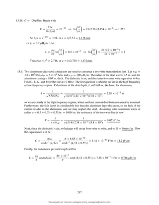
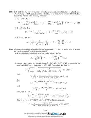
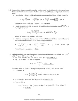
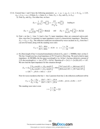
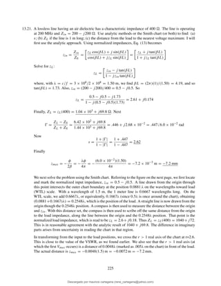
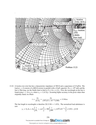
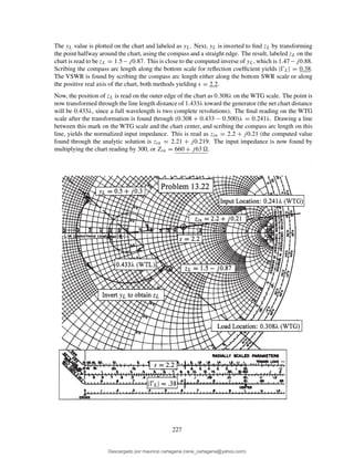
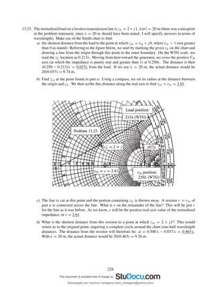
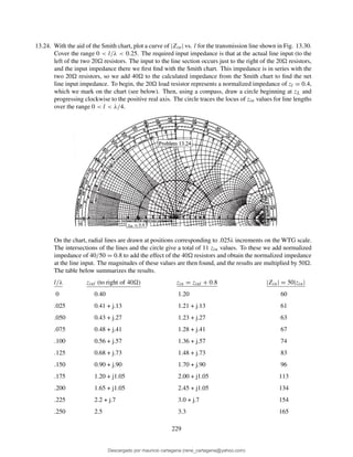
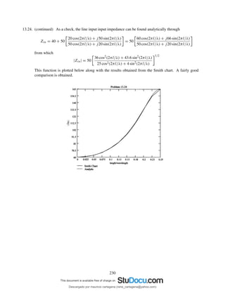
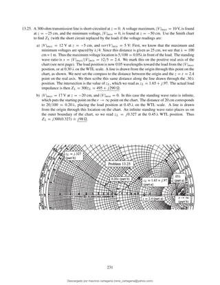
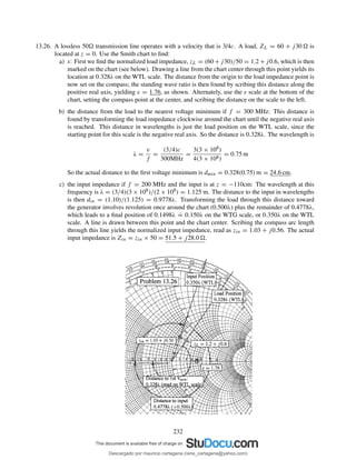
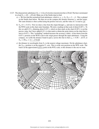
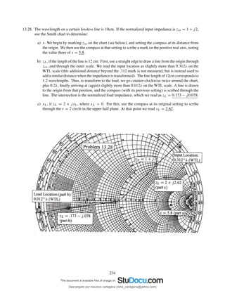
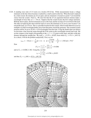
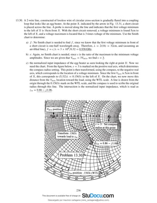
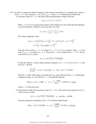
![13.32. A lossless line is operating with Z0 = 40 , f = 20 MHz, and β = 7.5π rad/m. With a short circuit
replacing the load, a minimum is found at a point on the line marked by a small spot of puce paint.
With the load installed, it is found that s = 1.5 and a voltage minimum is located 1m toward the source
from the puce dot.
a) Find ZL: First, the wavelength is given by λ = 2π/β = 2/7.5 = 0.2667m. The 1m distance
is therefore 3.75λ. With the short installed, the Vmin positions will be at multiples of λ/2 to the
left of the short. Therefore, with the actual load installed, the Vmin position as stated would be
3.75λ + nλ/2, which means that a maximum voltage occurs at the load. This being the case, the
normalized load impedance will lie on the positive real axis of the Smith chart, and will be equal
to the standing wave ratio. Therefore, ZL = 40(1.5) = 60 .
b) What load would produce s = 1.5 with |V |max at the paint spot? With |V |max at the paint spot
and with the spot an integer multiple of λ/2 to the left of the load, |V |max must also occur at the
load. The answer is therefore the same as part a, or ZL = 60 .
13.33. In Fig. 13.14, let ZL = 40 − j10 , Z0 = 50 , f = 800 MHz, and v = c.
a) Find the shortest length, d1, of a short-circuited stub, and the shortest distance d that it may be
located from the load to provide a perfect match on the main line to the left of the stub: The Smith
chart construction is shown on the next page. First we find zL = (40 − j10)/50 = 0.8 − j0.2
and plot it on the chart. Next, we find yL = 1/zL by transforming this point halfway around the
chart, where we read yL = 1.17+j0.30. This point is to be transformed to a location at which the
real part of the normalized admittance is unity. The g = 1 circle is highlighted on the chart; yL
transforms to two locations on it: yin1 = 1 − j0.32 and yin2 = 1 + j0.32. The stub is connected
at either of these two points. The stub input admittance must cancel the imaginary part of the line
admittance at that point. If yin2 is chosen, the stub must have input admittance of −j0.32. This
point is marked on the outer circle and occurs at 0.452 λ on the WTG scale. The length of the stub
is found by computing the distance between its input, found above, and the short-circuit position
(stub load end), marked as Psc. This distance is d1 = (0.452−0.250)λ = 0.202 λ. With f = 800
MHz and v = c, the wavelength is λ = (3×10⁸)/(8×108) = 0.375 m. The distance is thus d1 =
(0.202)(0.375) = 0.758 m = 7.6 cm. This is the shortest of the two possible stub lengths, since
if we had used yin1, we would have needed a stub input admittance of +j0.32, which would have
required a longer stub length to realize. The length of the main line between its load and the stub
attachment point is found on the chart by measuring the distance between yL and yin2, in moving
clockwise (toward generator). This distance will be d = [0.500 − (0.178 − 0.138)] λ = 0.46 λ.
The actual length is then d = (0.46)(0.375) = 0.173m = 17.3 cm.
238
Descargado por mauricio cartagena (rene_cartagena@yahoo.com)
lOMoARcPSD|5423334](https://image.slidesharecdn.com/solucionario-teoria-electromagnetica-hayt-2001-201211183707/85/Solucionario-teoria-electromagnetica-hayt-2001-240-320.jpg)
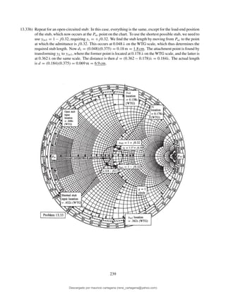
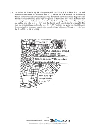
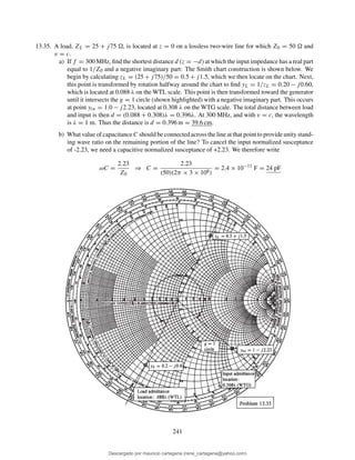
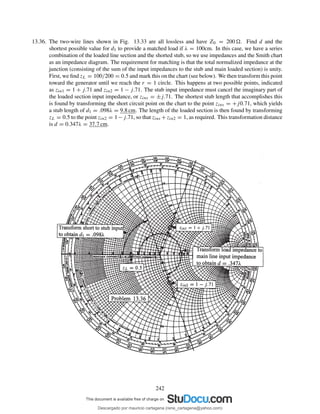
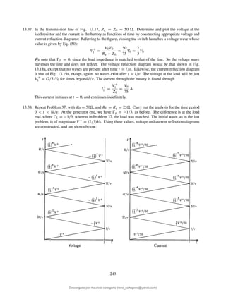
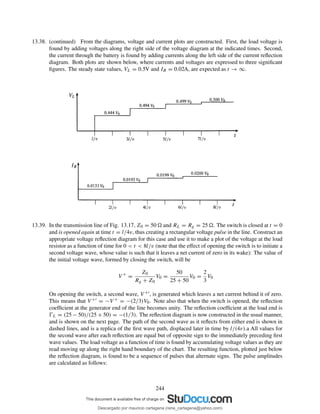
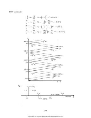
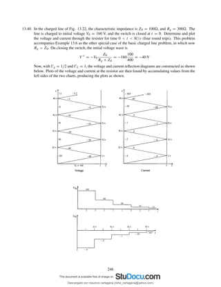
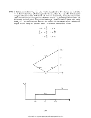
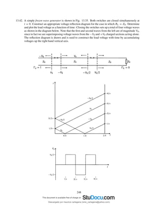
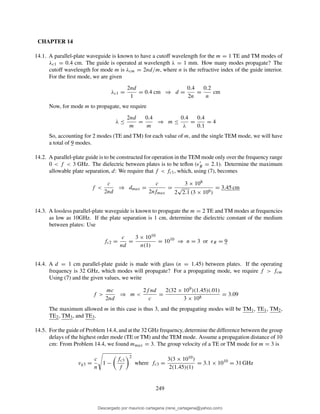
![14.21a. (continued)
Dividing by the magnitude, (0.608)2 + (0.330)2 = 0.692, we obtain the unit vector at t = 0:
aN (0) = −0.879ar + 0.477aθ . We next convert this to cartesian components:
aNx = aN (0) · ax = −0.879 sin θ cos φ + 0.477 cos θ cos φ =
1
√
2
(−0.879 + 0.477) = −0.284
aNy = aN (0) · ay = −0.879 sin θ sin φ + 0.477 cos θ sin φ = 0 since φ = 0
aNz = aN (0) · az = −0.879 cos θ − 0.477 sin θ =
1
√
2
(−0.879 − 0.477) = −0.959
The final result is then
aN (0) = −0.284ax − 0.959az
b) What fraction of the total average power is radiated in the belt, 80◦ < θ < 100◦? We use the
far-zone phasor fields, (84) and (85), and first find the average power density:
Pavg =
1
2
Re[EθsH∗
φs] =
I2
0 d2η
8λ2r2
sin2
θ W/m2
We integrate this over the given belt, an at radius r:
Pbelt =
2π
0
100◦
80◦
I2
0 d2η
8λ2r2
sin2
θ r2
sin θ dθ dφ =
πI2
0 d2η
4λ2
100◦
80◦
sin3
θ dθ
Evaluating the integral, we find
Pbelt =
πI2
0 d2η
4λ2
−
1
3
cos θ sin2
θ + 2
100
80
= (0.344)
πI2
0 d2η
4λ2
The total power is found by performing the same integral over θ, where 0 < θ < 180◦. Doing
this, it is found that
Ptot = (1.333)
πI2
0 d2η
4λ2
The fraction of the total power in the belt is then f = 0.344/1.333 = 0.258.
14.22. Prepare a curve, r vs. θ in polar coordinates, showing the locus in the φ = 0 plane where:
a) the radiation field |Eθs| is one-half of its value at r = 104 m, θ = π/2: Assuming the far field
approximation, we use (84) to set up the equation:
|Eθs| =
I0dη
2λr
sin θ =
1
2
×
I0dη
2 × 10⁴λ
⇒ r = 2 × 10⁴
sin θ
b) the average radiated power density, Pr,av, is one-half of its value at r = 104 m, θ = π/2. To find
the average power, we use (84) and (85) in
Pr,av =
1
2
Re{EθsH∗
φs} =
1
2
I2
0 d2η
4λ2r2
sin2
θ =
1
2
×
1
2
I2
0 d2η
4λ2(108)
⇒ r =
√
2 × 10⁴
sin θ
256
Descargado por mauricio cartagena (rene_cartagena@yahoo.com)
lOMoARcPSD|5423334](https://image.slidesharecdn.com/solucionario-teoria-electromagnetica-hayt-2001-201211183707/85/Solucionario-teoria-electromagnetica-hayt-2001-258-320.jpg)
 = −(1.24 × 10⁻²)(ay + az) V/m.
e) Find |E| at (1000, 0, 0) at t = 0: Taking the magnitude of the part d result, we find |E| =
1.75 × 10⁻² V/m.
257
Descargado por mauricio cartagena (rene_cartagena@yahoo.com)
lOMoARcPSD|5423334](https://image.slidesharecdn.com/solucionario-teoria-electromagnetica-hayt-2001-201211183707/85/Solucionario-teoria-electromagnetica-hayt-2001-259-320.jpg)