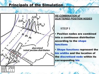
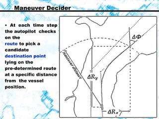
This document summarizes a stochastic modeling study of transit vessel traffic through the Strait of Istanbul. The objectives were to quantify casualty risk variation based on vessel size and different regions of the Strait. A mathematical simulation was developed using stochastic parameters like vessel length and pilot error. Position distributions were evaluated along checklines. Collision and grounding risks were highest for certain regions and supported statistical data. Further improvements could incorporate more detailed hydrodynamics and bathymetry.

1. Stochastic Modeling of
Transit Vessel Traffic
through the
Strait of Istanbul
Safak Ozkan
Photo: Paul Work
Department of Civil Engineering
Bosphorus University

2. OBJECTIVES:
• to quantify casualty risk
variation…
1)…along the Strait
2)…among different vessel sizes
SCOPE:
• Pilotage errors
• Currents are assumed to be the
predominant factor for vessel
drift
• Vessel lengths are limited to 50
- 200 m
Present Study

3. the Strait of İstanbul
• exchange of two distinct water
systems between BLACK SEA –
MEDDITERANEAN SEA

4. the simulation program rather acts like a
numerical test in order to quantify the casualty
risk relatively
Present Study
METHODOLOGY:
• Stochastic Model
• Random parameters include
LOA and pilotage error
• the autopilot
• Physics Based Mathematical
Simulation

5. • 12 maneuver points
• the turn angles are
@ Üsküdar, Ortaköy and
Büyükdere ∼ 45o
@ Yeniköy ∼ 80o
• At Kandilli and Yeniköy the
forward sight is blocked by
the bends
• Currents mount up to
7-8 knots whilst northerly
winds
• narrowest section at Kandilli
(app. 700 m)
courtesy of Yüce, 1995
Physical Characteristics of the Strait

6. Hydrodynamics of the Strait
• Count Marsigli
identified a two layer
flow in the Strait in
year 1679
• The surface flow is
driven by sea-level
differences, Δη
• The lower layer flow
is driven by density
differences,
ρMed – ρBS
Courtesy of London Science Museum, Photo: Emre Otay

7. Department of Navigation, Hydrography and Oceanography, map no 9001
Surface Currents
(Akyarlı and Arısoy, 1994)
• Quantitative observations on sea
level differences being made since
1918
• mean(Δη) ~ 30 – 35 cm (Büyükay, 1990)
• Instantaneous difference -5 cm to
77 cm. (Akyarlı, 1997)
• transient changes in Δη, and
winds causes orkoz currents be
formed.

8. (Örs, 1998)
Surface Currents
Department of Navigation, Hydrography and Oceanography, map no 9001
MODEL:
• Shallow water equations
• Slip boundary conditions at
the solid boundaries
• Reynolds number is
artificially lowered (Laminar
flow)
REALITY:
• Transient nature
• Under certain
circumstances north-
going counter
currents may develop
(orkoz).

9. Casualty Statistics
• over 300 vessels
involved in
casualties
• Annually 50,000
vessels transit
the Strait
• 10% of them are
tankers with liquid
cargo
• Approximately
every 12 minutes a
vessel enters the
Strait
(Gören, 2002)

10. Present Regulations
• Traffic Separation
Scheme issued in 1994
• Maximum speed
10 knots
• Vessels longer than
200 m cannot keep
within the lanes
• For vessels longer than
300 m, opposite direction
is suspended for all
vessel types
Therefore vessels longer than 200
m are out of the scope of the
present study

11. Ship Hydrodynamics
• ship motion is
represented with 3 DOF
xDp RmFF xx
=+
yDp RmFF yy
=+
zzcurrh IMM φ=+/
Hydrodynamic forces on ship parts are
analyzed separately :
• Hull forces
• Propeller forces
• Rudder forces

12. Equations of Motion
∫ ∫
+
⎥
⎥
⎦
⎤
⎢
⎢
⎣
⎡
+
+
=Δ
Tt
t
ox
t
t
Dpx
x
o
o o
x
dttRdt
m
tFtF
R )(
)()(
∫ ∫
+
⎥
⎥
⎦
⎤
⎢
⎢
⎣
⎡
+
+
=Δ
Tt
t
oy
t
t
Dpy
y
o
o o
y
dttRdt
m
tFtF
R )(
)()(
∫ ∫
+
⎥
⎥
⎦
⎤
⎢
⎢
⎣
⎡
+
+
=Δ
Tt
t
oz
t
t
currh
z
o
o o
dttdt
m
tMtM
)(
)()(/
φφ
xDp RmFF xx
=+
yDp RmFF yy
=+
zzcurrh IMM φ=+/

13. Hull Forces
• Hull forces are computed along
the longitudinal axis and
transverse axis of the vessel
• The empirical equations are
suitable for maneuvering vessels
at low velocities.
• Hull forces are due to viscous drag
and lift forces
tctvt eVVYF ,)( φ⋅−=
φφρ eeVVACCF ctwsrfl ⋅⋅−+−=
2
2
1 )()(

14. • Propeller thrust is set constant
such that the linear velocity of the
vessel is around 10 knots during the
navigation
• For southbound vessels, calm water
velocity is 8 knots
• For southbound vessels, calm water
velocity is 12 knots
LOAsouthbound=125 m, complete navigation
Propeller Forces

15. courtesy of Schilling Rudder Systems
• Rudder is a
symmetrical hydrofoil
shadowed by the hull
augmented by the
propeller
• Force developed on
rudder is proportional
to square of the inflow
velocity
Rudder Forces
2
nflowiL UF ∝

16. Rudder Forces
courtesy of Schilling Rudder Systems
• FL results in a turning moment
on the hull
• At stall point CL is maximum
• Conventional rudders have stall
angles at 35o
• Beyond the stall point CL

17. Photo: Conny Wickberg
Ship Maneuverability
Turning Circle Test:
A measurement of
ship maneuverability

18. Turning Circle Test
925 m965 m
Tactical
Diameter
360 m394 mTransfer
1015 m1068 mAdvance
Real
Parameters
(ESSO
OSAKA)
Simulation
– simulation –
IMO specifications (2002) on ship
maneuverability require that the
turning circle parameters be
linearly related to vessel length

19. • The Strait is meshed
with stations into 10
sub-regions where major
course alterations take
place.
• Navigation runs are
carried out in between
every two successive
stations separately.
• Regions are meshed
with checklines
• Vessel positions are
recorded where their
Principals of the Simulation

20. ASSUMPTIONS & METHODOLOGY:
• Main philosophy is to evaluate the
mapping of the position distributions
from one checkline to the next
• Vessels are handled by an
autopilot
• The autopilot acts with a constant
level of error in a region of course
alteration
• Surface current includes no eddies
• Constant currents act at all points
around the ship hull
• The navigation of vessels is
independent of the opposite
direction traffic.
Principals of the Simulation

21. RANDOM VARIABLES:
• vessel length f(LOA),
all the vessel related parameters are related to
LOA
Principals of the Simulation
• initial position f(xin)
• autopilot error parameters
f(ε ), f(τ )

22. Principals of the Simulation
DISCRETIZATION of the INPUT
VARIABLES:
• Initial conditions, , are
correlated to xin by curve fitting)
• Whenever a random distribution is
discretized, the shape of the
distribution within the discretized bin
is approximated with a constant
shape function

23. Principals of the Simulation
RE-COMBINATION of
SCATTERED POSITION NODES:
• the set of discrete position
nodes have to be drawn back
into a continuous form at the
entrance of a navigation region
• When the navigation run is
completed we have a set of
discrete position points
scattered along the line
(checkline or station)
• this is achieved in two steps

24. Principals of the Simulation
RE-COMBINATION of
SCATTERED POSITION NODES:
STEP 1
• Since the pilotage error is
originally a continuous
distribution, the position nodes
originating from one single
initial vessel represents a
continuous distribution on the
checkline

25. Principals of the Simulation
RE-COMBINATION of
SCATTERED POSITION NODES:
STEP 1
• Position nodes are combined
into a continuous distribution
according to the shape
functions
• Shape functions represent the
bin widths and the location of
the discretised node within its
corresponding bin

26. Principals of the Simulation
RE-COMBINATION of
SCATTERED POSITION NODES
STEP 2
• In the end we have a number
of continuous position
distributions – for each initial vessel
position – to be composed into
the ultimate position
distribution

27. Routes According to TSS
• Routes are developed by
locating the mid-lines of the
TSS lanes
• All vessel sizes
incorporated in the
program, i.e.
(50 m < LOA < 200 m)
are assumed to follow the
same pre-determined
routes

28. • At each time step
the autopilot checks
on the
route to pick a
candidate
destination point
lying on the
pre-determined route
at a specific distance
from the vessel
position.
Maneuver Decider

29. Maneuver Decider
• When an
isosceles triangle
is formed
between vessel
position and
destination point
maneuver is
initiated
• The autopilot is
provided with the
constraint
variables
ΔRx ΔRy and Δφz

30. Autopilot
∫ ∫
+
⎥
⎥
⎦
⎤
⎢
⎢
⎣
⎡
+
+
=Δ
Tt
t
ox
t
t
Dp
x
o
o o
xx
dttRdt
m
tFtF
R )(
)()(
∫ ∫
+
⎥
⎥
⎦
⎤
⎢
⎢
⎣
⎡
+
+
=Δ
Tt
t
oy
t
t
Dp
y
o
o o
yy
dttRdt
m
tFtF
R )(
)()(
∫ ∫
+
⎥
⎥
⎦
⎤
⎢
⎢
⎣
⎡
+
+
=Δ
Tt
t
oz
t
t
currp
z
o
o o
dttdt
m
tMtM
)(
)()(/
φφ
• The autopilot physically
has the control of the
rudder angle, γ (t)
• There are 3 constraint
equations to be satisfied
• Therefore a physical
model for γ (t) must be
constructed which must
bring in only 3 unknowns.

31. ( )2
21
2
22 TTTTl o Δ−Δ−
+
=Δ+
γγ
γ
( )2
21
1
1 TTTTl oo Δ−Δ−
+
=Δ+
γγ
γ
• The physical model for γ`(t)
is a partially defined function
which includes
only 3 unknowns:
γ1 , γ2 , T
a Physical Model for γ (t)

32. • 3 equations – 3 unknowns
• the equations are implicit
integral equations
• discretization of the
equations yield non-linear
terms
• Newton-Raphson method is
used
a Physical Model for γ (t)
∫ ∫
+
⎥
⎥
⎦
⎤
⎢
⎢
⎣
⎡
+
+
=Δ
Tt
t
ox
t
t
Dp
x
o
o o
xx
dttRdt
m
tFtF
R )(
)()(
∫ ∫
+
⎥
⎥
⎦
⎤
⎢
⎢
⎣
⎡
+
+
=Δ
Tt
t
oy
t
t
Dp
y
o
o o
yy
dttRdt
m
tFtF
R )(
)()(
∫ ∫
+
⎥
⎥
⎦
⎤
⎢
⎢
⎣
⎡
+
+
=Δ
Tt
t
oz
t
t
currp
z
o
o o
dttdt
m
tMtM
)(
)()(/
φφ
Equations:
Unknowns:
γ1
γ2
T

33. Human errors are primarily
classified in two categories
• lack of ship-handling skills
• lack of knowledge
(Poyraz and Paksoy, 1998; Oğuzülgen 1995)
• ε, (handling error),
set γ(t) = ε ⋅ γ`(t)
• τ, (delay error),
during the computations of γ`(t),
the magnitude and the direction
of surface currents are
perceived with a time delay
Autopilot Error Parameters τ and ε
perfect pilotage corresponds to ε =
100%, τ = 0 sec.

34. pure handling, ε , and
pure delay, τ , errors

35. Position Distributions
• All the
simulation
program does is
evaluate the
probability
distributions of
vessels along the
checklines
• The casualty
risks are
evaluated
afterwards in a
post-processing

36. Ramming and Grounding
INPUT:
• Q=50,000 vessels/year
• f(LOA)
Investigate the casualty risk
variation
• vessel length, LOA
• travel direction
• casualty type
• regions of the Strait

37. Casualty Model – Collision Risk
x
{ } dxXxSdxXxN SN
)()(∫ ∫=ξ
groundingzone
collision
zone
2
Q∝ξ

38. Casualty Model – Collision Risk
High risk regions are
(simulation)
•Yeniköy
•Büyükdere – Sarıyer
•Kandilli

39. Casualty Model – Ramming and Grounding
groundingzone
∫=Λ dxXxN N
)(
Q∝Λ

40. Casualty Model – Ramming and Grounding
High risk regions are
(simulation)
•Ortaköy – Kanlıca

41. Comparison with Statistical Data
• Collision risk is overestimated for larger
vessels (Probably due to better ship-handling provided
for larger vessels)
– simulation –
– statistical data –
(Gören, 2002)

42. Comparison with Statistical Data
(Gören, 2002)
SIMULATION:
31.1≅
Λ
ξ
MEASURED:
95.1≅
Λ
ξ
• R/G seem to be
over-estimated
(Error is primarily due
to constant shape
functions)

43. Conclusion
• CRG risk is evaluated with stochastic simulation
• southbound vessels are at a more disadvantageous
situation in terms of rudder control
• vessel lengths directly correlate with CRG risk
• High risk regions: Yeniköy, Kandilli and Büyükdere
• Collision risk is higher than R/G risk
• ξ ∝ Q2
• Λ ∝ Q

44. • Higher order shape functions must be
incorporated
• Different routes lying within the TSS lanes may
be incorporated
• Water currents be solved numerically as a
function of Δη and ρMed – ρBS
• Ship hydrodynamic forces be elaborated to
include the shallow water and narrow channel
effects
• A detailed bathymetry data can be supplied for
better representation of grounding zones for
Further Improvements of the Simulation

45. Future Prospects Offered by This Study
• Real time simulations can be
implemented with extensive
simultaneous surface current
measurements
• Similar channels can be
analyzed with this mathematical
simulation program for
quantitative risk level
comparison with the Strait of
İstanbul