Unsupervised Machine Learning PPT Adi.pdf

Unsupervised
Learning and
Association Mining Introduction
Clustering Types
K-Means algorithm
Association Mining
FP-growth
2
Clustering
Contents--
Prof. Dr. K. Adisesha

Introduction
3
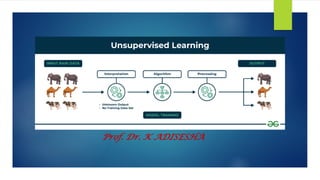
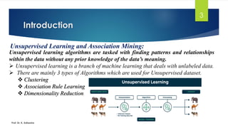
Unsupervised Learning and Association Mining:
Unsupervised learning algorithms are tasked with finding patterns and relationships
within the data without any prior knowledge of the data’s meaning.
➢ Unsupervised learning is a branch of machine learning that deals with unlabeled data.
➢ There are mainly 3 types of Algorithms which are used for Unsupervised dataset.
❖ Clustering
❖ Association Rule Learning
❖ Dimensionality Reduction

Unsupervised Learning
4
Clustering Algorithms:
Clustering in unsupervised machine learning is the process of grouping unlabeled data
into clusters based on their similarities.
➢ The goal of clustering is to identify patterns and relationships in the data without any
prior knowledge of the data’s meaning.
➢ Some common clustering algorithms:
❖ Hierarchical Clustering: Creates clusters by building a tree step-by-step, either merging or splitting
groups.
❖ K-means Clustering: Groups data into K clusters based on how close the points are to each other.
❖ Density-Based Clustering (DBSCAN): Finds clusters in dense areas and treats scattered points as noise.
❖ Mean-Shift Clustering: Discovers clusters by moving points toward the most crowded areas.
❖ Probalistic clustering: Clusters are created using probability distribution.

5
Association Rule Learning:
Association rule learning is also known as association rule mining is a common
technique used to discover associations in unsupervised machine learning.
➢ This technique is a rule-based ML technique that finds out some very useful relations
between parameters of a large data set.
➢ Some common Association Rule Learning algorithms:
❖ Apriori Algorithm: Finds patterns by exploring frequent item combinations step-by-step.
❖ FP-Growth Algorithm: An Efficient Alternative to Apriori. It quickly identifies frequent
patterns without generating candidate sets.
❖ Eclat Algorithm: Uses intersections of itemsets to efficiently find frequent patterns.
❖ Efficient Tree-based Algorithms: Scales to handle large datasets by organizing data in tree
structures.

6
Dimensionality Reduction:
Dimensionality reduction is the process of reducing the number of features in a dataset
while preserving as much information as possible.
➢ Here are some popular Dimensionality Reduction algorithms:
❖ Principal Component Analysis (PCA): Reduces dimensions by transforming data into
uncorrelated principal components.
❖ Linear Discriminant Analysis (LDA): Reduces dimensions while maximizing class separability
for classification tasks.
❖ Non-negative Matrix Factorization (NMF): Breaks data into non-negative parts to simplify
representation.
❖ Isomap: Captures global data structure by preserving distances along a manifold.

7
Challenges of Unsupervised Learning:
Here are the key challenges of unsupervised learning:
➢ Noisy Data: Outliers and noise can distort patterns and reduce the effectiveness of
algorithms.
➢ Assumption Dependence: Algorithms often rely on assumptions (e.g., cluster shapes),
which may not match the actual data structure.
➢ Overfitting Risk: Overfitting can occur when models capture noise instead of
meaningful patterns in the data.
➢ Limited Guidance: The absence of labels restricts the ability to guide the algorithm
toward specific outcomes.
➢ Cluster Interpretability: Results, such as clusters, may lack clear meaning or alignment
with real-world categories.

8
Applications of Unsupervised learning:
Unsupervised learning has diverse applications across industries and domains. Key
applications include:
➢ Customer Segmentation: Algorithms cluster customers based on purchasing behavior or
demographics, enabling targeted marketing strategies.
➢ Anomaly Detection: Identifies unusual patterns in data, aiding fraud detection, cybersecurity,
and equipment failure prevention.
➢ Recommendation Systems: Suggests products, movies, or music by analyzing user behavior and
preferences.
➢ Image and Text Clustering: Groups similar images or documents for tasks like organization,
classification, or content recommendation.
➢ Social Network Analysis: Detects communities or trends in user interactions on social media
platforms.

Clustering Models
9
Hierarchical vs Non-Hierarchical Clustering:
Two commonly utilized clustering approaches are Hierarchical Clustering and
Non−Hierarchical Clustering.
➢ Hierarchical Clustering may be a flexible clustering method that makes various levelled
structures of clusters. It can be performed utilizing two primary strategies:
❖ Agglomerative progressive clustering
❖ Divisive progressive clustering
➢ Non-Hierarchical Clustering: also known as partition clustering, points to
straightforwardly relegating information focuses to clusters without considering a
progressive structure.
➢ It incorporates well−known calculations such as K−means, DBSCAN, and Gaussian Blend
Models (GMM).

Clustering Models
10
Hierarchical vs Non-Hierarchical Clustering:
Two commonly utilized clustering approaches are Hierarchical Clustering and
Non−Hierarchical Clustering.
➢ Hierarchical Clustering
➢ Non-Hierarchical Clustering:

Clustering Models
11
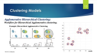
Agglomerative Hierarchical Clustering:
Agglomerative Hierarchical clustering is a bottom-up clustering approach where
clusters have sub-clusters, which consecutively have sub-clusters, etc.
➢ It is also known as the bottom-up approach or hierarchical agglomerative clustering
(HAC).
➢ Unlike flat clustering hierarchical clustering
provides a structured way to group data.
➢ This clustering algorithm does not require us
to prespecify the number of clusters.

Clustering Models
12
Workflow for Hierarchical Agglomerative clustering.
1. Start with individual points: Each data point is its own cluster. For example if you have 5 data points
you start with 5 clusters each containing just one data point.
2. Calculate distances between clusters: Calculate the distance between every pair of clusters. Initially
since each cluster has one point this is the distance between the two data points.
3. Merge the closest clusters: Identify the two clusters with the smallest distance and merge them into a
single cluster.
4. Update distance matrix: After merging you now have one less cluster. Recalculate the distances between
the new cluster and the remaining clusters.
5. Repeat steps 3 and 4: Keep merging the closest clusters and updating the distance matrix until you have
only one cluster left.
6. Create a dendrogram: As the process continues you can visualize the merging of clusters using a tree-
like diagram called a dendrogram. It shows the hierarchy of how clusters are merged.

Clustering Models
13

Clustering Models
14
Hierarchical Divisive clustering:
It is also known as a top-down approach. This algorithm also does not require to
prespecify the number of clusters.
➢ Top-down clustering requires a method for splitting a cluster that contains the whole
data and proceeds by splitting clusters recursively until individual data have been split
into singleton clusters.

Clustering Models
15
1. Start with all data points in one cluster: Treat the entire dataset as a single large cluster.
2. Split the cluster: Divide the cluster into two smaller clusters. The division is typically done
by finding the two most dissimilar points in the cluster and using them to separate the data
into two parts.
3. Repeat the process: For each of the new clusters, repeat the splitting process:
❖ Choose the cluster with the most dissimilar points.
❖ Split it again into two smaller clusters.
4. Stop when each data point is in its own cluster: Continue this process until every data
point is its own cluster, or the stopping condition (such as a predefined number of clusters)
is met.

Clustering Models
16

Clustering Models
17
Computing Distance Matrix:
While merging two clusters we check the distance between two every pair of clusters
and merge the pair with the least distance/most similarity.
➢ But the question is how is that distance determined.
➢ There are different ways of defining Inter Cluster distance/similarity. Some of them
are:

Clustering Models
18
Computing Distance Matrix:
While merging two clusters we check the distance between two every pair of clusters
and merge the pair with the least distance/most similarity.
➢ But the question is how is that distance determined.
➢ There are different ways of defining Inter Cluster distance/similarity. Some of them
are:
❖ Min Distance: Find the minimum distance between any two points of the cluster.
❖ Max Distance: Find the maximum distance between any two points of the cluster.
❖ Group Average: Find the average distance between every two points of the clusters.
❖ Ward’s Method: The similarity of two clusters is based on the increase in squared
error when two clusters are merged.

Clustering Models
19
K-means Clustering:
K-means clustering is an unsupervised learning algorithm used for data clustering,
which groups unlabeled data points into groups or clusters.
➢ For example, online store uses K-Means to group customers based on purchase
frequency and spending creating segments personalised marketing.
➢ The algorithm works by first randomly picking some
central points called centroids and each data point is
then assigned to the closest centroid forming a cluster.
➢ After all the points are assigned to a cluster the
centroids are updated by finding the average position of
the points in each cluster.

Clustering Models
20
K-means Clustering:
The algorithm will categorize the items into k groups or clusters of similarity. To
calculate that similarity, we will use the Euclidean distance as a measurement.
➢ The algorithm works as follows:
❖ First, we randomly initialize k points, called means or cluster centroids.
❖ We categorize each item to its closest mean, and
we update the mean’s coordinates, which are the
averages of the items categorized in that cluster so
far.
❖ We repeat the process for a given number of
iterations and at the end, we have our clusters.

Clustering Models
21
K-means Clustering:
The algorithm will categorize the items into k groups or clusters of similarity.
➢ First, we randomly initialize k points, called means or cluster centroids.
➢ Given a set of observations (x1, x2, ..., xn), where each observation is a d-dimensional
real vector, k-means clustering aims to partition the n observations into k (≤ n) sets
S = {S1, S2, ..., Sk} so as to minimize the within-cluster sum of
squares (variance). Formally, the objective is to find:
where μi is the mean (also called centroid) of points in Si, i.e.

Clustering Models
22
K-means Clustering:
The goal of the K-Means algorithm is to find clusters in the given input data. The
flowchart below shows how k-means clustering works:
➢ The goal of the K-Means algorithm is to find clusters in the given input data.

Clustering Models
23
K-means Clustering Method:
Example

Clustering Models
24
K-means Clustering:
K-means Clustering – Details
➢ Initial centroids are often chosen randomly.
❖Clusters produced vary from one run to another.
➢ The centroid is (typically) the mean of the points in the cluster.
➢ ‘Closeness’is measured by Euclidean distance, cosine similarity, correlation, etc.
➢ K-means will converge for common similarity measures mentioned above.
➢ Most of the convergence happens in the first few iterations.
❖Often the stopping condition is changed to ‘Until relatively few points change clusters’
➢ Complexity is O( n * K * I * d )
❖n = number of points, K = number of clusters, I = number of iterations, d = number of
attributes

Clustering Models
25
Evaluating K-means Clusters:
Most common measure is Sum of Squared Error (SSE)
➢ For each point, the error is the distance to the nearest cluster
➢ To get SSE, we square these errors and sum them.
➢ x is a data point in cluster Ci and mi is the representative point for cluster Ci
❖can show that mi corresponds to the center (mean) of the cluster
➢ Given two clusters, we can choose the one with the smallest error
➢ One easy way to reduce SSE is to increase K, the number of clusters
❖A good clustering with smaller K can have a lower SSE than a poor clustering with higher K

= 
=
K
i C
x
i
i
x
m
dist
SSE
1
2
)
,
(

Clustering Models
26
Evaluating K-means Clusters:
Most common measure is Sum of Squared Error (SSE)
-2 -1.5 -1 -0.5 0 0.5 1 1.5 2
0
0.5
1
1.5
2
2.5
3
x
y
Iteration 6

Clustering Models
27
Limitations of K-means:
K-means has problems when clusters are of differing
❖ Sizes
❖ Densities
❖ Non-globular shapes
➢ K-means has problems when the data contains
outliers.

Clustering Models
28
K-Medoids clustering:
The k-medoids problem is a clustering problem similar to k-means. The name was
coined by Leonard Kaufman and Peter J. Rousseeuw with their PAM (Partitioning
Around Medoids) algorithm.
➢ K-medoids is a classical partitioning technique of clustering
that splits the data set of n objects into k clusters, where the
number k of clusters assumed known a priori.
➢ In K-medoids instead of using centroids of clusters, actual
data points are use to represent clusters.

Clustering Models
29
K-Medoids clustering Algorithm:
The partitioning will be carried on such that each cluster must have at least one object
and an object must belong to only one cluster.

Clustering Models
30
K-medoids:
Applications:
➢ Academic Performance: Based on the scores obtained by the student, they are classified
into grades like A, B, C, D etc.
➢ Diagnostic System: In the medical profession, it helps in creating smarter medical
decision support systems, especially in the treatment of liver ailments.
➢ Document Classification: Cluster documents in multiple categories based on their tags,
topics, and the content of the document.
➢ Customer Segmentation: It helps marketers to improve their customer base, work on
target areas and segment customer based on purchase history, interest. The
classification would help the company target specific clusters of customers for specific
campaigns and sell their products according to their interest.

K-Means K-Medoids
Attempts to minimize the total squared
error.
D Minimizes the sum of dissimilarities between points
labelled to be in A cluster and their closest selected
object.
Takes means of elements in a dataset Takes medoids of elements in a dataset
Time complexity is O(ndk+1) Time complexity is O(k*(n-k)2)
More sensitive to outliners Less sensitive to outliners
Uses Euclidean Distance Uses Partitioning Around Medoids (PAM)
Clustering Models
31
K-means vs K-medoids:
K-Medoid is more efficient as it is less sensitive to outliners which makes it better than
the K-Means method and it is applicable in various fields and in future, it can rise.

Association Rule Learning
32
Association rule learning is a type of unsupervised learning technique that checks for
the dependency of one data item on another data item and maps accordingly so that it
can be more profitable.
➢ The association rule learning is employed in Market Basket analysis, Web usage
mining, continuous production, etc.
➢ For example, if a customer buys bread, he most likely can also buy butter, eggs, or milk,
so these products are stored within a shelf or mostly nearby.

33
Association rule learning works on the concept of If and Else Statement, such as if A
then B.
➢ Here the If element is called antecedent, and then statement is called as Consequent.
➢ Association rule learning can be divided into three types of algorithms:
❖ Apriori: It is mainly used for market basket analysis and helps to understand the products
that can be bought together.
❖ Eclat: Eclat algorithm stands for Equivalence Class Transformation. This algorithm uses a
depth-first search technique to find frequent itemsets in a transaction database.
❖ F-P Growth Algorithm: It stands for Frequent Pattern, and it represents the database in the
form of a tree structure that is known as a frequent pattern or tree.

34
Association rule learning works on the concept of If and Else Statement, such as if A
then B.
➢ to measure the associations between thousands of data items, there are several metrics.
These metrics are given below:
❖ Support: Support is the frequency of A or how frequently an item appears in the
dataset.
❖ Confidence: It is the ratio of the transaction that contains X and Y to the number of
records that contain X.
❖ Lift: It is the ratio of the observed support measure and expected support if X and Y
are independent of each other.

35
Apriori Algorithm:
The Apriori algorithm is a machine learning algorithm that finds frequent patterns in
data. It's used to identify associations between items and create rules based on those
associations.
➢ Apriori Algorithm is a foundational method in data mining used for discovering
frequent item sets and generating association rules.
➢ Its significance lies in its ability to identify relationships between items in large datasets
which is particularly valuable in market basket analysis.
➢ For example, if a grocery store finds that customers who buy bread often also buy
butter, it can use this information to optimize product placement or marketing
strategies.

36
Apriori Algorithm:
The Apriori Algorithm operates through a systematic process that involves several key
steps:
➢ Identifying Frequent Itemsets: The algorithm begins by scanning the dataset to identify
individual items (1-item) and their frequencies.
➢ Creating Possible item group: Once frequent 1-itemgroup(single items) are identified, the
algorithm generates candidate 2-itemgroup by combining frequent items.
➢ Removing Infrequent Item groups: The algorithm employs a pruning technique based on the
Apriori Property, which states that if an itemset is infrequent, all its supersets must also be
infrequent.
➢ Generating Association Rules: After identifying frequent itemsets, the algorithm generates
association rules that illustrate how items relate to one another, using metrics like support,
confidence, and lift to evaluate the strength of these relationships.

37
Apriori Algorithm:
Example of the Apriori Algorithm: Min support 2
➢ Data in the database
➢ Calculate the support/frequency of all items
➢ Discard the items with minimum support less than 2
➢ Combine two items
➢ Calculate the support/frequency of all items
➢ Discard the items with minimum support less than 2.
Combine three items and calculate their support.
➢ Discard the items with minimum support less than 2
Result:
Only one itemset is frequent (Eggs, Tea, Cold Drink)
because this itemset has minimum support 2

38
Apriori Algorithm:
Advantages of Apriori Algorithm:
➢ Apriori Algorithm is the simplest and easy to understand the algorithm for mining the frequent
itemset.
➢ Apriori Algorithm is fully supervised so it does not require labeled data.
➢ Apriori Algorithm is an exhaustive algorithm, so it gives satisfactory results to mine all the
rules within specified confidence and sport.
➢ Apriori principles Downward closure property of frequent patterns which, means that All
subset of any frequent itemset must also be frequent.

39
Eclat Algorithm:
Eclat algorithm stands for Equivalence Class Transformation. This algorithm uses a
➢ Here’s how it works step by step:
❖ Transaction Database: Eclat starts with a transaction database, where each row represents a transaction,
and each column represents an item.
❖ Itemset Generation: Initially, Eclat creates a list of single items as 1-itemsets. It counts the support
(frequency) of each item in the database by scanning it once.
❖ Building Equivalence Classes: Eclat constructs equivalence classes by grouping transactions that share
common items in their 1-itemsets.
❖ Recursive Search: Eclat recursively explores larger itemsets by combining smaller ones. It does this by
taking the intersection of equivalence classes of items.
❖ Pruning: Eclat prunes infrequent itemsets at each step to reduce the search space, just like Apriori.

40
Eclat Algorithm:
➢ Let’s say you have a transactional dataset for a grocery store:
1: {Milk, Bread, Eggs}
2: {Milk, Bread, Diapers}
3: {Milk, Beer, Chips}
4: {Bread, Diapers, Beer, Chips}
5: {Bread, Eggs, Beer}
❖ Suppose you want to find frequent itemsets with a minimum support of 2 transactions.
❖ Initially, the 1-itemsets are {Milk}, {Bread}, {Eggs}, {Diapers}, {Beer}, {Chips}.
❖ Calculate their support.

41
Eclat Algorithm:
❖ Construct equivalence classes:
{Milk}: Transaction 1, 2, 3
{Bread}: Transaction 1, 2, 4, 5
{Eggs}: Transaction 1, 5
❖ Recursively generate larger itemsets:
{Milk, Bread}, {Milk, Eggs}, {Milk, Diapers}, {Milk, Beer}, {Milk, Chips},
{Bread, Eggs}, {Bread, Diapers}, {Bread, Beer}, {Bread, Chips}, {Eggs, Diapers},
{Eggs, Beer}. {Diapers, Beer}, {Diapers, Chips},{Beer, Chips}
❖ Prune itemsets with support less than 2.
❖ Continue this process until no more frequent itemsets can be found.
{Diapers}: Transaction 2, 4
{Beer}: Transaction 3, 4, 5
{Chips}: Transaction 3, 4

42
Eclat Algorithm:
➢ This vertical approach of the ECLAT algorithm makes it a faster algorithm than the Apriori
algorithm.
➢ Transactions, originally stored in horizontal format, are read from disk and converted to
vertical format.

43
Eclat Algorithm:
Example:- Consider the following transactions record:-, minimum support = 2
k=1 k=2
Item Tidset
Bread {T1, T4, T5, T7, T8, T9}
Butter {T1, T2, T3, T4, T6, T8, T9}
Milk {T3, T5, T6, T7, T8, T9}
Coke {T2, T4}
Jam {T1, T8}
Item Tidset
{Bread, Butter} {T1, T4, T8, T9}
{Bread, Milk} {T5, T7, T8, T9}
{Bread, Coke} {T4}
{Bread, Jam} {T1, T8}
{Butter, Milk} {T3, T6, T8, T9}
{Butter, Coke} {T2, T4}
{Butter, Jam} {T1, T8}
{Milk, Jam} {T8}

44
Eclat Algorithm:
Example:- Consider the following transactions record:-, minimum support = 2
k=3 k=4
Item Tidset
{Bread, Butter, Milk} {T8, T9}
{Bread, Butter, Jam} {T1, T8}
Item Tidset
{Bread, Butter,
Milk, Jam}
{T8}
Items Bought Recommended Products
Bread Butter
Bread Milk
Bread Jam
Butter Milk
Butter Coke
Butter Jam
Bread and Butter Milk
Bread and Butter Jam
We stop at k = 4 because there are no more item-tidset pairs to
combine.
Since minimum support = 2, we conclude the following rules
from the given dataset:-

45
F-P Growth Algorithm:
The F-P growth algorithm stands for Frequent Pattern, and it is the improved version
of the Apriori Algorithm.
➢ The FP-Growth (Frequent Pattern Growth) algorithm is another popular algorithm for
association rule mining.
➢ It works by constructing a tree-like structure called a FP-tree, which encodes the frequent
itemsets in the dataset.
➢ The FP-tree is then used to generate association rules in a similar manner to the Apriori
algorithm.
➢ The FP-Growth algorithm is generally faster than the Apriori algorithm, especially for large
datasets.

46
➢ Here’s how it works in simple terms:
❖ Data Compression: First, FP-Growth compresses the dataset into a smaller structure called the
Frequent Pattern Tree (FP-Tree). This tree stores information about itemsets (collections of
items) and their frequencies, without needing to generate candidate sets like Apriori does.
❖ Mining the Tree: The algorithm then examines this tree to identify patterns that appear
frequently, based on a minimum support threshold. It does this by breaking the tree down into
smaller “conditional” trees for each item, making the process more efficient.
❖ Generating Patterns: Once the tree is built and analyzed, the algorithm generates the frequent
patterns (itemsets) and the rules that describe relationships between items

47
➢ Here’s how it works in simple terms:
➢ FP tree is the compressed representation
of the itemset database.
➢ The tree structure not only reserves the
itemset in DB but also keeps track of the
association between itemsets.
➢ The tree is constructed by taking each
itemset and mapping it to a path in the tree
one at a time.

48

Dimensionality Reduction
49
Dimensionality Reduction:
Dimensionality reduction is the process of reducing the number of features (or
dimensions) in a dataset while retaining as much information as possible.
➢ The number of input features, variables, or columns present in a given dataset is known as
dimensionality, and the process to reduce these features is called dimensionality reduction.
➢ These techniques are widely used in machine learning for obtaining a better fit predictive model
while solving the classification and regression problems.
➢ Several techniques for dimensionality reduction:
❖ Principal Component Analysis (PCA)
❖ Singular Value Decomposition (SVD)
❖ Linear Discriminant Analysis (LDA)

50
Principal Component Analysis (PCA):
Principal Component Analysis is a widely used dimensionality reduction technique that
leverages the concept of eigenvalues and eigenvectors.
➢ It is used in many fields, including data science, image processing, and finance.
➢ The process involves:
❖ Computing the Covariance Matrix: The covariance matrix of the dataset is calculated.
❖ Eigen Decomposition: The eigenvalues and eigenvectors of the covariance matrix are
computed.
❖ Selecting Principal Components: The eigenvectors corresponding to the largest eigenvalues
are selected as the principal components.
❖ Projecting the Data: The original data is projected onto the new coordinate system defined
by the principal components.

51
Step 1: Standardize the Data: Standardizing our dataset to ensures that each variable has a mean of
0 and a standard deviation of 1.
➢ Here,
❖ μ is the mean of independent features
❖ σ is the standard deviation of independent features
Step 2: Find Relationships: Calculate how features move together using a covariance matrix.
Covariance measures the strength of joint variability between two or more variables, indicating how
much they change in relation to each other.

52
➢ To find the covariance we can use the formula:
➢ The value of covariance can be positive, negative, or zeros.
❖ Positive: As the x1 increases x2 also increases.
❖ Negative: As the x1 increases x2 also decreases.
❖ Zeros: No direct relation.
Step 3: Find the “Magic Directions” (Principal Components)
➢ PCA identifies new axes (like rotating a camera) where the data spreads out the most:
❖ 1st Principal Component (PC1): The direction of maximum variance (most spread).
❖ 2nd Principal Component (PC2): The next best direction, perpendicular to PC1, and so on.

53
➢ These directions are calculated using Eigenvalues and Eigenvectors where:
➢ For a square matrix A, an eigenvector X (a non-zero vector) and its corresponding eigenvalue λ
(a scalar) satisfy:
➢ This means:
❖ When A acts on X, it only stretches or shrinks X by the scalar λ.
❖ The direction of X remains unchanged (hence, eigenvectors define “stable directions” of A).
➢ It can also be written as :
❖ where I is the identity matrix of the same shape as matrix A. And the above conditions will be
true only if (A–λI) will be non-invertible (i.e. singular matrix).

54

55

56

Confusion Matrix
57
Confusion Matrix in Machine Learning:
The confusion matrix is a matrix used to determine the performance of the classification
models for a given set of test data.
➢ Suppose we are trying to create a model that can predict the result for the disease that is either
a person has that disease or not. So, the confusion matrix for this is given as:.
➢ From the above example, we can conclude that:
➢ The table is given for the two-class classifier, which has two
predictions "Yes" and "NO."
➢ Here, Yes defines that patient has the disease, and No defines that
patient doesn’t have that disease.
❖ The classifier has made a total of 100 predictions. Out of 100 predictions, 89 are true predictions, and 11
are incorrect predictions.
❖ The model has given prediction "yes" for 32 times, and "No" for 68 times. Whereas the actual "Yes" was
27, and actual "No" was 73 times.

Confusion Matrix
58
Confusion Matrix in Machine Learning:
➢ It shows the errors in the model performance in the form of a matrix, hence also known as an
error matrix.
➢ The above table has the following cases:
❖ True Negative: Model has given prediction No, and the real or actual
value was also No.
❖ True Positive: The model has predicted yes, and the actual value was
also true.
❖ False Positive: The model has predicted Yes, but the actual value was No. It is also called a Type-I error.
❖ False Negative: The model has predicted no, but the actual value was Yes, it is also called as Type-II
error.

Confusion Matrix
59
Need for Confusion Matrix in Machine learning:
➢ It evaluates the performance of the classification models, when they make predictions
on test data, and tells how good our classification model is.
➢ It not only tells the error made by the classifiers but also the type of errors such as it is
either type-I or type-II error.
➢ With the help of the confusion matrix, we can calculate the different parameters for the
model, such as accuracy, precision, etc.

Confusion Matrix
60
Calculations using Confusion Matrix:
We can perform various calculations for the model, such as the model's accuracy, using
this matrix. These calculations are given below.
➢ Classification Accuracy: It is one of the important parameters to determine the accuracy of the
classification problems.
➢ Misclassification rate: It is also termed as Error rate, and it defines how often the model gives
the wrong predictions.
➢ Precision: It can be defined as the number of correct outputs provided by the model or out of all
positive classes that have predicted correctly by the model, that were actually true.

Confusion Matrix
61
➢ Recall: It is defined as the out of total positive classes, how our model predicted correctly. The
recall must be as high as possible.
➢ F-measure: If two models have low precision and high recall or vice versa, we can use F-score.
This score helps us to evaluate the recall and precision at the same time.
➢ Null Error rate: It defines how often our model would be incorrect if it always predicted the
majority class. It is said that "the best classifier has a higher error rate than the null error rate."

Confusion Matrix
62

Queries
63

Unsupervised Machine Learning PPT Adi.pdf

More Related Content

Similar to Unsupervised Machine Learning PPT Adi.pdf

More from Prof. Dr. K. Adisesha

Recently uploaded

Unsupervised Machine Learning PPT Adi.pdf