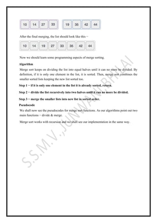
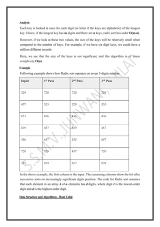
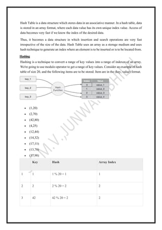
The document discusses various sorting techniques used in computer science. It describes insertion sort, selection sort, and merge sort. Insertion sort maintains a sorted sub-list and inserts new elements into the correct position within the sub-list. Selection sort divides the list into sorted and unsorted parts, selecting the minimum element from unsorted each time. Merge sort divides the list into halves recursively until single elements remain, then merges the halves back together in sorted order.


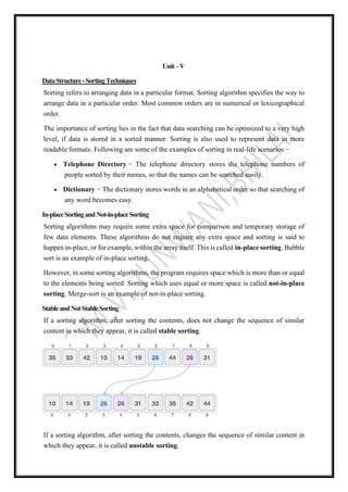
![Algorithm
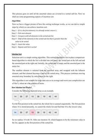
Step 1 − Set MIN to location 0
Step 2 − Search the minimum element in the list
Step 3 − Swap with value at location MIN
Step 4 − Increment MIN to point to next element
Step 5 − Repeat until list is sorted
Pseudocode
procedure selection sort
1. list : array of items
2. n : size of list
3. for i = 1 to n - 1
4. /* set current element as minimum*/
5. min = i
6. /* check the element to be minimum */
7. for j = i+1 to n
8. if list[j] < list[min] then
9. min = j;
10. end if
11. end for
12. /* swap the minimum element with the current element*/
13. if indexMin != i then
14. swap list[min] and list[i]
15. end if
16. end for
17. end procedure](https://image.slidesharecdn.com/unit-vdatastructure-converted-201128113221/85/Unit-v-data-structure-converted-9-320.jpg)
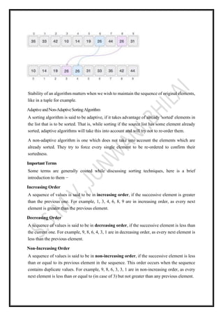
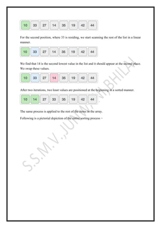
![procedure mergesort( var a as array )
if ( n == 1 ) return a
var l1 as array = a[0] ... a[n/2]
var l2 as array = a[n/2+1] ... a[n]
l1 = mergesort( l1 )
l2 = mergesort( l2 )
return merge( l1, l2 )
end procedure
procedure merge( var a as array, var b as array )
var c as array
while ( a and b have elements )
if ( a[0] > b[0] )
add b[0] to the end of c
remove b[0] from b
else
add a[0] to the end of c
remove a[0] from a
end if
end while
while ( a has elements )
add a[0] to the end of c](https://image.slidesharecdn.com/unit-vdatastructure-converted-201128113221/85/Unit-v-data-structure-converted-12-320.jpg)
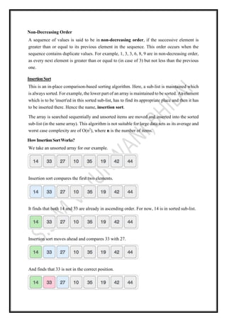
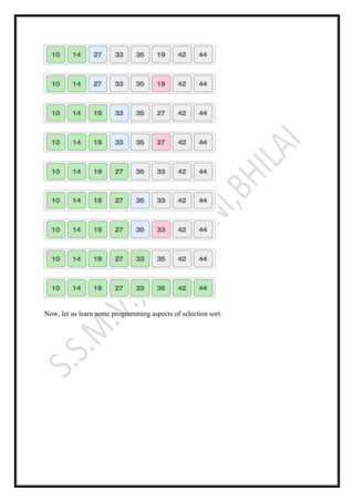
![remove a[0] from a
end while
while ( b has elements )
add b[0] to the end of c
remove b[0] from b
end while
return c
end procedure
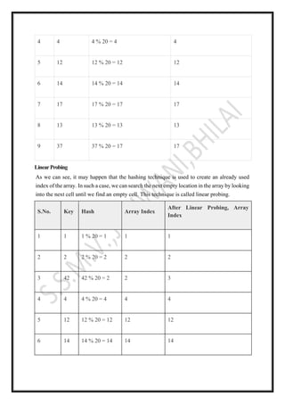
RadixSort
Radix sort is a small method that many people intuitively use when alphabetizing a large list
of names. Specifically, the list of names is first sorted according to the first letter of each
name, that is, the names are arranged in 26 classes.
Intuitively, one might want to sort numbers on their most significant digit. However, Radix
sort works counter-intuitively by sorting on the least significant digits first. On the first pass,
all the numbers are sorted on the least significant digit and combined in an array. Then on the
second pass, the entire numbers are sorted again on the second least significant digits and
combined in an array and so on.
Algorithm: Radix-Sort (list, n)
shift = 1
for loop = 1 to keysize do
for entry = 1 to n do
bucketnumber = (list[entry].key / shift) mod 10
append (bucket[bucketnumber], list[entry])
list = combinebuckets()
shift = shift * 10](https://image.slidesharecdn.com/unit-vdatastructure-converted-201128113221/85/Unit-v-data-structure-converted-13-320.jpg)
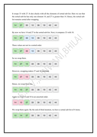
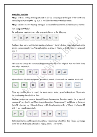
![Example
struct DataItem *search(int key) {
//get the hash
int hashIndex = hashCode(key);
//move in array until an empty
while(hashArray[hashIndex] != NULL) {
if(hashArray[hashIndex]->key == key)
return hashArray[hashIndex];
//go to next cell
++hashIndex;
//wrap around the table
hashIndex %= SIZE;
}
return NULL;
}
InsertOperation
Whenever an element is to be inserted, compute the hash code of the key passed and locate
the index using that hash code as an index in the array. Use linear probing for empty location,
if an element is found at the computed hash code.](https://image.slidesharecdn.com/unit-vdatastructure-converted-201128113221/85/Unit-v-data-structure-converted-18-320.jpg)
![Example
void insert(int key,int data) {
struct DataItem *item = (struct DataItem*) malloc(sizeof(struct DataItem));
item->data = data;
item->key = key;
//get the hash
int hashIndex = hashCode(key);
//move in array until an empty or deleted cell
while(hashArray[hashIndex] != NULL && hashArray[hashIndex]->key != -1) {
//go to next cell
++hashIndex;
//wrap around the table
hashIndex %= SIZE;
}
hashArray[hashIndex] = item;
}
DeleteOperation
Whenever an element is to be deleted, compute the hash code of the key passed and locate the
index using that hash code as an index in the array. Use linear probing to get the element ahead
if an element is not found at the computed hash code. When found, store a dummy item there
to keep the performance of the hash table intact.](https://image.slidesharecdn.com/unit-vdatastructure-converted-201128113221/85/Unit-v-data-structure-converted-19-320.jpg)
![Example
struct DataItem* delete(struct DataItem* item) {
int key = item->key;
//get the hash
int hashIndex = hashCode(key);
//move in array until an empty
while(hashArray[hashIndex] !=NULL) {
if(hashArray[hashIndex]->key == key) {
struct DataItem* temp = hashArray[hashIndex];
//assign a dummy item at deleted position
hashArray[hashIndex] = dummyItem;
return temp;
}
//go to next cell
++hashIndex;
//wrap around the table
hashIndex %= SIZE;
}
return NULL;
}](https://image.slidesharecdn.com/unit-vdatastructure-converted-201128113221/85/Unit-v-data-structure-converted-20-320.jpg)