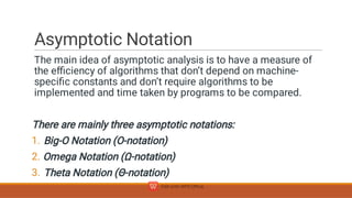
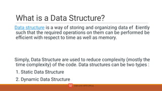
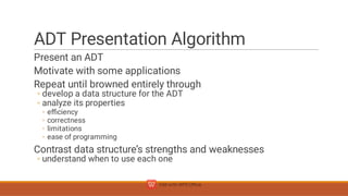
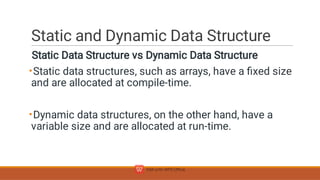
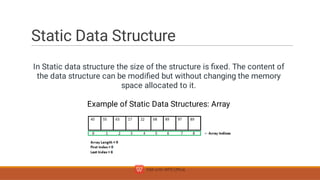
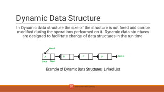
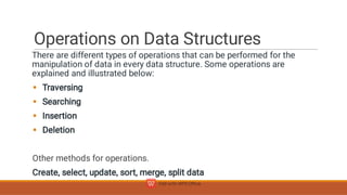
The document provides an introduction to data structures. It defines a data structure as a way of storing and organizing data efficiently to allow operations to be performed quickly. Data structures can be static or dynamic. An abstract data type (ADT) is a mathematical description of an object and its operations. Algorithms implement ADTs using data structures. There are many data structures because there are tradeoffs between speed, memory usage, elegance, and other factors. Common data structures include lists, trees, hash tables. Operations on data structures include traversing, searching, insertion, deletion and others. Static structures have fixed sizes while dynamic structures have variable sizes.

![Traversing Data Structure
Traversing a Data Structure means to visit the element stored in it. It
visits data in a systematic manner. This can be done with any type of DS.
int main()
{
// Initialise array
int arr[] = { 1, 2, 3, 4 };
// size of array
int N = sizeof(arr) / sizeof(arr[0]);
// Traverse the element of arr[]
for (int i = 0; i N; i++) {
// Print the element
cout arr[i] ' ';
}
return 0;
}](https://image.slidesharecdn.com/uniti-240413015826-fd885ced/85/Unit-1-Introduction-to-Data-Structuresres-13-320.jpg)
![Searching Data Structure
Searching means to find a particular element in the given data-structure.
It is considered as successful when the required element is found.
Searching is the operation which we can performed on data-structures
like array, linked-list, tree, graph, etc.
for (int i = 0; i N; i++) {
// If Element is present then
// print the index and return
if (arr[i] == K) {
cout Element found!;
return;
}
}
cout Element Not found!;
}](https://image.slidesharecdn.com/uniti-240413015826-fd885ced/85/Unit-1-Introduction-to-Data-Structuresres-14-320.jpg)
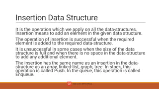
![Insertion Data Structure
int main()
{
// Initialise array
int arr[4];
// size of array
int N = 4;
// Insert elements in array
for (int i = 1; i 5; i++) {
arr[i - 1] = i;
}
// Print array element
printArray(arr, N);
return 0;
}](https://image.slidesharecdn.com/uniti-240413015826-fd885ced/85/Unit-1-Introduction-to-Data-Structuresres-16-320.jpg)