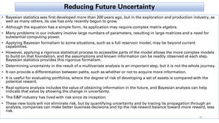
This document discusses understanding and quantifying uncertainty when evaluating projects. It describes how incorporating probabilistic risk analysis and decision analysis can help indicate where more information is needed to reduce uncertainty and risk. Three case studies are presented that use uncertainty analysis for geosteering into a thin reservoir, interpreting well logs in shaly sands, and analyzing a walkaway vertical seismic profile. Quantifying uncertainty allows assessing the value of obtaining additional data.

1. UNDERSTANDING UNCERTAINTY
1

2. Understanding Uncertainty
What is the value of obtaining additional information for any project you plan?
How likely is the project to succeed with or without the new data?
This article describes a way to assess how new information decreases uncertainty and project risk.
Incorporating the method into real-time evaluation programs allows continual updating of prognoses, such as
the distance to a drilling target.
Ian Bryant
Alberto Malinverno Michael Prange
Ridgefield, Connecticut, USA
Mauro Gonfalini
Eni Agip Milan, Italy
James Moffat
Moscow, Russia
Dennis Swager
Team Energy, LLC Bridgeport, Illinois, USA
Philippe Theys
Sugar Land, Texas, USA
Francesca Verga
Politecnico di Torino Turin, Italy
2
Oilfield Review Autumn 2002

3. • Risk is good.
• Risk is bad.
• Companies are driven by a profit motive and in a competitive business climate, making a profit is usually
impossible without some exposure to risk.
• What is the boundary of acceptable risk?
• Accurately judging when risk becomes recklessness is imperative.
• Finding ways to reduce exposure to risk is a difficult but essential business practice; quantifying risk and assessing
the value of information designed to reduce risk can be even more problematic.
• Finding and developing oil and gas assets has always been a risky business.
• The industry has a history of technological advances that diminished risk, even as reservoirs and the way they are
produced have grown in complexity.
• An early development, the use of wireline logging in an oil well by Conrad and Marcel Schlumberger, had its 75th
anniversary September 5, 2002.
• Over the past decade, three-dimensional (3D) seismic surveys have significantly reduced uncertainty about
structures, identified bypassed zones and improved project economics.
• Economic evaluation also has improved.
• Simple deterministic modeling outputs a single value that may be augmented with a few sensitivity cases.
• Slightly more sophisticated evaluation uses ranges of values and can determine which parameters have the
greatest impact on a result.
• The next improvement assigns probability density functions to the ranges of parameters and results in an
expectation curve of economic parameters, such as net present value (NPV) or reserves produced. 3

4. • A fully integrated, multidisciplinary, probabilistic approach, known as decision and risk analysis,
incorporates many more base parameters and propagates uncertainty.
• A study of operators on the Norwegian continental shelf indicated that corporate financial performance
improved after companies integrated decision and risk analysis into their workflows.
• Sophisticated risk analysis can indicate which unknown factors have the greatest impact on project
economics, and technology may exist to obtain that information, but a question remains:
o is the value of additional information worth the cost to obtain it?
• To answer the question for any specific case, a company first must evaluate the degree of project
uncertainty with and without the new information.
• In this article, we investigate sources of uncertainty and a method to propagate uncertainty throughout a
project analysis.
• Propagating uncertainty allows the impact of adding information about an input parameter to carry through
to the result.
• A probabilistic model that explicitly includes probability distributions for parameters can indicate the degree
of uncertainty reduction to be expected by obtaining more information.
• Three case studies show uncertainty analysis for geosteering into a thin pay section, a shaly-sand
petrophysical analysis and a walkaway vertical seismic profile (VSP).
4

5. The Probability of Error
• A fundamental driver for risk analysis is the amount of uncertainty remaining when a decision must be
made.
• If all information were known precisely, there would be no risk in making decisions; the outcome could be
predicted with certainty.
• The quality of measurements available to the exploration and production (E&P) industry is high, but logging
samples a small volume of the reservoir, and coring wells returns an even smaller fraction of the reservoir
for study.
• Although a 3D seismic survey samples the entire reservoir, the vertical resolution is low.
• Fundamental limitations imposed by physics and geometry restrict the amount and quality of information
available.
• Reservoir information is interpreted through models, which are rarely exact for every possible case (see
“Cataloging Errors” Slides 45-48).
• There is one true value that describes a physical quantity at a specific point in space and time.
• For example, the strength of a given block of cement under a given set of conditions has a single value.
• Errors involved in measuring prevent exact determination of that value and require a distribution of possible
answers to represent uncertainty.
• Analysis has to rely on these probability distributions.
• The term “probability” has two common meanings.
• One sense relates to a relative frequency of an event in repeat trials, such as flipping a coin many times.
• If the coin is balanced and fair, and the coin-flipping process also is fair, then about half of the results will be
“heads.”
• The more times the coin is flipped, the closer the outcome will be to 50% (Fig 1). 5

6. Fig 1 Frequency of heads from a fair coin toss.
After one coin toss, either zero or one result will be heads, with the two results having equal probability (dot size
indicates probability).
The most likely result of two tosses is that half the results are heads.
After three tosses, either one or two heads is most likely, giving fractional results of 1⁄3 or 2⁄3.
The probability of obtaining all heads or all tails decreases with each additional toss.
A one-sigma standard deviation (curves) from the mean of the result indicates the most likely fractional number of
heads approaches 0.5 as the number of coin flips increases. 6

7. • The other use of the word relates to a belief or degree of confidence in an uncertain proposition.
• For example, flip a coin but do not look at how it lands.
• The result is already determined; either it is heads or it is “tails.”
• Yet, we still talk about the probability of getting heads as being 50% because that is the degree of belief in
that outcome.
• Both meanings are used in the E&P industry.
• Well-logging tools that rely on radioactive processes either sample at one station for a period of time or log
at a slow speed to increase the counting statistics.
• Counting involves the relative frequency of an event, the first sense of probability.
• An example of probability as belief is the common use of probabilities P10, P50 and P90 to describe the
range of NPV results from a large number of reservoir-economics evaluations obtained by varying input
parameters with each trial.
• The NPV of an actual reservoir under the development conditions modeled is a set, but unknown, value.
• Probabilities expressed as degrees of belief always depend on the available information.
• Based on what is known about the reservoir, that NPV has a 10% probability of being at the P10 model
result or less, an equal chance of being greater or less than the P50 median and a 90% probability of being a
value less than or equal to the P90 prediction.
• A proper analysis of data follows a logical process, meaning we start with premises and create logical
arguments to lead to conclusions.
• Both the premises and the conclusions are statements, or propositions, that can be either true or false.
7

8. • Deductive logic takes the classic form of:
o Premise 1:If A is true, then B is true.
o Premise 2: A is true.
o Conclusion:Therefore, B is true.
• As an example, substitute the statement that the water cut of this well exceeds 99% for A, and substitute the
statement that this well is not economic for B.
• The statements become:
o Premise 1: If the water cut of this well exceeds 99%, then this well is not economic.
o Premise 2:The water cut of this well exceeds 99%.
o Conclusion:Therefore, this well is not economic
• However, just because an argument is cast into a logical form, it may not be valid.
• Even this simple argument can be wrong if the premises are false-the water cut may not exceed 99% after
all.
• Logical arguments usually are not as straightforward as this, and if the conclusions do not derive from the
premises, the argument also can be wrong.
• Arguments involving uncertain propositions fall into a branch called inductive logic, which uses probability
rather than certainty in the argument.
• Some of the probabilities to be used are termed conditional probabilities: the probability of one event being
true when another is known to be true.
• For example, in a given area, there may be an equal probability of a rock encountered at a given depth being
either sandstone or limestone. 8

9. • However, given a log indicating that the formation has a density of 2.3 g/cm3, the probability is very high
that it is a sandstone formation.
• Including probability statements in a generalized inductive argument gives:
o Premise 1: If B is true, then the probability that A is true is P(A|B).
o Premise 2: The probability that A is true is P(A).
o Premise 3:The probability that B is true is P(B).
o Conclusion: There is a probability P(B|A) that B is true given A is true.
• Premise 3 may seem odd, since the objective is to reach a conclusion about B.
• The third premise is a statement about the probability of B occurring in general, while the conclusion is a
conditional statement about B given that A is true.
• The importance of this distinction becomes more apparent using a specific case.
• Suppose a person is tested for a rare virus.
• The test is not always correct.
• In 5% of the cases, the test is positive when the person is not infected, termed a false positive.
• False negatives—the test result is negative when the person is infected-occur in 10% of the cases.
• Represent the statement that the person is infected as Infected, and represent the statement that the test is
positive by Yes.
• The test result on a specific person is positive: according to the test that person is infected.
9

10. • How likely is it that the person actually has the virus?
• The answer is not 90%; that is P(Yes|Infected), the probability the result is positive if the person is infected.
• Nor is the answer 5%; that is the probability the test is positive if the person is not infected, P(Yes|not
Infected).
• The result desired is P(Infected|Yes), the probability that the person is infected when the test is positive.
• That answer relies critically on how rare the virus is in the general population, P(Infected).
• In this case, assume that rare means 10 people are infected for each 1,000,000 of the population not infected,
about 0.001%.
• Testing a random selection of 1,000,010 people results in 50,000 uninfected people obtaining a positive
result, since the test gives 5% false positives, and nine true positives.
• The probability that a person is infected if the test is positive is 0.018%-much higher than the rate in the
general population.
• The test is not definitive because the infection is rare, so false positives still greatly outnumber true positives.
• A positive test result suggests a second, independent test should be performed.
10

11. Bayes’ Rule
• Conditional results like the preceding example can be calculated using Bayes’ rule for propositions.
• Bayes’ rule provides a way to calculate one conditional probability, P(B|A), when the opposite conditional
probability, P(A|B), is known (Fig 2).
• For that reason, it is also known as the rule of inverse probability.
• Bayesian statistics starts with general information about the probability of B, P(B), which is called the prior
probability because it describes what is known before the new information is obtained.
• The likelihood, P(A|B), contains new information specific to the instance at hand.
• From the prior and the likelihood distributions, Bayes’ rule results in the conditional probability of B when A
has occurred, P(B|A), called the posterior probability.
• The denominator is a normalizing factor that involves only A—the total probability of A occurring.
• A simple example demonstrates the use of Bayesian formalism.
• A company has to decide whether to develop a small reservoir in a basin where 14% of small reservoirs like
it have already proven to be productive and economic.
• Interpretation of this particular reservoir, based on a seismic study and well logs, indicates the hydrocarbon
accumulation is economic.
• From past experience, interpretation of this type of data correctly predicts an economic reservoir 80% of the
time, and correctly predicts an uneconomic reservoir 75% of the time.
• Is this reservoir likely to be economic?
11

12. Fig 2 Bayes’ rule for propositions.
12

13. • The prior information, P(Economic), is that 14% of this type of field in this area is economic.
• The new information is a test result of Yes, that is, the analysis indicates this particular reservoir is economic.
• This enters in the likelihood, P(Yes|Economic).
• P(Yes), which appears in the denominator of Bayes’ rule, is not given but it can be calculated.
• The probability can be split into two parts, the probability that the analysis result is Yes and the reservoir is
Economic and the probability that the analysis says Yes but the reservoir is Uneconomic.
• These two conditions do not overlap and they include all conditions, so dividing the probability of Yes into these
two pieces does not affect the total probability.
• The combined probability, for example of Yes and Economic, can be obtained from the conditional probability of
Yes, given that the reservoir is Economic, times the probability the reservoir is Economic.
• Thus, the unknown P(Yes) can be determined from known quantities.
• The result is somewhat surprising.
• Even though the analysis is reasonably accurate, with an 80% rate of successfully predicting economic reservoirs,
the chance this reservoir is economic is 34% (Fig 3).
• The posterior result is driven down to a low level by the prior—the low probability of the general population of
this type of field being economic.
• Intuition can be wrong, particularly when the probability of an outcome given a known test result, such as
P(Economic|Yes), is confused with P(Yes|Economic), the probability of a test result given a known outcome.
• Nonetheless, the value of the additional information provided by the analysis is clearly demonstrated by the
increase in the probability of economic success from 14% to 34%.
• Probabilistic reasoning logically propagates uncertainty from premises to a conclusion. 13

14. Fig 3 Bayes’ rule for a synthetic reservoir case.
A test involving log and seismic interpretation (upper left) provides a test of the economics of a prospect.
It correctly identifies economic prospects 80% of the time and uneconomic prospects 75% of the time.
In this area, 14% of similar fields are economic (upper right).
The numerator in Bayes’ rule can be calculated by splitting the probability that the test gives a Yes indication
into the condition that the Yes indication is correct and the condition that the Yes indication is incorrect
(middle right).
Each of those terms can be defined by a mathematical relation of the probabilities of two independent
quantities taken together (middle left).
When the given values are substituted into Bayes’ rule, the result is only a 34% probability that the new
reservoir is economic, even though the test indicates it is economic (bottom). 14

15. • However, even proper use of the probabilistic formalism does not guarantee the result is correct.
• The conclusion is only as good as the premises and assumptions made at the outset.
• The advantage of using a logically sound method like Bayesian formalism is that incorrect conclusions indicate
some premises or assumptions are unsound—a feedback loop in the interpretation process.
• Another term is sometimes explicitly included in each term of Bayes’ rule representing the general knowledge and
assumptions that go into the evaluation of probability.
• In the reservoir example, the likelihood term, P(Yes|Economic), may assume that the latest generation of logging
tools was used and that the seismic section was interpreted assuming layered formations.
• The prior, P(Economic), may assume that all of the reservoirs are fluvial.
• All of these assumptions are summarized as additional information I, so the likelihood becomes P(Yes|Economic, I)
and the prior becomes P(Economic, I).
• Explicitly incorporating known assumptions and information, I, about the problem into the Bayesian formalism is a
way of indicating the conditions under which the probabilities were calculated.
• The choice of information included in a scenario reflects analyst bias.
• Transparency about all assumptions in the process makes an effective feedback loop possible.
• The probabilities of the prior and likelihood are not always known precisely. Each parameter involved may have an
uncertainty associated with it (Fig 4).
• The simple algebra of Bayes’ rule must be converted to matrix algebra, and if there are a large number of uncertain
parameters, a high-speed computer may be needed to determine the posterior distribution from the prior
distribution and the likelihood.
15

16. Fig 4 Bayes’ rule constraining layer thickness.
Thickness of layers in a reservoir model may be uncertain.
Prior information for layer thickness h for layers. i and j may be poorly constrained, as indicated by the circle on
the crossplot of layer thickness (left).
Darker areas correspond to higher values of the probability distributions, and the dashed lines show bounding
values for the uncertainty.
Log data providing likelihood information indicating one layer gets thinner as the other gets thicker also have
some uncertainty (middle).
The product of these two gives the posterior distribution and properly accounts for all information (right). 16

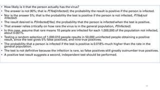
17. Geosteering Through Uncertainty
• Team Energy, LLC, operator of the East Mount Vernon unit, drilled the Simpson No. 22 well, the first
horizontal well in the Lamott Consolidated field in Posey County, Indiana, USA (Fig 5).
• Schlumberger wished to test novel completion technologies to drain oil from a 13-ft [4-m] thick oil column in
this unit.
• The project allowed Schlumberger to test Bayesian uncertainty methods that were incorporated into a
software collaboration package.
• This process successfully helped to locate and steer a horizontal well in a thin oil column.
• The East Mount Vernon unit is highly developed with vertical wells drilled on 10-acre [40,500 m2] spacing;
most wells are openhole completions exposing only the upper 2 to 5 ft [0.6 to 1.5 m] of the oil column.
• The majority of cumulative production is from the Mississippian Cypress sandstone reservoir, although
production also comes from the shallower, MississippianTar Springs reservoir.
• The existing vertical wells produce at a very high water cut, about 95%, because the Cypress reservoir oil
column is so thin.
• The Simpson No. 22 well was drilled first as a deviated pilot well, to penetrate the Cypress sandstone close to
the planned heel of the horizontal section, and subsequently drilled along a smoothly curving trajectory
leading into a horizontal section in the reservoir.
• Geosteering a wellbore is intrinsically a 3D problem.
• Trying to model the process in two dimensions can lead to inconsistent treatment of data from other wells.
• Schlumberger built a 3D earth model that contains the significant stratigraphic features of the Cypress
reservoir.
17

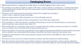
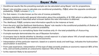
18. Fig 5 Location of the Mount Vernon unit of the Lamott
Consolidated field, near Evansville, Indiana, USA.
The outlined area indicates the modeled area for the
Simpson 22 horizontal well.
Eight offset wells (labeled) were used to constrain the
model around the build section (black) and the 808-ft [246-
m] horizontal section (red) of the well.
18

19. • The model had 72 layers on a grid with five cells on a side. Gamma ray and resistivity values were assigned
to each cell in the model based on well-log data.
• The parameters defining the geometry of the earth model, the thickness of each layer at each grid point, were
represented in the model as a probability distribution.
• Information from the field based on well logs defined the mean of each layer thickness. Combining all these
values defined the mean vector of the model.
• Layer- thickness uncertainty and the interrelation between the uncertainties in thickness at different locations
define the model covariance matrix.
• The mean vector and the covariance matrix together define the model probability distribution.
• A log-normal distribution of thickness prevents layer thickness from becoming negative and describes the
population of thickness values better than a normal distribution.
• The initial model was constrained using horizons picked off logs from eight offset wells.
• The initialization procedure accounted for uncertainty in the measured depth of the horizon pick and
uncertainty in the well trajectory.
• This prior distribution in the 3D earth model was the starting point for drilling the pilot well.
• Even after the information obtained from offset wells was included, the uncertainty in locating the depth to
the top of the 13-ft target zone was about 10 ft [3 m], a significant risk for such a narrow target.
• Scientists at the Schlumberger-Doll Research Center in Ridgefield, Connecticut, USA, created a user interface
to update the 3D earth model quickly and easily across a secure, global computer network.
• In collaboration with drillers at the rig in Indiana, log-interpretation experts in Ridgefield updated the model
while drilling.
• Later in the drilling process, other interpreters were able to monitor the drilling of the horizontal section from
England and Russia in real time by accessing the Schlumberger network.
19

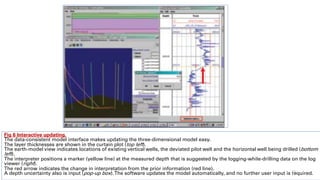
20. • Interpretation experts compared real-time logging-while-drilling (LWD) measurements of gamma ray and
resistivity with a 3D earth model that included uncertainty.
• Using the software, an interpreter could pick a new horizon location and assign an uncertainty to that
location (Fig6).
• The update procedure automatically combined this new information with the prior distribution.
• Use of the Bayesian statistical procedure ensured that the previous picks and all offset-well information were
still properly accounted for and the interpretation was properly constrained (Fig 7).
• The new model from the posterior distribution was immediately available through a secure Web interface so
drillers at the rig could update the drilling plan.
• The procedure was repeated each time the drill bit passed another horizon.
• The posterior distribution from the application of data from one horizon became the prior distribution for the
next horizon. Uncertainty for horizons yet to be reached was reduced with each iteration, decreasing the
project risk.
• The pilot well provided information to update the model near the proposed heel of the horizontal well.
• The logs established that a high-permeability layer, close to the middle of the original oil column, had been
flooded with reinjected produced water.
• This narrowed the window for the horizontal section to the upper half of the reservoir interval.
• The build section of the new well was drilled at 4o per 100 ft [30 m] to enter the formation close to
horizontal.
• The 3D earth model was again updated as the well was drilled, and the wellbore successfully entered the
target formation at 89o. 20

21. Fig 6 Interactive updating.
The data-consistent model interface makes updating the three-dimensional model easy.
The layer thicknesses are shown in the curtain plot (top left).
The earth-model view indicates locations of existing vertical wells, the deviated pilot well and the horizontal well being drilled (bottom
left).
The interpreter positions a marker (yellow line) at the measured depth that is suggested by the logging-while-drilling data on the log
viewer (right).
The red arrow indicates the change in interpretation from the prior information (red line).
A depth uncertainty also is input (pop-up box).The software updates the model automatically, and no further user input is required.
21

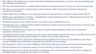
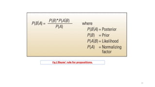
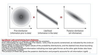
22. Fig 7 Depth uncertainty before and after updating.
Before updating (upper left), the curtain plot indicates the uncertainty in depth of the Cypress is about
8 feet [2.4 m] (orange band).
After the 3D model is updated (lower left), the intersection of the well trajectory with the top of the Cypress
formation in the model is at a measured depth (MD) of 3020 ft [920 m] (red line), and the depth uncertainty is
significantly smaller than before.
The vertical axes of the curtain plots (upper and lower left) are true vertical depth.
22

23. • The next problem was how to keep the well path within a narrow pay interval.
• LWD resistivity logs transmitted to surface in real time were critical to staying within the pay. (Fig 8).
• Schlumberger is the only company that can record images while drilling and transmit them to surface in real
time, using mud-pulse telemetry.
• Patterns in the RAB Resistivity-at-the- Bit image clearly showed how well the trajectory stayed parallel to
formation bedding. Using the 3D earth model updated in real time, drillers kept the 808-ft [246-m] drainhole
within a 6-ft [1.8-m] oil-bearing layer.
• The well was instrumented downhole with pressure sensors and valves that can be opened or closed in real
time.9
• Valves in three separate zones can be set to any position between fully opened and fully closed.
• These valves allowed Schlumberger andTeam Energy, LLC, to test a variety of operating conditions.
• Currently, com- mingling production from two lower zones delivers the best output of oil.
• The 30% water cut is significantly better than the 95% water cut of conventional wells in the field.
• Although not used on the Simpson No. 22 Well, a similar analysis is available in the Bit On Seismic software
package.
• With SeismicVISION information obtained during the drilling process, the location of markers can be
determined while drilling.
• Through Bayesian statistics, the uncertainty in the location of future drilling markers can be evaluated, and
the drilling-target window tightened.10
23

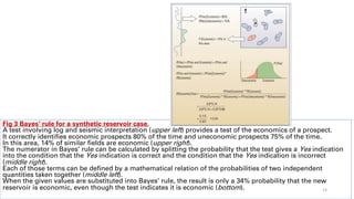
24. Fig 8 Logging-while-drilling (LWD) logs in a 20-ft [6-m] horizontal section.
LWD resistivity images transmit- ted to surface in real time show the well going downdip (left) and parallel to the
geological layering (middle).
More detailed images are downloaded from the tool after drilling (right), showing the same section as in the middle
illustration.
Interpreted stratigraphic dips (green) and fractures (purple) are indicated.
The straight lines are orientation indicators. 24

25. Determining Formation Uncertainty
• The geosteering problem used a model with multivariate normal, or Gaussian, distributions that can be
solved analytically.
• If the variable distributions cannot be assumed to have a simple, Gaussian shape, or when errors are not
small, a Monte Carlo approach is more appropriate.
• In this method, the probability distribution function can have an arbitrary form, but the procedure requires
more computing power than does an analytical approach.
• In a Monte Carlo simulation, values for the parameters are randomly selected from the possible
population, and the scenario is solved. Iterating a random selection followed by model inversion a large
number of times results in a distribution of scenario outcomes.
• In collaboration with researchers at the university Politecnico di Torino, Italy, Eni Agip evaluated
uncertainty in shale volume, porosity and water saturation for several shaly-sand forma- tions.
• The study compared the computationally easy analytic approach, which assumes normal distributions,
with the more complex Monte Carlo method.
• The formations studied had similar lithologies, but each formation had different electrical properties,
porosity ranges and shale content.
• Uncertainty was applied only to log measurements, including resistivity, neutron, density, gamma ray,
sonic and the EPT Electromagnetic Propagation Tool logs. Instrument error was used to define one
standard deviation in the uncertainty distribution (Fig 9).
• When the shale content was negligible, the analysis used Archie’s model to determine water saturation,
Sw. 25

26. 26
Fig 9 Instrument error.
Standard deviation for density is constant; all the others are a percentage of the measured value.

27. • The analysis did not factor in uncertainty related to core-based measurements of a, m and n. Including error in
these core-based measurements can be done, but for simplicity it was omitted in this study.
• There is a hyperbolic relationship between Sw and porosity, which skews the uncertainty distribution in the
analysis (Fig 10).
• A normal distribution of porosity error results in a log-normal distribution of Sw error.
• Since Sw cannot exceed 100%, near that limit the distribution is distorted even more.
• The two error-analysis procedures give simi- lar uncertainty bands for total porosity and effective porosity, except
at low values of porosity where the error distributions are affected by
• restrictions on the values of porosity, shale and matrix volumes to be between zero and one.
• Today, the best procedure for determining shale content uses spectroscopy data from tools such as the ECS
Elemental Capture Spectroscopy sonde.
• The data are transformed from elemental concentration to clay content using SpectroLith lithology processing.
• However, such data were not available for these wells. Several shale- volume, Vshale, indicators have been used
by the industry, including two based on logs run on these wells.
• Both the gamma ray and the EPT logs give reasonable results for Vshale under ideal conditions, but those
conditions are different for each indicator (Fig 11).
• The common industry practice when using a deterministic approach is to accept the Vshale indicator having the
lowest value at each level.13
• A Monte Carlo simulation provided uncertainty analysis for the shale volume using two indicators, one from the
gamma ray log and one from the EPT attenuation curve (Fig 12).
• Archie’s model was applied to a low-porosity, gas-bearing sandstone formation.
• The analytical- and numerical-uncertainty results differed, particularly for high water-saturation values (Fig13).
• The upper bounds on the error were similar, but the Monte Carlo procedure indicated much tighter lower bounds
on the result than did the analytical procedure.
27

28. Fig 10 Nonlinear relationship between petrophysical parameters affecting probability distributions.
The Archie relationship (formula) for a given formation with constant factors a, m, n and Rt results in a
hyperbolic relationship of water saturation, Sw, to porosity (blue).
This relationship distorts the frequency distributions, which are shown along the axes.
A normal uncertainty distribution about a given porosity value (green) becomes a log-normal distribution
for the resulting Sw uncertainty (red).
The mean value (dashed yellow) and three-sigma points (dashed purple) show the skewed Sw distribution.
Sw distributions determined through Monte Carlo modeling are distorted at high values, since saturation
cannot exceed 100% (inset).
28

29. Fig 11 Determination of shale volume from two indicators.
The gamma ray log (red) and EPT attenuation curve (blue) each provide
an indicator of shale volume.
The minimum of the two indicators was taken as the estimator of Vshale
(shaded purple).
29

30. Fig 12Uncertainty in shale volume.
A Monte Carlo analysis of shale volume used the gamma ray and EPT attenuation (EATT) curves (left).
The uncertainty shows a one-sigma standard deviation (dashed red) around the minimum Vshale (purple).
In a large number of Monte Carlo simulations with uncertainty distributions for the gamma ray and EPT logs,
sometimes the gamma ray log will indicate minimum shale, other times the minimum will come from the EPT
log. Averaging the realizations yields a standard deviation of the result (orange) that falls between the gamma
ray (purple) and the EPT log (red) standard deviations (inset). 30

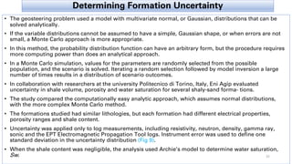
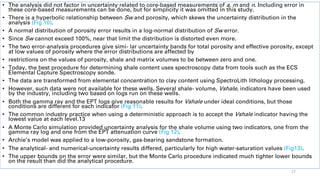
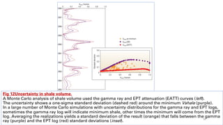
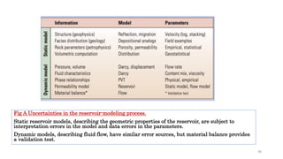
31. Fig 13 Uncertainty in petrophysical measurements.
The input curves for gamma ray, resistivity and density for a low-porosity, gas-bearing formation are shown in the
first three tracks.
An input curve for neutron porosity (green) is compared with porosity derived from the bulk density (blue), which is
shown with one standard deviation error (pink) (Track 4).
Water saturation (blue) was calculated from Archie’s equation using an analytical method (Track 5) and a numerical,
Monte Carlo method (Track 6), with uncertainty bands (pink) indicating a one-sigma standard deviation.
The lower-bound uncertainty near 1209 m [3967 ft] and between 1212 and 1214 m [3977 and 3983 ft] is much larger
u
sing the analytical method than with the numerical, Monte Carlo method. 31

32. • The discrepancy occurred predominantly in the lower-porosity egions (Fig 14).
• The uncertainty associated with water saturation is strongly overestimated by the analytical method—being
as high as 1.6 times the calculated saturation value— whereas uncertainty calculated using the numerical
method is consistently negligible in the low-porosity formations.
• A high-porosity, gas-bearing sandstone formation also showed some discrepancies between the method for
evaluating uncertainty, but only for zones of porosity below 15%. However, the overall good agreement
should be regarded as particular to this case for the following reasons:
• High porosity ranges—in excess of 33%— are rarely found in reservoir rocks.
• Only special combinations of the Archie’s parameters do not amplify error propagated from the porosity log.
• Archie’s formula does not account for errors associated with shale volume, but in formations where shale
fraction is not negligible, the uncertainty associated with shale-volume determination contributes to the
water-saturation uncertainty.
• Water-saturation models more complex than Archie’s equation were used to analyze shaly-sand formations.
• The rock petrophysical properties provided the basis for selecting the most suitable model for each
formation.
• The analyses showed that the form of the mathematical relationship of water saturation to shale volume
impacted the water-saturation uncertainty.14
• Application of the Monte Carlo simulation allowed a more rigorous evaluation of uncertainty and risk
associated with results of a log-interpretation process, because that method is not restricted to a normal
distribution.
• Results from this analysis showed that an appropriate model must be selected and tailored to each for-
mation to obtain a consistent probability distribution of hydrocarbon in place and to perform reliable field
economics .
32

33. Fig 14 Water-saturation relative error at various porosity values in gas-bearing shaly sands.
The relative error, or uncertainty, in water saturation is a smooth function for the analytical results (red), which
overestimate error at low porosity in comparison with the numerical results (purple).
Both a high- porosity formation (upper plot) and a low-porosity formation (lower plot) show a similar trend.
33

34. A Random Walk Toward a Solution
• Monte Carlo methods also have been used in inverse problems.
• The objective of such an analysis is to infer the value of the parameters of a model from a set of measurements, such as obtaining
seismic velocities in the subsurface from a seismic survey.
• A straightforward Monte Carlo methodology, however, is typically time-consuming because only a small proportion of earth
models chosen at random fits the measurements.
• With a large number of parameters, the Markov chain Monte Carlo (MCMC) simulation is more efficient.
• It starts at a random point, or state, in the space of the parameters, and per- turbs the parameters, taking a random walk in
parameter space.
• Each state in parameter space can be assigned an associated figure of merit that measures the quality of that particular choice of
parameters.
• Each step of the random walk is accepted with a probability determined by the Metropolis rule: if the new state is better than the
old state, the step is always accepted; otherwise, the step is accepted with a probability equal to the ratio of the figures of merit of
the new to the old state.
• For example, if the new state is five times worse than the old state, then the step will be taken with a 20% probability.
• This is like a drunkard doing a random walk in a hilly field.
• At each step, the drunkard tests whether a step in a randomly chosen direction will be easy or hard.
• Drunken perception is flawed, so sometimes the uphill step is taken, but, over the long term, the path will tend down- hill.
• Eventually, the random walk will keep wandering near the bottom of the valley.
• Within the Bayesian context, the test involves the posterior probability, which equals the product of the prior probability and the
likelihood function.
• The figure of merit for making a move is the ratio of the posterior probabilities of the proposed state to the current state.
• Since the initial choice is random, the procedure may begin in a highly unlikely state.
• There is a burn-in period, which includes the steps taken as the Metropolis rule moves toward a state of likely parameter values.
• After the burn-in period, the distribution of states approximates the posterior distribution of the parameters.
• Schlumberger used Bayesian analysis with the MCMC-Metropolis algorithm to evaluate a walkaway VSP for a well offshore west
Africa.
34

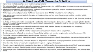
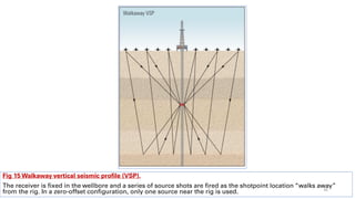
35. • The operator obtained a walkaway VSP because of excess pressure encountered in the well. The walkaway
data extended to a maximum off- set of 2500 m [1.6 miles] from the wellhead (Fig15).
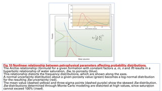
• The data set was used later to investigate uncertainty associated with the prediction of elastic properties
below the bit.
• The model parameters in the earth model are the number and thickness of formation layers, and the
compressional P-wave velocity, the shear S-wave velocity and the formation density for each layer.
• Since these quantities are not known before drilling, determining them from the walkaway VSP data is an
inverse problem, which makes it a candidate for a Bayesian procedure.
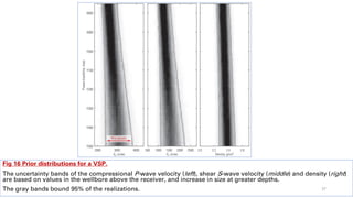
• The prior information incorporates the knowledge of these parameters in the already-drilled portion of the
well (Fig16).
• Uncertainty in the parameters increases with distance away from the known values, that is, from the current
drilled depth.
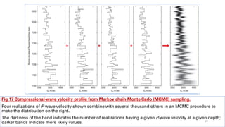
• This prior and the walkaway VSP data were used to develop the probability function in the MCMC procedure.
By superimposing a few thousand earth models that fit the VSP data, the probability distribution of the
parameters can be developed (Fig 17).
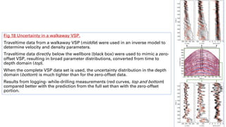
• The first analysis was constrained to seismic reflections near the wellbore.
• This would be the information available from a zero-offset seismic survey (Fig 18).
• The uncertainty band in the predicted elastic properties is fairly broad.
• Including the entire data set makes the uncertainty band much tighter, with long-wavelength velocity
information coming from the variation in walkaway reflection time with offset.
• This improvement in uncertainty represents the increased value of information obtained with a walkaway
VSP compared with a zero-offset VSP.
• This can be combined with an overall project financial analysis to determine the decreased risk based on the
new information. 35

36. Fig 15 Walkaway vertical seismic profile (VSP).
The receiver is fixed in the wellbore and a series of source shots are fired as the shotpoint location “walks away”
from the rig. In a zero-offset configuration, only one source near the rig is used. 36

37. Fig 16 Prior distributions for a VSP.
The uncertainty bands of the compressional P-wave velocity (left), shear S-wave velocity (middle) and density (right)
are based on values in the wellbore above the receiver, and increase in size at greater depths.
The gray bands bound 95% of the realizations. 37

38. Fig 17 Compressional-wave velocity profile from Markov chain Monte Carlo (MCMC) sampling.
Four realizations of P-wave velocity shown combine with several thousand others in an MCMC procedure to
make the distribution on the right.
The darkness of the band indicates the number of realizations having a given P-wave velocity at a given depth;
darker bands indicate more likely values. 38

39. Fig 18 Uncertainty in a walkaway VSP.
Traveltime data from a walkaway VSP (middle) were used in an inverse model to
determine velocity and density parameters.
Traveltime data directly below the wellbore (black box) were used to mimic a zero-
offset VSP, resulting in broad parameter distributions, converted from time to
depth domain (top).
When the complete VSP data set is used, the uncertainty distribution in the depth
domain (bottom) is much tighter than for the zero-offset data.
Results from logging- while-drilling measurements (red curves, top and bottom)
compared better with the prediction from the full set than with the zero-offset
portion.
39

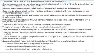
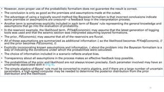
40. Getting the Right Model
• In some cases, the dominant uncertainty may not be in the parameters of a subsurface model, but in
understanding which scenario to apply.
• Available data may not be adequate for differentiating the geologic environment, such as fluvial or tidal
deposition. The presence and number of faults and fractures may be uncertain, and the number of layers in
or above a formation may be unclear.
• The same Bayesian analysis can be applied to choosing the proper scenario as has been applied to
determining probabilities within a given scenario.
• The possible scenarios are designated by a series of hypotheses Hi, where the subscript i designates a
scenario.
• The posterior probability of interest is the probability that a scenario Hi is correct given the data, P(Hi|d).
• The denominator in Bayes’ rule is dependent only on the data, not the scenario, so it is a constant.
• To compare scenarios using Bayes’ rule, compare the product of the prior P(Hi) and the likelihood, P(d|Hi),
the probability of measuring the data d when the scenario Hi is true.
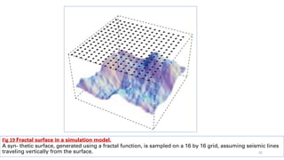
• Bayesian statistics can be applied to scenaios to determine the right size to make a reservoir model based on
seismic data. Modern seismic 3D imaging can resolve features smaller than 10 m [33 ft] by 10 m.
• Reservoir models using such small cells would be huge, generating computational and display problems.
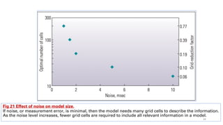
• In addition, even though the data are processed to that level, there is noise in the data.
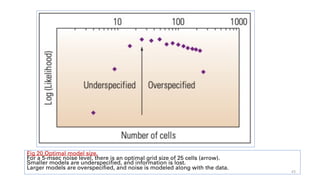
• The optimal model grid size should be larger than the data resolution size so the noise, or error, is not
propagated into the model grid.
• The objective is to obtain a model that contains the optimal degree of complexity, balancing the need to
keep the model small with the need to make the most predictive model possible.
• Statistics allow the information in the data to determine the model size, accounting for measurements, noise
and the desired predictions. 40

41. • To illustrate this, a fractal surface was generated for numerical modeling (Fig19).
• Seismic measurements were simulated using vertical seismic rays from a 16 by 16 regularly sampled grid on
the volume’s surface down to the fractal surface.
• Normally distributed noise with a known standard deviation was added to the measurements.
• Square model grids ranging from 2 to 16 cells on a side were tested using Bayesian statistics to find the
optimal model grid size (Fig 20).
• For a given noise level, models with too few cells do not adequately fit the data; models with too many cells
fit both noise and data.
• In this case, the prior probability P(Hi) will be the same for all scenarios, since no prior information favors
one grid size over another.
• The scenario with the number of grid cells that optimizes the likelihood is the best.
• The optimal number is a function of the amount of noise in the data (Fig 21).
• When a noise level of 5 msec was applied to the data from the fractal surface, the optimal grid had 25 cells.
• This example uses a simple grid, but the Bayesian formulation can be applied to models of arbitrary
complexity.
• This would allow, for example, an optimal refinement of the grid in the vicinity of a well where more detailed
measurements are available.
• An optimal grid used throughout the interpretation workflow delivers several advantages, such as:
o smaller models that do not compromise measurements
o variable local resolution to optimize use of data
o models that intrinsically carry uncertainty information.
41

42. Fig 19 Fractal surface in a simulation model.
A syn- thetic surface, generated using a fractal function, is sampled on a 16 by 16 grid, assuming seismic lines
traveling vertically from the surface. 42

43. Fig 20 Optimal model size.
For a 5-msec noise level, there is an optimal grid size of 25 cells (arrow).
Smaller models are underspecified, and information is lost.
Larger models are overspecified, and noise is modeled along with the data.
43

44. Fig 21 Effect of noise on model size.
If noise, or measurement error, is minimal, then the model needs many grid cells to describe the information.
As the noise level increases, fewer grid cells are required to include all relevant information in a model.
44

45. Reducing Future Uncertainty
• Bayesian statistics was first developed more than 200 years ago, but in the exploration and production industry, as
well as many others, its use has only recently begun to grow.
• Although the equation has a simple form, its application may require complex matrix algebra.
• Many problems in our industry involve large numbers of parameters, resulting in large matrices and a need for
substantial computing power.
• Applying Bayesian formalism to some situations, such as a full reservoir model, may be beyond current
capabilities.
• However, applying a rigorous statistical process to accessible parts of the model allows the more complex models
to build on that foundation, and the assumptions and known information can be readily observed at each step.
Bayesian statistics provides this rigorous formalism.
• Determining uncertainty in the result of a multivariate analysis is an important step, but it is not the whole journey.
• It can provide a differentiation between paths, such as whether or not to acquire more information.
• It is useful for evaluating portfolios, where the degree of risk of developing a set of assets is compared with the
potential reward.
• Real-options analysis includes the value of obtaining information in the future, and Bayesian analysis can help
indicate that value by showing the change in uncertainty.
• The E&P industry has lived with risk since its inception.
• These new tools will not eliminate risk, but by quantifying uncertainty and by tracing its propagation through an
analysis, companies can make better business decisions and tip the risk-reward balance toward more reward, less
risk.
45

46. Cataloging Errors
• Measurement devices, ranging from simple rulers to complex logging sondes, make errors.
• For example, if an object’s length is exactly 5.780 units—such as inches or centimeters— and the ruler being
used is graduated to tenths of a unit, the measurement must be interpolated to determine the digit in the
hundredth’s place.
• Precision can be improved and uncertainty reduced, for example by investing in
a better ruler or improved sonde technology.
• However, improvement will be limited by cur- rent technology and cost.
• Normally, inaccuracy results in larger measurement errors than does imprecision.
• If the quantity is 5.780 and a device is capable of measuring to at least two decimal places, an inaccurate
device would give some number other than 5.78.
• This could be due to a systematic error, such as a warped ruler that always measures too long, or it could be
due to a random error associated with the measurement process.
• Known systematic errors can be accounted for; many logging measurements include environmental corrections,
such as borehole size and borehole-fluid salinity corrections used with resistivity and nuclear tools.
• If repeated measurements of the same quantity using the same device yield different values, the cause is
random errors.
• The causes of such errors are usually beyond our control, and often beyond our understanding.
• Natural variations in the earth cause random variation in measured quantities, such as seismic reflections
from close but not identical wave paths or core analysis results from adjacent and seemingly identical samples.
46

47. • The influence of random errors can be reduced by repeated measurements, or in some cases by spending more
time taking a measurement.
• The user of information from a sophisticated tool often is not interested in the value of a direct measurement.
• The measurement may be a voltage drop or optical density, while the quantity of interest is formation
resistivity or oil gravity.
• Either within the tool software or in post-processing, the measurement is analyzed using a model (Fig A).
• Models are representations of reality—simplifications or generalizations of our understanding of the way the
world works—but they are not reality.
• The Archie equation is not exactly correct, nor are the various modifications to it.
• Petrophysicists try to understand the model’s limitations and the errors associated with using it, but they still
use it for formation evaluation.
• Laboratory and field measurements are subject to quality-control problems, which can be systematic,
equipment or human error.
• A quality-assurance study on density, porosity and air permeability conducted by Amoco, now BP, between 1978
and 1989 involved repeated measurements on stable cores by many laboratories.
• At the beginning of the study, Amoco followed general guidelines for accuracy, but the database grew large
enough to tighten the standards on acceptable error for these measurements.
• The company was able to say with confidence which of the laboratory results were beyond acceptable limits.1
• Human blunders are an important source of error, and they are hard to handle in error analysis.
• Measurement errors of a few percent pale in comparison to the result of transposing the first two digits of a
five-digit number, or losing the only copy of a set of data. 47

48. Fig A Uncertainties in the reservoir-modeling process.
Static reservoir models, describing the geometric properties of the reservoir, are subject to
interpretation errors in the model and data errors in the parameters.
Dynamic models, describing fluid flow, have similar error sources, but material balance provides
a validation test.
48

49. • Data- and information-management systems seek to reduce the chance of human error by designing processes
that do not require data to be input more than one time.
• Real-time data transfers put the information on the computer desktops of users, with minimal human
intervention.
• More subtle human errors also exist. Bias can influence interpretations.
• A strong desire to go forward with a prospect, or conversely to fulfill an obligation and then get out of a
contract, can lead to overly optimistic or pessimistic evaluations of information.
• As another example, financial incentives to drillers to avoid doglegs in a well can lead to the undesired result
of under- reporting of drilling problems.
• These subtle human errors can be difficult to discover.
• The best solution is transparency.
• All steps of a pro- cess need to be traceable, with a catalog of all assumptions made.
• While this might not stop bias from entering the analysis, it can be discovered and corrected at a later time.
49

50. THANK YOU
50