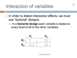
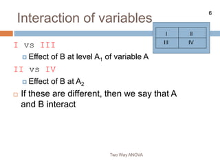
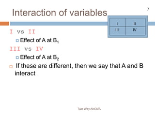
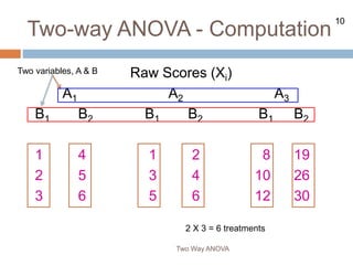
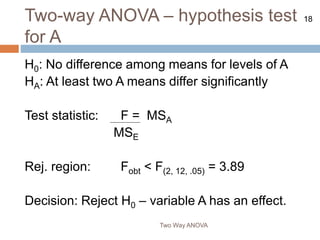
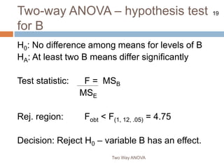
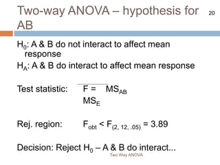
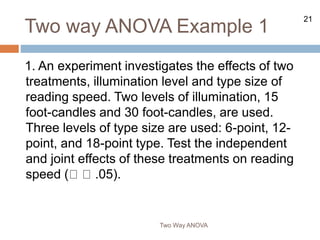
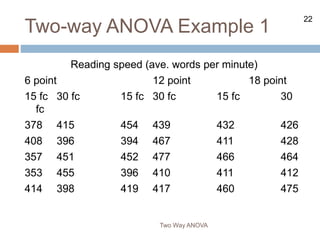
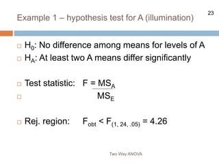
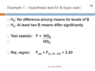
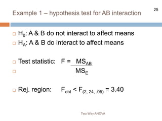
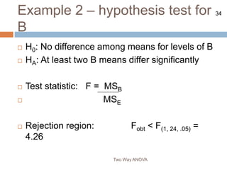
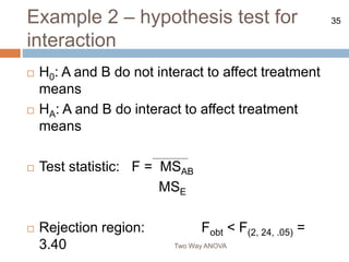
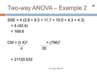
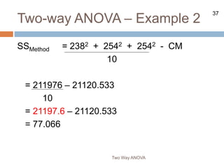
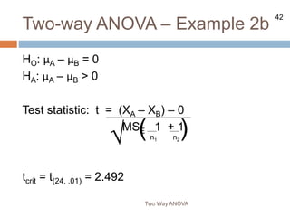
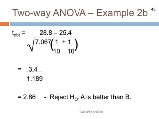
1
The Two-way ANOVA
Two Way ANOVA
 We have learned how to test for the effects of
independent variables considered one at a
time.
 However, much of human behavior is
determined by the influence of several
variables operating at the same time.
 Sometimes these variables combine to
influence performance.
2
The Two-way ANOVA
Two Way ANOVA
 We need to test for the independent and combined
effects of multiple variables on performance. We do this
with an ANOVA that asks:
(i) how different from each other are the means for
levels of Variable A?
(ii) how different from each other are the means for
levels of Variable B?
(iii) how different from each other are the means for the
treatment combinations produced by A and B
together?
3
The Two-way ANOVA
Two Way ANOVA
 The first two of those questions are questions
about main effects of the respective
independent variables.
 The third question is about the interaction
effect, the effect of the two variables
considered simultaneously.
4
The Two-way ANOVA
Two Way ANOVA
 Main effect
 A main effect is the effect on performance of one
treatment variable considered in isolation
(ignoring other variables in the study)
 Interaction
 an interaction effect occurs when the effect of
one variable is different across levels of one or
more other variables
5
Interaction of variables
Two Way ANOVA
 In order to detect interaction effects, we must
use “factorial” designs.
 In a factorial design each variable is tested at
every level of all of the other variables.
A1 A2
B1 I II
B2 III IV
6
Interaction of variables
Two Way ANOVA
I vs III
 Effect of B at level A1 of variable A
II vs IV
 Effect of B at A2
 If these are different, then we say that A
and B interact
I II
III IV
7
Interaction of variables
Two Way ANOVA
I vs II
 Effect of A at B1
III vs IV
 Effect of A at B2
 If these are different, then we say that A and B
interact
I II
III IV
Two Way ANOVA
A1 A2 A1 A2
B1
B2
B1
B2
• In the graphs above, the effect of A varies at levels of
B, and the effect of B varies at levels of A. How you say
it is a matter of preference (and your theory).
• In each case, the interaction is the whole pattern. No
part of the graph shows the interaction. It can only be
seen in the entire pattern (here, all 4 data points).
9
Interaction of variables
Two Way ANOVA
 In order to test the hypothesis about an
interaction, you must use a factorial design.
 The designs shown on the previous slide (2 X 2s)
are the simplest possible factorial designs.
 We frequently use 3 and 4 variable designs, but
beware: it’s very difficult to interpret an interaction
among more than 4 variables!
10
Two-way ANOVA - Computation
Two Way ANOVA
Raw Scores (Xi)
A1 A2 A3
B1 B2 B1 B2 B1 B2
1 4 1 2 8 19
2 5 3 4 10 26
3 6 5 6 12 30
Two variables, A & B
2 X 3 = 6 treatments
Two Way ANOVA
Cell Totals (Tij) and marginal totals (Ti & Tj)
A1 A2 A3 Tj
B1 6 9 30 45
B2 15 12 75 102
Ti 21 21 105 147
Totals for the levels of A are in blue
B Totals
are in red
Cell totals are in green
12
Two-Way ANOVA – Computational
formulas
Two Way ANOVA
CM = (ΣXi)2/N = (147)2 = 1200.5
18
ΣX2 = 12 + 22 + … + 302 = 2427
SSTotal = ΣX2 – CM
SSE = ΣX2 – Σ(Tij)2
nij
Notice that these are the
original data from Slide 10
13
Two-Way ANOVA – Computational
formulas
Two Way ANOVA
Σ(Ti)2/ni = (21)2 + (21)2 + (105)2 = 1984.5
6 6 6
SSA = Σ(Ti)2 – CM
ni
SSA is the sum of squared deviations
for Variable A
14
Two-Way ANOVA – Computational
formulas
Two Way ANOVA
Σ(Tj)2/ni = 452 + 1022 = 1381
9 9
SSB = Σ(Tj)2 – CM
nj
SSB is the sum of squared deviations for
Variable B. It is NOT the sum of squares for
Blocks – this is not a block design!
15
Two-Way ANOVA – Computational
formulas
Two Way ANOVA
Σ(Tij)2/nij = 62 + 152 + … + 302 + 752 = 2337
3 3 3 3
SSAB = Σ(Tij)2 – Σ(Tj)2 – Σ(Ti)2 + (ΣX)2
nij nj ni n
SSAB is the sum of squared deviations for the
interaction of A and B
Two Way ANOVA
We now compute:
SSA = 1984.5 – 1200.5 = 784
SSB = 1381 – 1200.5 = 180.5
SSTotal = 2427 – 1200.5 = 1226.5
SSE = 2427 – 2337 = 90
SSAB = 2337 – 1381 – 1984.5 + 1200.5
= 172
CM
Two Way ANOVA
Source df SS MS F
A a-1 = 2 784 392 52.27
B b-1 = 1 180.5 180.5 24.07
AB (a-1)(b-1) = 2 172 86 11.47
Error n-ab = 12 90 7.5
Total n-1 = 17 1226.5
18
Two-way ANOVA – hypothesis test
for A
Two Way ANOVA
H0: No difference among means for levels of A
HA: At least two A means differ significantly
Test statistic: F = MSA
MSE
Rej. region: Fobt < F(2, 12, .05) = 3.89
Decision: Reject H0 – variable A has an effect.
19
Two-way ANOVA – hypothesis test
for B
Two Way ANOVA
H0: No difference among means for levels of B
HA: At least two B means differ significantly
Test statistic: F = MSB
MSE
Rej. region: Fobt < F(1, 12, .05) = 4.75
Decision: Reject H0 – variable B has an effect.
20
Two-way ANOVA – hypothesis for
AB
Two Way ANOVA
H0: A & B do not interact to affect mean
response
HA: A & B do interact to affect mean response
Test statistic: F = MSAB
MSE
Rej. region: Fobt < F(2, 12, .05) = 3.89
Decision: Reject H0 – A & B do interact...
21
Two way ANOVA Example 1
1. An experiment investigates the effects of two
treatments, illumination level and type size of
reading speed. Two levels of illumination, 15
foot-candles and 30 foot-candles, are used.
Three levels of type size are used: 6-point, 12-
point, and 18-point type. Test the independent
and joint effects of these treatments on reading
speed ( .05).
Two Way ANOVA
22
Two-way ANOVA Example 1
Reading speed (ave. words per minute)
6 point 12 point 18 point
15 fc 30 fc 15 fc 30 fc 15 fc 30
fc
378 415 454 439 432 426
408 396 394 467 411 428
357 451 452 477 466 464
353 455 396 410 411 412
414 398 419 417 460 475
Two Way ANOVA
23
Example 1 – hypothesis test for A (illumination)
Two Way ANOVA
 H0: No difference among means for levels of A
 HA: At least two A means differ significantly
 Test statistic: F = MSA
 MSE
 Rej. region: Fobt < F(1, 24, .05) = 4.26
24
Example 1 – hypothesis test for B (type size)
Two Way ANOVA
 H0: No difference among means for levels of B
 HA: At least two B means differ significantly
 Test statistic: F = MSB
 MSE
 Rej. region: Fobt < F(2, 24, .05) = 3.40
25
Example 1 – hypothesis test for AB interaction
Two Way ANOVA
 H0: A & B do not interact to affect means
 HA: A & B do interact to affect means
 Test statistic: F = MSAB
 MSE
 Rej. region: Fobt < F(2, 24, .05) = 3.40
26
Two-way Anova – Example 1
Two Way ANOVA
Compute:
CM = (12735)2 = 5406007.5
30
SSA = 62052 + 65302 – CM = 3520.833
15
27
Two-way Anova – Example 1
Two Way ANOVA
SSB = 40252 + 43252 + 43852 – CM
10
= 7440.0
Σ(Tij)2 = 19102 + 21152 + … + 21802 + 22052
nij 5 5 5 5
= 5380634.2
28
Two-way Anova – Example 1
Two Way ANOVA
SSAB = 5380634.2 – 5409528.33 – 5413447.5 + 5406007.5
= 1646.667
SSTotal = ΣX2 – CM = 5437581.0 – 5406007.5
= 31573.5
SSE = SSTotal – SSA – SSB – SSAB = 18966.0
29
Two-way Anova – Example 1
Two Way ANOVA
Source df SS MS F
A 1 3520.83 3520.83
4.46*
B 2 7440.00 3720.00
4.71*
AB 2 1646.67 823.33 1.04
Error 24 18966.0 790.25
Total 29 31573.5
* Reject H0.
30
Two-way Anova – Example 2
Two Way ANOVA
 A researcher is interested in comparing the
effectiveness of 3 different methods of
teaching reading, and also in whether the
effectiveness might vary as a function of the
reading ability of the students. Fifteen students
with high reading ability and fifteen students
with low reading ability were divided into three
equal-sized group and each group was taught
by one of these methods. Listed on the next
slide are the reading performance scores for
the various groups at school year-end.
31
Two-way Anova – Example 2
Two Way ANOVA
Teaching Method
Ability A B C
High X 37.6 32.4 33.2
s2 2.8 9.3 11.7
Low X 20.0 18.4 17.6
s2 10.0 4.3 4.3
32
Two-way Anova – Example 2
Two Way ANOVA
 (a) Do the appropriate analysis to answer the
questions posed by the researcher (all αs =
.05)
 (b) The London School Board is currently
using Method B and, prior to this experiment,
had been thinking of changing to Method A
because they believed that A would be better.
At α = .01, determine whether this belief is
supported by these data.
33
Example 2 – hypothesis test for
A
Two Way ANOVA
 H0: No difference among means for levels of A
 HA: At least two A means differ significantly
 Test statistic: F = MSA
 MSE
 Rejection region: Fobt < F(2, 24, .05) =
3.40
34
Example 2 – hypothesis test for
B
Two Way ANOVA
 H0: No difference among means for levels of B
 HA: At least two B means differ significantly
 Test statistic: F = MSB
 MSE
 Rejection region: Fobt < F(1, 24, .05) =
4.26
35
Example 2 – hypothesis test for
interaction
Two Way ANOVA
 H0: A and B do not interact to affect treatment
means
 HA: A and B do interact to affect treatment
means
 Test statistic: F = MSAB
MSE
 Rejection region: Fobt < F(2, 24, .05) =
3.40
36
Two-way ANOVA – Example 2
Two Way ANOVA
SSE = 4 (2.8 + 9.3 + 11.7 + 10.0 + 4.3 + 4.3)
= 4 (42.4)
= 169.6
CM = (Σ X)2 = (796)2
n 30
= 21120.533
37
Two-way ANOVA – Example 2
Two Way ANOVA
SSMethod = 2382 + 2542 + 2542 - CM
10
= 211976 – 21120.533
10
= 21197.6 – 21120.533
= 77.066
38
Two-way ANOVA – Example 2
Two Way ANOVA
SSAbility = 5162 + 2802 - CM
15
= 344656 – 21120.533
15
= 22977.066 – 21120.533
= 1856.533
39
Two-way ANOVA – Example 2
Two Way ANOVA
For the interaction sum of squares, we begin
with the value
ΣT2
ij = 1382 + 1622 + 1662 + …882
nij 5
= 115352
5
= 23070.4
40
Two-way ANOVA – Example 2
Two Way ANOVA
Now, we can compute SSMA:
23070.4 – 21197.6 – 22977.066 + 21120.533
= 16.267
41
Two-way ANOVA – Example 2
Two Way ANOVA
Source df SS MS F
Method 2 77.066 38.533 5.45*
Ability 1 1856.533 1856.533 262.72*
M x A 2 16.267 8.134
1.15
Error 24 169.6 7.067
Total 29
Reject HO for Method and for Ability, not for
interaction.
42
Two-way ANOVA – Example 2b
Two Way ANOVA
HO: μA – μB = 0
HA: μA – μB > 0
Test statistic: t = (XA – XB) – 0
MSE 1 + 1
tcrit = t(24, .01) = 2.492
√ ( )
n1 n2
43
Two-way ANOVA – Example 2b
Two Way ANOVA
tobt = 28.8 – 25.4
7.067 1 + 1
10 10
= 3.4
1.189
= 2.86 - Reject HO. A is better than B.
√ ( )

Twoway.ppt

  • 1.
    1 The Two-way ANOVA TwoWay ANOVA  We have learned how to test for the effects of independent variables considered one at a time.  However, much of human behavior is determined by the influence of several variables operating at the same time.  Sometimes these variables combine to influence performance.
  • 2.
    2 The Two-way ANOVA TwoWay ANOVA  We need to test for the independent and combined effects of multiple variables on performance. We do this with an ANOVA that asks: (i) how different from each other are the means for levels of Variable A? (ii) how different from each other are the means for levels of Variable B? (iii) how different from each other are the means for the treatment combinations produced by A and B together?
  • 3.
    3 The Two-way ANOVA TwoWay ANOVA  The first two of those questions are questions about main effects of the respective independent variables.  The third question is about the interaction effect, the effect of the two variables considered simultaneously.
  • 4.
    4 The Two-way ANOVA TwoWay ANOVA  Main effect  A main effect is the effect on performance of one treatment variable considered in isolation (ignoring other variables in the study)  Interaction  an interaction effect occurs when the effect of one variable is different across levels of one or more other variables
  • 5.
    5 Interaction of variables TwoWay ANOVA  In order to detect interaction effects, we must use “factorial” designs.  In a factorial design each variable is tested at every level of all of the other variables. A1 A2 B1 I II B2 III IV
  • 6.
    6 Interaction of variables TwoWay ANOVA I vs III  Effect of B at level A1 of variable A II vs IV  Effect of B at A2  If these are different, then we say that A and B interact I II III IV
  • 7.
    7 Interaction of variables TwoWay ANOVA I vs II  Effect of A at B1 III vs IV  Effect of A at B2  If these are different, then we say that A and B interact I II III IV
  • 8.
    Two Way ANOVA A1A2 A1 A2 B1 B2 B1 B2 • In the graphs above, the effect of A varies at levels of B, and the effect of B varies at levels of A. How you say it is a matter of preference (and your theory). • In each case, the interaction is the whole pattern. No part of the graph shows the interaction. It can only be seen in the entire pattern (here, all 4 data points).
  • 9.
    9 Interaction of variables TwoWay ANOVA  In order to test the hypothesis about an interaction, you must use a factorial design.  The designs shown on the previous slide (2 X 2s) are the simplest possible factorial designs.  We frequently use 3 and 4 variable designs, but beware: it’s very difficult to interpret an interaction among more than 4 variables!
  • 10.
    10 Two-way ANOVA -Computation Two Way ANOVA Raw Scores (Xi) A1 A2 A3 B1 B2 B1 B2 B1 B2 1 4 1 2 8 19 2 5 3 4 10 26 3 6 5 6 12 30 Two variables, A & B 2 X 3 = 6 treatments
  • 11.
    Two Way ANOVA CellTotals (Tij) and marginal totals (Ti & Tj) A1 A2 A3 Tj B1 6 9 30 45 B2 15 12 75 102 Ti 21 21 105 147 Totals for the levels of A are in blue B Totals are in red Cell totals are in green
  • 12.
    12 Two-Way ANOVA –Computational formulas Two Way ANOVA CM = (ΣXi)2/N = (147)2 = 1200.5 18 ΣX2 = 12 + 22 + … + 302 = 2427 SSTotal = ΣX2 – CM SSE = ΣX2 – Σ(Tij)2 nij Notice that these are the original data from Slide 10
  • 13.
    13 Two-Way ANOVA –Computational formulas Two Way ANOVA Σ(Ti)2/ni = (21)2 + (21)2 + (105)2 = 1984.5 6 6 6 SSA = Σ(Ti)2 – CM ni SSA is the sum of squared deviations for Variable A
  • 14.
    14 Two-Way ANOVA –Computational formulas Two Way ANOVA Σ(Tj)2/ni = 452 + 1022 = 1381 9 9 SSB = Σ(Tj)2 – CM nj SSB is the sum of squared deviations for Variable B. It is NOT the sum of squares for Blocks – this is not a block design!
  • 15.
    15 Two-Way ANOVA –Computational formulas Two Way ANOVA Σ(Tij)2/nij = 62 + 152 + … + 302 + 752 = 2337 3 3 3 3 SSAB = Σ(Tij)2 – Σ(Tj)2 – Σ(Ti)2 + (ΣX)2 nij nj ni n SSAB is the sum of squared deviations for the interaction of A and B
  • 16.
    Two Way ANOVA Wenow compute: SSA = 1984.5 – 1200.5 = 784 SSB = 1381 – 1200.5 = 180.5 SSTotal = 2427 – 1200.5 = 1226.5 SSE = 2427 – 2337 = 90 SSAB = 2337 – 1381 – 1984.5 + 1200.5 = 172 CM
  • 17.
    Two Way ANOVA Sourcedf SS MS F A a-1 = 2 784 392 52.27 B b-1 = 1 180.5 180.5 24.07 AB (a-1)(b-1) = 2 172 86 11.47 Error n-ab = 12 90 7.5 Total n-1 = 17 1226.5
  • 18.
    18 Two-way ANOVA –hypothesis test for A Two Way ANOVA H0: No difference among means for levels of A HA: At least two A means differ significantly Test statistic: F = MSA MSE Rej. region: Fobt < F(2, 12, .05) = 3.89 Decision: Reject H0 – variable A has an effect.
  • 19.
    19 Two-way ANOVA –hypothesis test for B Two Way ANOVA H0: No difference among means for levels of B HA: At least two B means differ significantly Test statistic: F = MSB MSE Rej. region: Fobt < F(1, 12, .05) = 4.75 Decision: Reject H0 – variable B has an effect.
  • 20.
    20 Two-way ANOVA –hypothesis for AB Two Way ANOVA H0: A & B do not interact to affect mean response HA: A & B do interact to affect mean response Test statistic: F = MSAB MSE Rej. region: Fobt < F(2, 12, .05) = 3.89 Decision: Reject H0 – A & B do interact...
  • 21.
    21 Two way ANOVAExample 1 1. An experiment investigates the effects of two treatments, illumination level and type size of reading speed. Two levels of illumination, 15 foot-candles and 30 foot-candles, are used. Three levels of type size are used: 6-point, 12- point, and 18-point type. Test the independent and joint effects of these treatments on reading speed ( .05). Two Way ANOVA
  • 22.
    22 Two-way ANOVA Example1 Reading speed (ave. words per minute) 6 point 12 point 18 point 15 fc 30 fc 15 fc 30 fc 15 fc 30 fc 378 415 454 439 432 426 408 396 394 467 411 428 357 451 452 477 466 464 353 455 396 410 411 412 414 398 419 417 460 475 Two Way ANOVA
  • 23.
    23 Example 1 –hypothesis test for A (illumination) Two Way ANOVA  H0: No difference among means for levels of A  HA: At least two A means differ significantly  Test statistic: F = MSA  MSE  Rej. region: Fobt < F(1, 24, .05) = 4.26
  • 24.
    24 Example 1 –hypothesis test for B (type size) Two Way ANOVA  H0: No difference among means for levels of B  HA: At least two B means differ significantly  Test statistic: F = MSB  MSE  Rej. region: Fobt < F(2, 24, .05) = 3.40
  • 25.
    25 Example 1 –hypothesis test for AB interaction Two Way ANOVA  H0: A & B do not interact to affect means  HA: A & B do interact to affect means  Test statistic: F = MSAB  MSE  Rej. region: Fobt < F(2, 24, .05) = 3.40
  • 26.
    26 Two-way Anova –Example 1 Two Way ANOVA Compute: CM = (12735)2 = 5406007.5 30 SSA = 62052 + 65302 – CM = 3520.833 15
  • 27.
    27 Two-way Anova –Example 1 Two Way ANOVA SSB = 40252 + 43252 + 43852 – CM 10 = 7440.0 Σ(Tij)2 = 19102 + 21152 + … + 21802 + 22052 nij 5 5 5 5 = 5380634.2
  • 28.
    28 Two-way Anova –Example 1 Two Way ANOVA SSAB = 5380634.2 – 5409528.33 – 5413447.5 + 5406007.5 = 1646.667 SSTotal = ΣX2 – CM = 5437581.0 – 5406007.5 = 31573.5 SSE = SSTotal – SSA – SSB – SSAB = 18966.0
  • 29.
    29 Two-way Anova –Example 1 Two Way ANOVA Source df SS MS F A 1 3520.83 3520.83 4.46* B 2 7440.00 3720.00 4.71* AB 2 1646.67 823.33 1.04 Error 24 18966.0 790.25 Total 29 31573.5 * Reject H0.
  • 30.
    30 Two-way Anova –Example 2 Two Way ANOVA  A researcher is interested in comparing the effectiveness of 3 different methods of teaching reading, and also in whether the effectiveness might vary as a function of the reading ability of the students. Fifteen students with high reading ability and fifteen students with low reading ability were divided into three equal-sized group and each group was taught by one of these methods. Listed on the next slide are the reading performance scores for the various groups at school year-end.
  • 31.
    31 Two-way Anova –Example 2 Two Way ANOVA Teaching Method Ability A B C High X 37.6 32.4 33.2 s2 2.8 9.3 11.7 Low X 20.0 18.4 17.6 s2 10.0 4.3 4.3
  • 32.
    32 Two-way Anova –Example 2 Two Way ANOVA  (a) Do the appropriate analysis to answer the questions posed by the researcher (all αs = .05)  (b) The London School Board is currently using Method B and, prior to this experiment, had been thinking of changing to Method A because they believed that A would be better. At α = .01, determine whether this belief is supported by these data.
  • 33.
    33 Example 2 –hypothesis test for A Two Way ANOVA  H0: No difference among means for levels of A  HA: At least two A means differ significantly  Test statistic: F = MSA  MSE  Rejection region: Fobt < F(2, 24, .05) = 3.40
  • 34.
    34 Example 2 –hypothesis test for B Two Way ANOVA  H0: No difference among means for levels of B  HA: At least two B means differ significantly  Test statistic: F = MSB  MSE  Rejection region: Fobt < F(1, 24, .05) = 4.26
  • 35.
    35 Example 2 –hypothesis test for interaction Two Way ANOVA  H0: A and B do not interact to affect treatment means  HA: A and B do interact to affect treatment means  Test statistic: F = MSAB MSE  Rejection region: Fobt < F(2, 24, .05) = 3.40
  • 36.
    36 Two-way ANOVA –Example 2 Two Way ANOVA SSE = 4 (2.8 + 9.3 + 11.7 + 10.0 + 4.3 + 4.3) = 4 (42.4) = 169.6 CM = (Σ X)2 = (796)2 n 30 = 21120.533
  • 37.
    37 Two-way ANOVA –Example 2 Two Way ANOVA SSMethod = 2382 + 2542 + 2542 - CM 10 = 211976 – 21120.533 10 = 21197.6 – 21120.533 = 77.066
  • 38.
    38 Two-way ANOVA –Example 2 Two Way ANOVA SSAbility = 5162 + 2802 - CM 15 = 344656 – 21120.533 15 = 22977.066 – 21120.533 = 1856.533
  • 39.
    39 Two-way ANOVA –Example 2 Two Way ANOVA For the interaction sum of squares, we begin with the value ΣT2 ij = 1382 + 1622 + 1662 + …882 nij 5 = 115352 5 = 23070.4
  • 40.
    40 Two-way ANOVA –Example 2 Two Way ANOVA Now, we can compute SSMA: 23070.4 – 21197.6 – 22977.066 + 21120.533 = 16.267
  • 41.
    41 Two-way ANOVA –Example 2 Two Way ANOVA Source df SS MS F Method 2 77.066 38.533 5.45* Ability 1 1856.533 1856.533 262.72* M x A 2 16.267 8.134 1.15 Error 24 169.6 7.067 Total 29 Reject HO for Method and for Ability, not for interaction.
  • 42.
    42 Two-way ANOVA –Example 2b Two Way ANOVA HO: μA – μB = 0 HA: μA – μB > 0 Test statistic: t = (XA – XB) – 0 MSE 1 + 1 tcrit = t(24, .01) = 2.492 √ ( ) n1 n2
  • 43.
    43 Two-way ANOVA –Example 2b Two Way ANOVA tobt = 28.8 – 25.4 7.067 1 + 1 10 10 = 3.4 1.189 = 2.86 - Reject HO. A is better than B. √ ( )