Two-Variable (Bivariate) Regression
In the last unit, we covered scatterplots and correlation. Social scientists use these as descriptive tools for getting an idea about how our variables of interest are related. But these tools only get us so far. Regression analysis is the next step. Regression is by far the most used tool in social science research.
Simple regression analysis can tell us several things:
1. Regression can estimate the relationship between x and y in their
original units of measurement. To see why this is so useful, consider the example of infant mortality and median family income. Let’s say that a policymaker is interested in knowing how much of a change in median family income is needed to significantly reduce the infant mortality rate. Correlation cannot answer this question, but regression can.
2. Regression can tell us how well the independent variable (x) explains the dependent variable (y). The measure is called the
R square.
Simple Two-Variable (Bivariate) Regression
Regression uses the equation of a line to estimate the relationship between x and y. You may remember back in algebra learning about the equation of a line. Some learned it as Y =s X + K or Y = mX + B. In statistics, we use a different form:
Equation 1: Y = B0 + B1X + u
Let’s define each term in the equation:
· Y is the dependent variable. It is placed on the Y (vertical) axis. In the example below, the dependent variable (Y) is the infant mortality rate.
· B0 is the Y intercept. B0 is also referred to as “the constant.” B0 is the point where the regression line crosses the Y axis. Importantly, B0 is equal to the
predicted value of Ywhen X=0. In most cases, B0 is does not get much attention for two reasons. First, the researcher is usually interested in the relationship between x and y. not the relationship between x and y at the single value of x=0. Second, often independent variables do not take on the value zero. Consider the AECF sample data. There are no states with low-birth-weight percentages equal to zero, so we would be extrapolating beyond what the data tell us.
· B1 is usually the main point of interest for researchers. It is the slope of the line relating x to y. Researchers usually refer to B1 as a slope coefficient, regression coefficient or simply a coefficient.
B1 measures the change in Y for a one-unit change in x. We represent change by the symbol ∆.
B1 =
· u is the error term. The error term is the distance between the regression line and the dots on the scatterplot. Think about it, regression estimates a single line through the cloud of data. Naturally, the line does not hit all the data points. The degree to which the line “misses” the data point is the error. u can also be thought of as
all the other factors that affect the infant mortality rate besides X. Importantly, we
assume that u is totally random given X.
The ...
For this assignment, use the aschooltest.sav dataset.The dMerrileeDelvalle969
For this assignment, use the aschooltest.sav dataset.
The dataset consists of Reading, Writing, Math, Science, and Social Studies test scores for 200 students. Demographic data include gender, race, SES, school type, and program type.
Instructions:
Work with the aschooltest.sav datafile and respond to the following questions in a few sentences. Please submit your SPSS output either in your assignment or separately.
1. Identify an Independent and Dependent Variable (of your choice) and develop a hypothesis about what you expect to find. (
note: the IV is a grouping variable, which means it needs to have more than 2 categories and the DV is continuous)
2. Run Assumption tests for Normality and initial Homogeneity of Variance. What are your results?
3. Run the one-way ANOVA with the Levene test & Tukey post hoc test.
a. What are the results of the Levene test? What does this mean?
b. What are the results of the one-way ANOVA (use notation)? What does it mean?
c. Are post hoc tests necessary? If so, what are the results of those analyses?
4. How do your analyses address your hypotheses?
Is concentration of single parent families associated with reading scores?
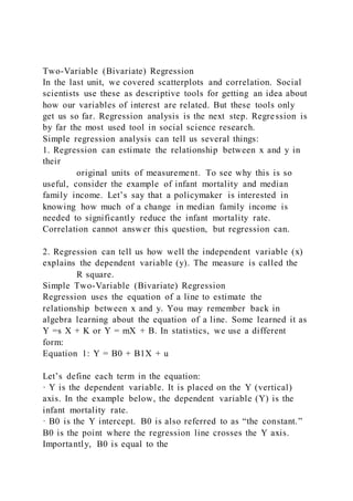
Using the AECF state data, the regression below measures the effect of the state's percentage of single parent families on the percentage of 4th graders with below basic reading scores.
%belowbasicread = β0 + β1x%SPF + u
Stata Output
1) Please write out the regression equation using the coefficients in the table
2) Please provide an interpretation of the coefficient for SPF
3) How does the model fit?
4) What is the NULL hypothesis for a T test about a regression coefficient?
5) What is the ALTERNATE hypothesis for a T test about a regression coefficient?
6) Look at the p value for the coefficient SPF.
a) Report the p value
b) How many stars would it get if we used our standard convention?
* p ≤ .1 ** p ≤ .05 *** p ≤ .01
image1.png
Two-Variable (Bivariate) Regression
In the last unit, we covered scatterplots and correlation. Social scientists use these as descriptive tools for getting an idea about how our variables of interest are related. But these tools only get us so far. Regression analysis is the next step. Regression is by far the most used tool in social science research.
Simple regression analysis can tell us several things:
1. Regression can estimate the relationship between x and y in their
original units of measurement. To see why this is so useful, consider the example of infant mortality and median family income. Let’s say that a policymaker is interested in knowing how much of a change in median family income is needed to significantly reduce the infant mortality rate. Correlation cannot answer this question, but regression can.
2. Regression can tell us how well the independent variable (x) explains the dependent variable (y). The measure is called the
R square.
Simple Tw ...
FSE 200AdkinsPage 1 of 10Simple Linear Regression Corr.docxbudbarber38650
FSE 200
Adkins Page 1 of 10
Simple Linear Regression
Correlation only measures the strength and direction of the linear relationship between two quantitative variables. If the relationship is linear, then we would like to try to model that relationship with the equation of a line. We will use a regression line to describe the relationship between an explanatory variable and a response variable.
A regression line is a straight line that describes how a response variable y changes as an explanatory variable x changes. We often use a regression line to predict the value of y for a given value of x.
Ex. It has been suggested that there is a relationship between sleep deprivation of employees and the ability to complete simple tasks. To evaluate this hypothesis, 12 people were asked to solve simple tasks after having been without sleep for 15, 18, 21, and 24 hours. The sample data are shown below.
Subject
Hours without sleep, x
Tasks completed, y
1
15
13
2
15
9
3
15
15
4
18
8
5
18
12
6
18
10
7
21
5
8
21
8
9
21
7
10
24
3
11
24
5
12
24
4
Draw a scatterplot and describe the relationship. Lay a straight-edge on top of the plot and move it around until you find what you think might be a “line of best fit.” Then try to predict the number of tasks completed for someone having been without sleep 16 hours.
Was your line the same as that of the classmate sitting next to you? Probably not. We need a method that we can use to find the “best” regression line to use for prediction. The method we will use is called least-squares. No line will pass exactly through all the points in the scatterplot. When we use the line to predict a y for a given x value, if there is a data point with that same x value, we can compute the error (residual):
Our goal is going to be to make the vertical distances from the line as small as possible. The most commonly used method for doing this is the least-squares method.
The least-squares regression line of y on x is the line that makes the sum of the squares of the vertical distances of the data points from the line as small as possible.
Equation of the Least-Squares Regression Line
· Least-Squares Regression Line:
· Slope of the Regression Line:
· Intercept of the Regression Line:
Generally, regression is performed using statistical software. Clearly, given the appropriate information, the above formulas are simple to use.
Once we have the regression line, how do we interpret it, and what can we do with it?
The slope of a regression line is the rate of change, that amount of change in when x increases by 1.
The intercept of the regression line is the value of when x = 0. It is statistically meaningful only when x can take on values that are close to zero.
To make a prediction, just substitute an x-value into the equation and find .
To plot the line on a scatterplot, just find a couple of points on the regression line, one near each end of the range of x in the data. Plot the points and connect them with a line. .
Data Science - Part XII - Ridge Regression, LASSO, and Elastic NetsDerek Kane
This lecture provides an overview of some modern regression techniques including a discussion of the bias variance tradeoff for regression errors and the topic of shrinkage estimators. This leads into an overview of ridge regression, LASSO, and elastic nets. These topics will be discussed in detail and we will go through the calibration/diagnostics and then conclude with a practical example highlighting the techniques.
For this assignment, use the aschooltest.sav dataset.The dMerrileeDelvalle969
For this assignment, use the aschooltest.sav dataset.
The dataset consists of Reading, Writing, Math, Science, and Social Studies test scores for 200 students. Demographic data include gender, race, SES, school type, and program type.
Instructions:
Work with the aschooltest.sav datafile and respond to the following questions in a few sentences. Please submit your SPSS output either in your assignment or separately.
1. Identify an Independent and Dependent Variable (of your choice) and develop a hypothesis about what you expect to find. (
note: the IV is a grouping variable, which means it needs to have more than 2 categories and the DV is continuous)
2. Run Assumption tests for Normality and initial Homogeneity of Variance. What are your results?
3. Run the one-way ANOVA with the Levene test & Tukey post hoc test.
a. What are the results of the Levene test? What does this mean?
b. What are the results of the one-way ANOVA (use notation)? What does it mean?
c. Are post hoc tests necessary? If so, what are the results of those analyses?
4. How do your analyses address your hypotheses?
Is concentration of single parent families associated with reading scores?
Using the AECF state data, the regression below measures the effect of the state's percentage of single parent families on the percentage of 4th graders with below basic reading scores.
%belowbasicread = β0 + β1x%SPF + u
Stata Output
1) Please write out the regression equation using the coefficients in the table
2) Please provide an interpretation of the coefficient for SPF
3) How does the model fit?
4) What is the NULL hypothesis for a T test about a regression coefficient?
5) What is the ALTERNATE hypothesis for a T test about a regression coefficient?
6) Look at the p value for the coefficient SPF.
a) Report the p value
b) How many stars would it get if we used our standard convention?
* p ≤ .1 ** p ≤ .05 *** p ≤ .01
image1.png
Two-Variable (Bivariate) Regression
In the last unit, we covered scatterplots and correlation. Social scientists use these as descriptive tools for getting an idea about how our variables of interest are related. But these tools only get us so far. Regression analysis is the next step. Regression is by far the most used tool in social science research.
Simple regression analysis can tell us several things:
1. Regression can estimate the relationship between x and y in their
original units of measurement. To see why this is so useful, consider the example of infant mortality and median family income. Let’s say that a policymaker is interested in knowing how much of a change in median family income is needed to significantly reduce the infant mortality rate. Correlation cannot answer this question, but regression can.
2. Regression can tell us how well the independent variable (x) explains the dependent variable (y). The measure is called the
R square.
Simple Tw ...
FSE 200AdkinsPage 1 of 10Simple Linear Regression Corr.docxbudbarber38650
FSE 200
Adkins Page 1 of 10
Simple Linear Regression
Correlation only measures the strength and direction of the linear relationship between two quantitative variables. If the relationship is linear, then we would like to try to model that relationship with the equation of a line. We will use a regression line to describe the relationship between an explanatory variable and a response variable.
A regression line is a straight line that describes how a response variable y changes as an explanatory variable x changes. We often use a regression line to predict the value of y for a given value of x.
Ex. It has been suggested that there is a relationship between sleep deprivation of employees and the ability to complete simple tasks. To evaluate this hypothesis, 12 people were asked to solve simple tasks after having been without sleep for 15, 18, 21, and 24 hours. The sample data are shown below.
Subject
Hours without sleep, x
Tasks completed, y
1
15
13
2
15
9
3
15
15
4
18
8
5
18
12
6
18
10
7
21
5
8
21
8
9
21
7
10
24
3
11
24
5
12
24
4
Draw a scatterplot and describe the relationship. Lay a straight-edge on top of the plot and move it around until you find what you think might be a “line of best fit.” Then try to predict the number of tasks completed for someone having been without sleep 16 hours.
Was your line the same as that of the classmate sitting next to you? Probably not. We need a method that we can use to find the “best” regression line to use for prediction. The method we will use is called least-squares. No line will pass exactly through all the points in the scatterplot. When we use the line to predict a y for a given x value, if there is a data point with that same x value, we can compute the error (residual):
Our goal is going to be to make the vertical distances from the line as small as possible. The most commonly used method for doing this is the least-squares method.
The least-squares regression line of y on x is the line that makes the sum of the squares of the vertical distances of the data points from the line as small as possible.
Equation of the Least-Squares Regression Line
· Least-Squares Regression Line:
· Slope of the Regression Line:
· Intercept of the Regression Line:
Generally, regression is performed using statistical software. Clearly, given the appropriate information, the above formulas are simple to use.
Once we have the regression line, how do we interpret it, and what can we do with it?
The slope of a regression line is the rate of change, that amount of change in when x increases by 1.
The intercept of the regression line is the value of when x = 0. It is statistically meaningful only when x can take on values that are close to zero.
To make a prediction, just substitute an x-value into the equation and find .
To plot the line on a scatterplot, just find a couple of points on the regression line, one near each end of the range of x in the data. Plot the points and connect them with a line. .
Data Science - Part XII - Ridge Regression, LASSO, and Elastic NetsDerek Kane
This lecture provides an overview of some modern regression techniques including a discussion of the bias variance tradeoff for regression errors and the topic of shrinkage estimators. This leads into an overview of ridge regression, LASSO, and elastic nets. These topics will be discussed in detail and we will go through the calibration/diagnostics and then conclude with a practical example highlighting the techniques.
30REGRESSION Regression is a statistical tool that a.docxtarifarmarie
30
REGRESSION
Regression is a statistical tool that allows you to predict the value of one continuous variable
from one or more other variables. When you perform a regression analysis, you create a
regression equation that predicts the values of your DV using the values of your IVs. Each IV is
associated with specific coefficients in the equation that summarizes the relationship between
that IV and the DV. Once we estimate a set of coefficients in a regression equation, we can use
hypothesis tests and confidence intervals to make inferences about the corresponding parameters
in the population. You can also use the regression equation to predict the value of the DV given a
specified set of values for your IVs.
Simple Linear Regression
Simple linear regression is used to predict the value of a single continuous DV (which we will
call Y) from a single continuous IV (which we will call X). Regression assumes that the
relationship between IV and the DV can be represented by the equation
Yi = β0 + β 1Xi + εi,
where Yi is the value of the DV for case i, Xi is the value of the IV for case i, β0 and β1 are
constants, and εi is the error in prediction for case i. When you perform a regression, what you
are basically doing is determining estimates of β0 and β1 that let you best predict values of Y
from values of X. You may remember from geometry that the above equation is equivalent to a
straight line. This is no accident, since the purpose of simple linear regression is to define the
line that represents the relationship between our two variables. β0 is the intercept of the line,
indicating the expected value of Y when X = 0. β1 is the slope of the line, indicating how much
we expect Y will change when we increase X by a single unit.
The regression equation above is written in terms of population parameters. That indicates that
our goal is to determine the relationship between the two variables in the population as a whole.
We typically do this by taking a sample and then performing calculations to obtain the estimated
regression equation
Yi = b0 + b1Xi .
Once you estimate the values of b0 and b1, you can substitute in those values and use the
regression equation to predict the expected values of the DV for specific values of the IV.
Predicting the values of Y from the values of X is referred to as regressing Y on X. When
analyzing data from a study you will typically want to regress the values of the DV on the values
of the IV. This makes sense since you want to use the IV to explain variability in the DV. We
typically calculate b0 and b1 using least squares estimation. This chooses estimates that minimize
the sum of squared errors between the values of the estimated regression line and the actual
observed values.
In addition to using the estimated regression equation for prediction, you can also perform
hypothesis tests regarding the individual regression parameters. The slope of the reg.
Regression Analysis presentation by Al Arizmendez and Cathryn LottierAl Arizmendez
We present an overview of regression analysis, theoretical construct, then provide a graphic representation before performing multiple regression analysis step by step using SPSS (audio files accompany the tutorial).
The future is uncertain. Some events do have a very small probabil.docxoreo10
The future is uncertain. Some events do have a very small probability of happening, like an asteroid destroying the earth. So we accept that tomorrow will come as a certain event. But future demand for a business’s goods and services is very uncertain. Yet, the management of a company wants to have some idea of the survival (or growth) of the company in the future. Should they expect to hire more people or let some go? Should they plan to increase capacity? How much investment is needed for future assets, or should they down size?
Forecasting provides some ideas about the future, but how this is accomplished can vary from company to company. And one key factor is how accurate the forecast is. Generally, the further into the future one looks, the more uncertain the information is. How do forecasters reduce their forecasting errors? How much error is tolerable?
Another key factor in forecasting is data availability. Data processing and storage capability have become extremely available and inexpensive. Software and computing power is also very cheap. Collecting real-time sales data via point-of-sales systems is now common at most retail establishments. But couple this with a situation in companies that have a large number of products, such as a retail store or a large manufacturing company with hundreds or thousands of product numbers and/or product lines, forecasting becomes complicated.
Forecasting Methods
There are two main types or genres of forecasting methods, qualitative and quantitative. The former consists of judgment and analysis of qualitative factors, such as scenario building and scenario analysis. The latter is obviously based on numerical analysis. This genre of forecasting includes such methods as linear regression, time series analysis, and data mining algorithms like CHAID and CART, which are useful especially in the growing world of artificial intelligence and machine learning in business. This module will look at the linear regression and time series analysis using exponential smoothing.
Linear Growth
When using any mathematical model, we have to consider which inputs are reasonable to use. Whenever we extrapolate, or make predictions into the future, we are assuming the model will continue to be valid. There are different types of mathematical model, one of which is linear growth model or algebraic growth model and another is exponential growth model, or geometric growth model. The constant change is the defining characteristic of linear growth. Plotting the values, we can see the values form a straight line, the shape of linear growth.
If a quantity starts at size P0 and grows by d every time period, then the quantity after n time periods can be determined using either of these relations:
Recursive form:
Pn = Pn-1 + d
Explicit form:
Pn = P0 + d n
In this equation, d represents the common difference – the amount that the population changes each time n increases by 1. Calculating values using the explicit form and plot ...
Introduction to linear regression and the maths behind it like line of best fit, regression matrics. Other concepts include cost function, gradient descent, overfitting and underfitting, r squared.
Linear regression is an approach for modeling the relationship between one dependent variable and one or more independent variables.
Algorithms to minimize the error are
OLS (Ordinary Least Square)
Gradient Descent and much more.
Let me know if anything is required. Ping me at google #bobrupakroy
Professional Memo 1 IFSM 201 Professional Memo .docxLacieKlineeb
Professional Memo 1
IFSM 201 Professional Memo
Before you begin this assignment, be sure you have read the Small Merchant Guide to Safe
Payments documentation from the Payment Card Industry Data Security Standards (PCI DSS)
organization. PCI Data Security Standards are established to protect payment account data
throughout the payment lifecycle, and to protect individuals and entities from the criminals who
attempt to steal sensitive data. The PCI Data Security Standard (PCI DSS) applies to all entities
that store, process, and/or transmit cardholder data, including merchants, service providers, and
financial institutions.
Purpose of this Assignment
You work as an Information Technology Consultant for the Greater Washington Risk Associates
(GWRA) and have been asked to write a professional memo to one of your clients as a follow-up
to their recent risk assessment (RA). GWRA specializes in enterprise risk management for state
agencies and municipalities. The county of Anne Arundel, Maryland (the client) hired GWRA to
conduct a risk assessment of Odenton, Maryland (a community within the Anne Arundel
County), with a focus on business operations within the municipality.
This assignment specifically addresses the following course outcome to enable you to:
• Identify ethical, security, and privacy considerations in conducting data and information
analysis and selecting and using information technology.
Assignment
Your supervisor has asked that the memo focus on Odenton’s information systems, and
specifically, securing the processes for payments of services. Currently, the Odenton Township
offices accept cash or credit card payment for the services of sanitation (sewer and refuse),
water, and property taxes. Residents can pay either in-person at township offices or over the
phone with a major credit card (American Express, Discover, MasterCard and Visa). Over the
phone payment involves with speaking to an employee and giving the credit card information.
Once payment is received, the Accounting Department is responsible for manually entering it
into the township database system and making daily deposits to the bank.
The purpose of the professional memo is to identify a minimum of three current controls
(e.g., tools, practices, policies) in Odenton Township (either a control specific to Odenton
Township or a control provided by Anne Arundel county) that can be considered best
practices in safe payment/data protection. Furthermore, beyond what measures are
currently in place, you should highlight the need to focus on insider threats and provide a
minimum of three additional recommendations. Below are the findings from the Risk
Assessment:
• The IT department for Anne Arundel County requires strong passwords for users to
access and use information systems.
https://www.pcisecuritystandards.org/pdfs/Small_Merchant_Guide_to_Safe_Payments.pdf
https://www.pcisec.
Principals in EpidemiologyHomework #2Please complete the fol.docxLacieKlineeb
Principals in Epidemiology
Homework #2
Please complete the following:
1. Utilizing the following list of communicable/infectious/exposure related conditions/diseases:
a. STI (Gonorrhea)
b. Hepatitis C
c. HIV (adult)
d. Tuberculosis
Please provide a description of the reporting requirements in
Virginia
and include all of the following elements for
each
of the above diseases (a-d).
Please include the name of the State, in the textbox above, in which you are providing information from and include all reference website URLs that the reporting information was obtained from for each disease below.
· Case definition: include suspect, probable, and/or confirmed, if appropriate
· Reporting criteria: time frame, method (e.g. by phone, Fax form, electronic), and required agency to report to (e.g. local HD, State HD, or CDC)
· Major elements of the information required to be reported (list categories or important information). If there is a
reporting form
availab1le, please attach a copy (
not all diseases have a manual reporting form or some forms are used for multiple diseases, only need to attach one copy and note which diseases utilize the same attached form
). If there is any standard follow-up patient/client information needed after reporting, please provide a description of this. If there is none, state this.
a. STI (Gonorrhea) –
b. Hepatitis C –
c. HIV (adult) –
d. Tuberculosis –
.
More Related Content
Similar to Two-Variable (Bivariate) RegressionIn the last unit, we covered
30REGRESSION Regression is a statistical tool that a.docxtarifarmarie
30
REGRESSION
Regression is a statistical tool that allows you to predict the value of one continuous variable
from one or more other variables. When you perform a regression analysis, you create a
regression equation that predicts the values of your DV using the values of your IVs. Each IV is
associated with specific coefficients in the equation that summarizes the relationship between
that IV and the DV. Once we estimate a set of coefficients in a regression equation, we can use
hypothesis tests and confidence intervals to make inferences about the corresponding parameters
in the population. You can also use the regression equation to predict the value of the DV given a
specified set of values for your IVs.
Simple Linear Regression
Simple linear regression is used to predict the value of a single continuous DV (which we will
call Y) from a single continuous IV (which we will call X). Regression assumes that the
relationship between IV and the DV can be represented by the equation
Yi = β0 + β 1Xi + εi,
where Yi is the value of the DV for case i, Xi is the value of the IV for case i, β0 and β1 are
constants, and εi is the error in prediction for case i. When you perform a regression, what you
are basically doing is determining estimates of β0 and β1 that let you best predict values of Y
from values of X. You may remember from geometry that the above equation is equivalent to a
straight line. This is no accident, since the purpose of simple linear regression is to define the
line that represents the relationship between our two variables. β0 is the intercept of the line,
indicating the expected value of Y when X = 0. β1 is the slope of the line, indicating how much
we expect Y will change when we increase X by a single unit.
The regression equation above is written in terms of population parameters. That indicates that
our goal is to determine the relationship between the two variables in the population as a whole.
We typically do this by taking a sample and then performing calculations to obtain the estimated
regression equation
Yi = b0 + b1Xi .
Once you estimate the values of b0 and b1, you can substitute in those values and use the
regression equation to predict the expected values of the DV for specific values of the IV.
Predicting the values of Y from the values of X is referred to as regressing Y on X. When
analyzing data from a study you will typically want to regress the values of the DV on the values
of the IV. This makes sense since you want to use the IV to explain variability in the DV. We
typically calculate b0 and b1 using least squares estimation. This chooses estimates that minimize
the sum of squared errors between the values of the estimated regression line and the actual
observed values.
In addition to using the estimated regression equation for prediction, you can also perform
hypothesis tests regarding the individual regression parameters. The slope of the reg.
Regression Analysis presentation by Al Arizmendez and Cathryn LottierAl Arizmendez
We present an overview of regression analysis, theoretical construct, then provide a graphic representation before performing multiple regression analysis step by step using SPSS (audio files accompany the tutorial).
The future is uncertain. Some events do have a very small probabil.docxoreo10
The future is uncertain. Some events do have a very small probability of happening, like an asteroid destroying the earth. So we accept that tomorrow will come as a certain event. But future demand for a business’s goods and services is very uncertain. Yet, the management of a company wants to have some idea of the survival (or growth) of the company in the future. Should they expect to hire more people or let some go? Should they plan to increase capacity? How much investment is needed for future assets, or should they down size?
Forecasting provides some ideas about the future, but how this is accomplished can vary from company to company. And one key factor is how accurate the forecast is. Generally, the further into the future one looks, the more uncertain the information is. How do forecasters reduce their forecasting errors? How much error is tolerable?
Another key factor in forecasting is data availability. Data processing and storage capability have become extremely available and inexpensive. Software and computing power is also very cheap. Collecting real-time sales data via point-of-sales systems is now common at most retail establishments. But couple this with a situation in companies that have a large number of products, such as a retail store or a large manufacturing company with hundreds or thousands of product numbers and/or product lines, forecasting becomes complicated.
Forecasting Methods
There are two main types or genres of forecasting methods, qualitative and quantitative. The former consists of judgment and analysis of qualitative factors, such as scenario building and scenario analysis. The latter is obviously based on numerical analysis. This genre of forecasting includes such methods as linear regression, time series analysis, and data mining algorithms like CHAID and CART, which are useful especially in the growing world of artificial intelligence and machine learning in business. This module will look at the linear regression and time series analysis using exponential smoothing.
Linear Growth
When using any mathematical model, we have to consider which inputs are reasonable to use. Whenever we extrapolate, or make predictions into the future, we are assuming the model will continue to be valid. There are different types of mathematical model, one of which is linear growth model or algebraic growth model and another is exponential growth model, or geometric growth model. The constant change is the defining characteristic of linear growth. Plotting the values, we can see the values form a straight line, the shape of linear growth.
If a quantity starts at size P0 and grows by d every time period, then the quantity after n time periods can be determined using either of these relations:
Recursive form:
Pn = Pn-1 + d
Explicit form:
Pn = P0 + d n
In this equation, d represents the common difference – the amount that the population changes each time n increases by 1. Calculating values using the explicit form and plot ...
Introduction to linear regression and the maths behind it like line of best fit, regression matrics. Other concepts include cost function, gradient descent, overfitting and underfitting, r squared.
Linear regression is an approach for modeling the relationship between one dependent variable and one or more independent variables.
Algorithms to minimize the error are
OLS (Ordinary Least Square)
Gradient Descent and much more.
Let me know if anything is required. Ping me at google #bobrupakroy
Professional Memo 1 IFSM 201 Professional Memo .docxLacieKlineeb
Professional Memo 1
IFSM 201 Professional Memo
Before you begin this assignment, be sure you have read the Small Merchant Guide to Safe
Payments documentation from the Payment Card Industry Data Security Standards (PCI DSS)
organization. PCI Data Security Standards are established to protect payment account data
throughout the payment lifecycle, and to protect individuals and entities from the criminals who
attempt to steal sensitive data. The PCI Data Security Standard (PCI DSS) applies to all entities
that store, process, and/or transmit cardholder data, including merchants, service providers, and
financial institutions.
Purpose of this Assignment
You work as an Information Technology Consultant for the Greater Washington Risk Associates
(GWRA) and have been asked to write a professional memo to one of your clients as a follow-up
to their recent risk assessment (RA). GWRA specializes in enterprise risk management for state
agencies and municipalities. The county of Anne Arundel, Maryland (the client) hired GWRA to
conduct a risk assessment of Odenton, Maryland (a community within the Anne Arundel
County), with a focus on business operations within the municipality.
This assignment specifically addresses the following course outcome to enable you to:
• Identify ethical, security, and privacy considerations in conducting data and information
analysis and selecting and using information technology.
Assignment
Your supervisor has asked that the memo focus on Odenton’s information systems, and
specifically, securing the processes for payments of services. Currently, the Odenton Township
offices accept cash or credit card payment for the services of sanitation (sewer and refuse),
water, and property taxes. Residents can pay either in-person at township offices or over the
phone with a major credit card (American Express, Discover, MasterCard and Visa). Over the
phone payment involves with speaking to an employee and giving the credit card information.
Once payment is received, the Accounting Department is responsible for manually entering it
into the township database system and making daily deposits to the bank.
The purpose of the professional memo is to identify a minimum of three current controls
(e.g., tools, practices, policies) in Odenton Township (either a control specific to Odenton
Township or a control provided by Anne Arundel county) that can be considered best
practices in safe payment/data protection. Furthermore, beyond what measures are
currently in place, you should highlight the need to focus on insider threats and provide a
minimum of three additional recommendations. Below are the findings from the Risk
Assessment:
• The IT department for Anne Arundel County requires strong passwords for users to
access and use information systems.
https://www.pcisecuritystandards.org/pdfs/Small_Merchant_Guide_to_Safe_Payments.pdf
https://www.pcisec.
Principals in EpidemiologyHomework #2Please complete the fol.docxLacieKlineeb
Principals in Epidemiology
Homework #2
Please complete the following:
1. Utilizing the following list of communicable/infectious/exposure related conditions/diseases:
a. STI (Gonorrhea)
b. Hepatitis C
c. HIV (adult)
d. Tuberculosis
Please provide a description of the reporting requirements in
Virginia
and include all of the following elements for
each
of the above diseases (a-d).
Please include the name of the State, in the textbox above, in which you are providing information from and include all reference website URLs that the reporting information was obtained from for each disease below.
· Case definition: include suspect, probable, and/or confirmed, if appropriate
· Reporting criteria: time frame, method (e.g. by phone, Fax form, electronic), and required agency to report to (e.g. local HD, State HD, or CDC)
· Major elements of the information required to be reported (list categories or important information). If there is a
reporting form
availab1le, please attach a copy (
not all diseases have a manual reporting form or some forms are used for multiple diseases, only need to attach one copy and note which diseases utilize the same attached form
). If there is any standard follow-up patient/client information needed after reporting, please provide a description of this. If there is none, state this.
a. STI (Gonorrhea) –
b. Hepatitis C –
c. HIV (adult) –
d. Tuberculosis –
.
Prevalence Of Pressure Ulcer Name xxxUnited State Universit.docxLacieKlineeb
Prevalence Of Pressure Ulcer
Name xxx
United State University
Course xxxx
Professor xxxx
The Prevalence of Pressure Ulcer Among The Elderly And Decreased Mobility Patients in The Hospitals And Healthcare Facilities.
Abstract
Hospital-acquired pressure ulcers remain to be amongst the continuous and persistent healthcare issues that are affecting the delivery of quality healthcare services. Pressure ulcers or pressure sores or bedsores refer to the injuries of the skin and the underlying tissues that are mainly caused by the prolonged pressure on the skin. According to the National Health Service, these conditions are common in individuals who are bedridden or are sitting on wheelchairs and chairs for an extended period. The disease occurs on the body parts that are commonly exposed to the pressure for example the spine, hips, elbows, and heels. The issue of pressure ulcers is a major public health concern since it consumes large sums of money to address the problem (Grey et al., 2016). On average, a client is being charged $ 37,800 for extreme cases of pressure ulcers.
This study aims to implement certain method to prevent pressure ulcers among the elderly above 60 years and decreased mobility patients in the hospital and healthcare facilities through the use of Braden scale, applying mepilex foam dressing to bony prominence areas, and repositioning. Patients especially elderly adults are experiencing lengthy hospital stays and this is exposing them to the high risk of pressure ulcers. According to Rondinelli et al (2018), several factors are linked to pressure ulcers. These multi-factorial factors involve hormonal changes, impairment of blood perfusion, inflammation, degenerative changes, and reduction in the effectiveness of immunity. The majority of elderly patients suffer from frailty and other chronic diseases that reduce their ability to engage in daily activities (ADLs) and even experiences limited movements. This increases their level of exposure to hospital-acquired pressure injury (HAPI). This is a health concern that requires the development of effective evidence-based interventions to help in the creation of awareness concerning therapy and preventive approaches such as the application of the Braden Scale to help in detecting the risks of adult patients. It is also important to design approaches that are helpful in the protection of the bony regions using pads and repositioning of the patients after every 2 hours (Lyder & Ayello, 2018).
Many healthcare facilities have attempted to design effective evidence-based interventions but the issue of healthcare-acquired pressure ulcers continued to persist. Despite the increased efforts to implement evidence-based procedures to guide the nurses in reducing the pressure ulcers issue within the acute care facilities, the number of reported cases of pressure ulcers continues to be a major issue (Grey et al., 2016). The majority of healthcare facilities are fa.
Professional Disposition and Ethics - Introduction kthometz post.docxLacieKlineeb
Professional Disposition and Ethics - Introduction
kthometz posted on 09-27-2022 11:26 AM 10-25-2022 06:18 PM
WGU’s mission is to “change lives for the better by creating pathways to opportunity.” Teachers College Way is to “change lives for the better by catalyzing Next-Gen teaching, learning, and leading across the education spectrum.
Next-Gen Candidates
A Next-Gen candidate is transformative in teaching, learning, and leading across the education spectrum. Teachers College strives to foster organizational systems and culture that allow candidates, faculty, and staff to do their life’s best work. Next-generation education begins with the core belief that the art and science of teaching, learning, and leading in education must continually evolve, becoming better and better with each subsequent generation. Catalyzing Next-Gen teaching, learning, and leading requires experience in a transformative educational environment.
Healthy Learning
Teachers College endeavors to offer a healthy learning environment that supports the professional growth and development of each Next-Gen candidate and expands the professional opportunities for each Next-Gen graduate. The development of Professional Dispositions and Ethics for Next-Gen candidates strengthens the educational experience and conveys the Teachers College’s commitment to impactful teaching, learning, and leading to the greater professional community.
A vital aspect of transforming Professional Dispositions and Ethics is the integration of restorative practices. Next-Gen candidates are empowered to use effective, evidence-based best practices to create healthy learning environments where all learners rise and thrive. Teachers College provides candidates with a safe educational environment - a place where candidates can develop and strengthen their academic, physical, psychological, ethical, and social understandings (learn more about
Healthy Learning). Our Professional Dispositions and Ethics at WGU is supported by the five primary critical healthy-learning focus areas that are key drivers of learner academic, professional, and personal success. These five pillars, while being powerful concepts individually, gain collective strength and create a thriving, healthy learning environment, where all individuals are equipped to fully embody and practice Teachers College Professional Disposition and Ethics.
The five pillars of Healthy Learning are:
1. Diversity, Equity, and Inclusion (DE&I)
2. Social-Emotional Learning (SEL)
3. Character Education
4. Mental Health
5. Basic Needs
Figure 1
Figure 1:This graphic represents the research, reflection, policy & practice impact the five pillars of Healthy Learning. This figure shows that the five pillars of Healthy Learning are interconnected.
Diversity, equity, and inclusion (DE&I) impact all spaces within education. It is vital to address ongoing challenges of the inequalities of access and attainment am.
Problem 7PurposeBreak apart a complicated system.ConstantsC7C13.docxLacieKlineeb
Problem 7Purpose:Break apart a complicated system.Constants:C7:C13Gas-Sparge
System
Pmo794(DI/DT)^4.38DI0.36(DI2N/v)^0.115DT1.22(DIN2/g)^1.96(DI/Dt)N2.8(Q/NDI3)v8.90E-07Right Sideg9.81PM←ANSWERSQ0.00416Computed Pm917The difference between the Computed Pm and Calculated Pm
Problem 8Purpose:Calculate Wind ChillConstants:ParametersWind Speed (km/h)a13.12Air Temp oC1020304050b0.621510c-11.370d0.3965-10-20←ANSWERS-30-40QuestionsThe formula to be used in E5 such that it can be filled down and across to make the table is: ….The name for cell B6 is …To modify this worksheet for Fahrenheit you need to …..
Problem 13Purpose:Calculate square roots using Heron's MethodConstants:N225Sqrt is←ANSWERSGuessN/GuessAverageTestError10
2
Project Topic Proposal
Harita Patel
Professor Dr. Bernard Parenteau
CIS 4498
Date: 11/1/22
Project Topic Proposal
The proposed topic is cyber security. My proposal in this software development project of this class is to develop cyber security software to be a tool that protects systems against malicious attacks and online threats. The software should b able to detect and block threats that can not be detected by antivirus. The technology to be used will be defensive Artificial intelligence. Cybersecurity professional experts can utilize guarded man-made consciousness (simulated intelligence) to distinguish or stop cyberattacks. Sagacious cybercriminals use innovations like hostile computer-based intelligence and ill-disposed AI since they are harder for conventional network protection instruments to identify. Offensive AI incorporates profound fakes, bogus pictures, personas, and recordings that convincingly portray individuals or things that never occurred or don't exist. Noxious entertainers can utilize ill-disposed AI to fool machines into breaking down by giving them mistaken information. Cybersecurity professionals can utilize cautious computer-based intelligence to recognize and prevent hostile man-made intelligence from estimating, testing, and figuring out how the framework or organization's capabilities. Defensive AI can reinforce calculations, making them more challenging to break. Network protection analysts can direct more extreme weakness tests on AI models.
Artificial intelligence cautious apparatuses can precisely anticipate assault vectors, pinpoint the delicate region of the organization and frameworks, and even set it up groups for approaching occasions(Graham, Olson,& Howard, 2016). The progression of computerized data is developing a regular schedule making it progressively challenging to oversee and structure it or even to isolate what is significantly based on what is pointless. Confronted with this test, new encouraging advancement innovations are being created to bring 'information examination's to the following developmental level. Man-made consciousness (man-made intelligence), specifically, is supposed to become huge in many fields. A few types of computer-based inte.
Procedure1. Research occupation as it relates to Occupati.docxLacieKlineeb
Procedure
:
1. Research occupation as it relates to Occupational Therapy
2. Provide statistics, tests, and measurements for the purpose of delivering evidence-based practice and/or service delivery options as it relates to occupation.
3. Adapt the presentation for the following:
a. Consumers
b. Potential employers
c. Colleagues
d. Third Party Payers
e. Regulatory Boards
f. Policy Makers
4. You will present this information to the class in the form of a power point presentation and each slide should be labeled with for your target audience.
.
Problem 1 (10 Points)Jackson Browne Corporation is authorized to.docxLacieKlineeb
Problem 1 (10 Points)
Jackson Browne Corporation is authorized to issue 1,000,000 shares of $1 par value common stock. During 2021, its first year of operation, the company has the following stock transactions.
Jan. 1 Paid the state $10,000 for incorporation fees.
Jan. 15 Issued 400,000 shares of stock at $5 per share.
July 2 Issued 110,000 shares of stock for land. The land had an asking price of $800,000. The stock is currently selling on a national exchange at $6 per share.
Sept. 5 Purchased 12,000 shares of common stock for the treasury at $7 per share.
Dec. 6 Sold 8,000 shares of the treasury stock at $10 per share.
Instructions
Indicate the accounts and their respective balances that are increased and/or decreased in the above transactions for Jackson Browne Corporation.
You must show your computations to receive full credit.
Problem 2 (12 Points)
The following items were shown on the balance sheet of ELO Corporation on December 31, 2021:
Stockholders’ equity
Paid-in capital
Capital stock
Common stock, $6 par value, 800,000 shares
authorized; ______ shares issued and ______ outstanding $3,000,000
Additional paid-in capital
In excess of par
1,500,000
Total paid-in capital 4,500,000
Retained earnings
1,850,000
Total paid-in capital and retained earnings 6,350,000
Less: Treasury stock (10,000 shares)
50,000
Total stockholders’ equity
$6,300,000
Instructions
Complete the following statements and
show your computations.
(a) The number of shares of common stock issued was _______________.
(b) The number of shares of common stock outstanding was ____________.
(c) The total sales price of the common stock when issued was $____________.
(d) The cost per share of the treasury stock was $_______________.
(e) The average issue price of the common stock was $______________.
(f) Assuming that 25% of the treasury stock is sold at $8 per share, the balance in the Treasury Stock account would be $_______________.
Problem 3 (10 Points)
Journey Company had the following transactions involving notes payable.
October 1, 2021 Borrows $300,000 from Washington State Bank by signing a 6-month, 4% note.
Dec. 31, 2021 prepares the adjusting entry.
April 1, 2022 Pays principal and interest to Washington State Bank.
Instructions
Indicate the accounts and their respective balances that are increased and/or decreased for each of the above transactions.
You must show all your calculations to receive full credit.
Problem 4 (18 Points)
Turner Inc. is considering two alternatives to finance its construction of a new $6 million plant.
(a) Issuance of 600,000 shares of common stock at the market price of $10 per share.
(b) Issuance of $6 million, 4% bonds at par.
Instructions
Complete the following table.
You MUST show your work to receive full credit.
Issue StockIssue Bond.
Primary Task Response Within the Discussion Board area, write 350.docxLacieKlineeb
Primary Task Response:
Within the Discussion Board area, write 350–450 words that respond to the following questions with your thoughts, ideas, and comments. This will be the foundation for future discussions by your classmates. Be substantive and clear, and use examples to reinforce your ideas.
Additional Information:
Eddison Electronic Company (EEC) provides electricity for several states in the United States. You have been employed as a cost accountant at this organization. You have recently hired Susan Thompson, who has experience with financial accounting. Financial accounting includes preparing journal entries that provide a record of the day-to-day activities of the company and preparing financial statements, such as an income statement, a statement of owners’ equity balance sheet, and a cash flow statement. Although Susan has experience with and fully understands financial accounting, she has no experience with managerial accounting.
With your fellow classmates, please discuss what Susan should know about managerial accounting.
Explain the similarities and differences between financial and managerial accounting.
Provide examples of the reports used for financial reporting and how those reports differ from managerial accounting reports.
Determine how managers might use accounting information for planning and controlling purposes.
.
Principles of Scientific Management, Frederick Winslow Taylor .docxLacieKlineeb
Principles of Scientific Management, Frederick Winslow Taylor (1911)
Introduction
PRESIDENT ROOSEVELT, in his address to the Governors at the White House,
prophetically remarked that “The conservation of our national resources is only preliminary to
the larger question of national efficiency.”
The whole country at once recognized the importance of conserving our material
resources and a large movement has been started which will be effective in accomplishing this
object. As yet, however, we have but vaguely appreciated the importance of “the larger question
of increasing our national efficiency.”
We can see our forests vanishing, our water-powers going to waste, our soil being carried
by floods into the sea; and the end of our coal and our iron is in sight. But our larger wastes of
human effort, which go on every day through such of our acts as are blundering, ill-directed; or
inefficient, and which Mr. Roosevelt refers to as a lack of “national efficiency,” are less visible,
less tangible, and are but vaguely appreciated.
We can see and feel the waste of material things. Awkward, inefficient, or ill-directed
movements of men, however, leave nothing visible or tangible behind them. Their appreciation
calls for an act of memory, an effort of the imagination. And for this reason, even though our
daily loss from this source is greater than from our waste of material things, the one has stirred
us deeply, while the other has moved us but little.
As yet there has been no public agitation for “greater national efficiency,” no meetings
have been called to consider how this is to be brought about. And still there are signs that the
need for greater efficiency is widely felt.
The search for better, for more competent men, from the presidents of our great
companies down to our household servants, was never more vigorous than it is now. And more
than ever before is the demand for competent men in excess of the supply.
What we are all looking for, however, is the readymade, competent man; the man whom
some one else has trained. It is only when we fully realize that our duty, as well as our
opportunity, lies in systematically cooperating to train and to make this competent man, instead
of in hunting for a man whom some one else has trained, that we shall be on the road to national
efficiency.
In the past the prevailing idea has been well expressed in the saying that “Captains of
industry are born, not made”; and the theory has been that if one could get the right man,
methods could be safely left to him. In the future it will be appreciated that our leaders must be
trained right as well as born right, and that no great man can (with the old system of personal
management) hope to compete with a number of ordinary men who have been properly
organized so as efficiently to cooperate.
In the past the man has been first; in the future the system must be first. This in no sense,
.
Printed by [email protected] Printing is for personal, privat.docxLacieKlineeb
Printed by: [email protected] Printing is for personal, private use only. No part of this book may be
reproduced or transmitted without publisher's prior permission. Violators will be prosecuted.
Printed by: [email protected] Printing is for personal, private use only. No part of this book may be
reproduced or transmitted without publisher's prior permission. Violators will be prosecuted.
Printed by: [email protected] Printing is for personal, private use only. No part of this book may be
reproduced or transmitted without publisher's prior permission. Violators will be prosecuted.
Printed by: [email protected] Printing is for personal, private use only. No part of this book may be
reproduced or transmitted without publisher's prior permission. Violators will be prosecuted.
Printed by: [email protected] Printing is for personal, private use only. No part of this book may be
reproduced or transmitted without publisher's prior permission. Violators will be prosecuted.
Printed by: [email protected] Printing is for personal, private use only. No part of this book may be
reproduced or transmitted without publisher's prior permission. Violators will be prosecuted.
Printed by: [email protected] Printing is for personal, private use only. No part of this book may be
reproduced or transmitted without publisher's prior permission. Violators will be prosecuted.
Due Date: 11:59 pm EST Sunday of Unit 4
Points: 100
Overview:
In this assignment, you will review Case Study #12: SpaceX. This case describes Elon
Musk’s unique approach to strategy when creating SpaceX. Think about the types of
strategies from chapters 5 and 6 that Elon Musk utilized.
Instructions:
You will need to review the case study in your textbook, then answer the following
questions utilizing topics covered in previous chapters.
• What were Elon Musk’s motives for creating SpaceX? How do these motives
influence the kinds of decisions he made in creating the firm?
• Thinking about Musk’s prior experiences, capabilities, and motives, what do you
think are his strengths and weaknesses in creating SpaceX?
• What did SpaceX do differently from other space companies?
• Discuss whether you believe the incumbent space companies will adopt
elements of SpaceX’s model (be specific about which). Do you think the
incumbents will survive? Do you believe Jeff Bezos’s Blue Origin is a significant
threat?
Requirements:
• Submit a two-three page Word document covering the elements of the
assignment.
• Develop a clear introduction, body, and conclusion. Use paragraph format and
transitions.
• Focus on the quality of writing and content.
• Use APA format with a title page, in-text citations, and references. Abstract is not
required. The title page, reference page, and appendices are excluded in page
length requirement.
• Research and cite at least two credible sources in APA format.
Be sure to read the criteria below.
Primary Care Integration in Rural AreasA Community-Focused .docxLacieKlineeb
Primary Care Integration in Rural Areas:
A Community-Focused Approach
Emily M. Selby-Nelson, PsyD
Cabin Creek Health Systems, Charleston,
West Virginia
Joshua M. Bradley, PsyD
Tri-Area Community Health, Laurel Fork, Virginia
Rebekah A. Schiefer, MSW
Oregon Health & Science University
Alysia Hoover-Thompson, PsyD
Stone Mountain Health Services,
Jonesville, Virginia
Current and developing models of integrated behavioral health service delivery have
proven successful for the general population; however, these approaches may not
sufficiently address the unique needs of individuals living in rural and remote areas. For
all communities to benefit from the opportunities that the current trend toward inte-
gration has provided, it is imperative that cultural and contextual factors be considered
determining features in care delivery. Rural integrated primary care practice requires
specific training, expertise, and adjustments to service delivery and intervention to best
meet the needs of rural and underserved communities. In this commentary, the authors
present trends in integrated behavioral health service delivery in rural integrated
primary care settings. Flexible and creative strategies are proposed to promote in-
creased access to integrated behavioral health services, while simultaneously address-
ing patient care needs that arise as a result of the barriers to treatment that are prevalent
in rural communities.
Keywords: integrated behavioral health, integrated primary care, rural, rural health
The need for integrated health care is well
documented. Nearly 70% of primary care ap-
pointments include issues associated with psy-
chosocial factors (Gatchel & Oordt, 2003).
Many patients would prefer to receive behav-
ioral health services in their primary care pro-
vider’s office, as opposed to a specialty mental
health setting (Lang, 2005). Patients in primary
care offices are also more likely to follow
through with a behavioral health referral when
that service is provided in the same office (Slay
& McCleod, 1997). Overall, integrated behav-
ioral health services have been shown to suc-
cessfully enhance health care services and yield
improvements in medical and behavioral health
conditions (Kwan & Nease, 2013).
Integrated care models may be especially im-
pactful in areas where access to specialty care is
limited, such as rural communities. However, a
discussion of the adjustments warranted when
developing integrated behavioral health ser-
vices in rural practice settings is all but absent in
the literature. Significant treatment needs in ru-
ral areas, combined with poor availability of
referral-based services in rural communities, re-
quire effective integrated primary care (IPC) to
be provided in a flexible, patient-tailored, and
community-focused manner. In this paper, we
aim to outline the special considerations neces-
sary for conducting IPC in rural communities
wherein behavioral health providers (BHPs)
may struggle to balance in.
PrepareStep 1 Prepare a shortened version of your Final Pape.docxLacieKlineeb
Prepare:
Step 1: Prepare a shortened version of your Final Paper (at least four pages) by including the following:
Introduction paragraph and thesis statement you developed for your Week 3 Assignment.
Background information of the global societal issue you have chosen.
Brief argument supporting at least two solutions to the global societal issue.
Conclusion paragraph.
Must document any information used from at least five scholarly sources in APA style as outlined in the University of Arizona Global Campus Writing Center’s Citing Within Your PaperLinks to an external site. Note that you will need at least eight scholarly sources for your Final Paper in Week 5.
Final paper
Write: This Final Paper, an argumentative essay, will present research relating the critical thinker to the modern, globalized world. In this assignment, you need to address the items below in separate sections with new headings for each.
In your paper,
Identify the global societal problem within the introductory paragraph.
Conclude with a thesis statement that states your proposed solutions to the problem. (For guidance on how to construct a good introduction paragraph, please review the Introductions & ConclusionsLinks to an external site. from the University of Arizona Global Campus Writing CenterLinks to an external site..)
Describe background information on how that problem developed or came into existence.
Show why this is a societal problem.
Provide perspectives from multiple disciplines or populations so that you fully represent what different parts of society have to say about this issue.
Construct an argument supporting your proposed solutions, considering multiple disciplines or populations so that your solution shows that multiple parts of society will benefit from this solution.
Provide evidence from multiple scholarly sources as evidence that your proposed solution is viable.
Interpret statistical data from at least three peer-reviewed scholarly sources within your argument.
Discuss the validity, reliability, and any biases.
Identify the strengths and weaknesses of these sources, pointing out limitations of current research and attempting to indicate areas for future research. (You may even use visual representations such as graphs or charts to explain statistics from sources.)
Evaluate the ethical outcomes that result from your solution.
Provide at least one positive ethical outcome as well as at least one negative ethical outcome that could result from your solution.
Explain at least two ethical issues related to each of those outcomes. (It is important to consider all of society.)
Develop a conclusion for the last paragraphs of the essay, starting with rephrasing your thesis statement and then presenting the major points of the topic and how they support your argument. (For guidance on how to write a good conclusion paragraph, please review the Introductions & ConclusionsLinks to an external site. from the University of Arizona Global Campus Writing Cente.
Princess Nourah bint Abdulrahman University Strategy and Ope.docxLacieKlineeb
Princess Nourah bint Abdulrahman University
Strategy and Operations Consulting Seminar: Open Cases
October 2022
Case 1: Supply Chain Optimization in the Dairy Sector 3
▪ Context
▪ Data to consider
▪ Questions to solve
Case 2: Business Case for an Investment Opportunity in Real Estate 18
Case 3: Financial Valuation for a Renewable Energy Start-up 22
Annex 31
2PNU – Strategy and Operations Consulting Seminar
INDEX
An important group in the dairy sector of the Basque Country. “Lácteos SA”. carries
out the distribution of all kinds of food products to the different distribution
channels: Food and HORECA
FOOD DRY SMOOTHIES BEVERAGES
DERIVATIVES SWEET SAUSAGES
MILK MILK POWDER SINGLE DOSE
CHEESES WITHOUT
LACTOSE YOGURT
product familiesmain channels
Total References: 510
29,4%
7,2% 4,8%
22,2%
35,6%
0,8%
0,0%
10,0%
20,0%
30,0%
40,0%
50,0%
Frío Seco Din
41,4%
58,6%
Kaiku
Km0
Food
HORECA
References
(in number of references)
Open case 1. Context
PNU – Strategy and Operations Consulting Seminar 3
own
product
external
product
Cold Dry
I
The current flow of the distribution process of Lácteos SA entails the passage
of most of the product through the central platform located in Jundiz (Basque
Country)
From there it is distributed to Food customers. and the Horeca channel (food service) both directly and through its
delegations.
Location of delegations
Biscay
Gipuzkoa
Araba-Jundiz
Navarre
Cantabria
Rioja Barcelona
Zaragoza
Valencia
Madrid
Current Flow of the Distribution Process
Other Manufacturers/
external suppliers
Central
platform
Jundiz
Food
Horeca Channel
Delegations
Manufacturers/
Suppliers own self
of Lácteos SA
PNU – Strategy and Operations Consulting Seminar 4
Open case 1. Context
Central platform
Jundiz
The current network of Lácteos SA has 64 origins and 1.120
destinations of the Jundiz platform
64 Origins 1.120 destinations664.316 lines prepared
48.636 orders prepared
560 Food destinations
550 Horeca destinations
10 Delegations
Own factories of
Lácteos SA
5
15 own suppliers of
Lácteos SA
45 external suppliers
PNU – Strategy and Operations Consulting Seminar 5
Open case 1. Context
PNU – Strategy and Operations Consulting Seminar 6
In this background, the client requests…
Project Objectives
… to carry out a diagnosis of the current logistics model to carry out the appropriate network design
for current and future market demand, considering the possibility of separating or outsourcing certain
channels
▪ Dimensioning of the network from the production centres and external suppliers to the distribution carried out from
the distribution centre of Jundiz
▪ Distribution system sizing. current scenario vs. other possible scenarios
▪ Cost evaluation of scenarios based on ratios available by Lácteos SA: cost €/km by type of vehicle. cost €/m2 of
warehouse by location…
Open case 1. Context
PNU – Strategy and Operations Consulting Seminar 7
In o.
Primary Care Interventions for Prevention and Cessation of Tob.docxLacieKlineeb
Primary Care Interventions for Prevention and Cessation of Tobacco Use
in Children and Adolescents
US Preventive Services Task Force Recommendation Statement
US Preventive Services Task Force
Summary of Recommendations
The USPSTF recommends that primary care clinicians provide interventions, including education or
brief counseling, to prevent initiation of tobacco use among school-aged children and adolescents. B
The USPSTF concludes that the current evidence is insufficient to assess the balance of benefits and
harms of primary care–feasible interventions for the cessation of tobacco use among school-aged
children and adolescents.
I
See the Figure for a more detailed summary of the recommendation for clinicians. See the Practice Considerations section for more information on effective
interventions to prevent initiation of tobacco use and for suggestions for practice regarding the I statement. USPSTF indicates US Preventive Services Task Force.
IMPORTANCE Tobacco use is the leading cause of preventable death in the US. An estimated
annual 480 000 deaths are attributable to tobacco use in adults, including from secondhand
smoke. It is estimated that every day about 1600 youth aged 12 to 17 years smoke their first
cigarette and that about 5.6 million adolescents alive today will die prematurely from a
smoking-related illness. Although conventional cigarette use has gradually declined among
children in the US since the late 1990s, tobacco use via electronic cigarettes (e-cigarettes) is
quickly rising and is now more common among youth than cigarette smoking. e-Cigarette
products usually contain nicotine, which is addictive, raising concerns about e-cigarette use
and nicotine addiction in children. Exposure to nicotine during adolescence can harm the
developing brain, which may affect brain function and cognition, attention, and mood; thus,
minimizing nicotine exposure from any tobacco product in youth is important.
OBJECTIVE To update its 2013 recommendation, the USPSTF commissioned a review of the
evidence on the benefits and harms of primary care interventions for tobacco use prevention
and cessation in children and adolescents. The current systematic review newly included
e-cigarettes as a tobacco product.
POPULATION This recommendation applies to school-aged children and adolescents younger
than 18 years.
EVIDENCE ASSESSMENT The USPSTF concludes with moderate certainty that primary
care–feasible behavioral interventions, including education or brief counseling, to prevent
tobacco use in school-aged children and adolescents have a moderate net benefit. The
USPSTF concludes that there is insufficient evidence to determine the balance of benefits
and harms of primary care interventions for tobacco cessation among school-aged children
and adolescents who already smoke, because of a lack of adequately powered studies on
behavioral counseling interventions and a lack of studies on medications.
RECOMMENDATION The USPSTF recommends that.
Presentation given in 2 separate PP documents as example.8-10 .docxLacieKlineeb
Presentation given in 2 separate PP documents as example.
8-10 slides on PowerPoint Topic (Cover Page and Reference Page EXCLUDED)
Topic: Post Partum Hemorrhage PPH Note: I have the content
Must use 2-3 scholarly articles from LEARN (Given when Bid accepted)
2-3 in-text APA Citations (Citationmachine.net)
Turn In It score MUST be less than 20%
Slides must include
Etiology,
Nursing Interventions,
Patient Education,
Treatment (if applicable).
Link a video in the last page as reference
First PP colors and presentation on file
Second PP given with the content
.
Prepare a PowerPoint presentation (8 slides minimum) that presents a.docxLacieKlineeb
Prepare a PowerPoint presentation (8 slides minimum) that presents a synopsis of an article from a peer- reviewed academic journal. The article should focus on "organizational leadership topic". The article needs to have been published within the past 10 years.
You are ONLY supposed to review ONE article which is related to organizational leadership.
.
PRAISE FOR CRUCIAL CONVERSATIONS Relationships ar.docxLacieKlineeb
PRAISE FOR CRUCIAL CONVERSATIONS
"Relationships are the priority of life, and conversations are the
crucial element in profound caring of relationships. This book
helps us to think about what we really want to say. If you want
to succeed in both talking and listening, read this book."
-Dr. Lloyd J. Ogilvie, chaplain, United States Senate
"Important, lucid, and practical, Crucial Conversations is a
book that will make a difference in your life. Learn how to flour
ish in every difficult situation."
-Robert E. Quinn, ME Tracy Collegiate Professor of
OBHRM, University of Michigan Business School
"I was personally and professionally inspired by this book-and
I'm not easily impressed. In the fast-paced world of IT, the success
of our systems, and our business, depends on crucial conversations
we have every day. Unfortunately, because our environment is so
technical, far too often we forget about the 'human systems' that
make or break us. These skills are the missing foundation piece."
-Maureen Burke, manager of training,
Coca-Cola Enterprises, Inc.
"The book is compelling. Yes, I found myself in too many of their
examples of what not to do when caught in these worst-of-all
worlds situations! GET THIS BOOK, WHIP OUT A PEN AND
GET READY TO SCRIBBLE MARGIN NOTES FURIOUSLY,
AND PRACTICE, PRACTICE, PRACTICE THE INVALUABLE
TOOLS THESE AUTHORS PRESENT. I know I did-and it
helped me salvage several difficult situations and repair my
damaged self-esteem in others. I will need another copy pretty
soon. as I'm wearing out the pages in this one!"
-James Belasco. best-selling author of Flight of the Buffalo,
l!l1trl!prl!l1eur. professor. und l!xl!cutive director of the Financial
Tilllrs Knowkdgc Diuloguc
"Crucial Conversations is the most useful self-help book I have
ever read. I'm awed by how insightful, readable, well organized,
and focused it is. I keep thinking: 'If only I had been exposed to
these dialogue skills 30 years ago ... '"
-John Hatch, founder, FINCA International
"One of the greatest tragedies is seeing someone with incredible
talent get derailed because he or she lacks some basic skills.
Crucial Conversations addresses the number one reason execu
tives derail, and it provides extremely helpful tools to operate in
a fast-paced, results-oriented environment."
-Karie A. Willyerd, chief talent officer, Solectron
"The book prescribes, with structure and wit, a way to improve on
the most fundamental element of organizational learning and
growth-honest, unencumbered dialogue between individuals.
There are one or two of the many leadership/management
'thought' books on my shelf that are frayed and dog-eared from
use. Crucial Conversations will no doubt end up in the same con
dition."
-John Gill, VP of Human Resources, Rolls Royce USA
Crucial
Conversations
Crucial
Conversations
Tools for Talking
When Stakes Are High
by
Kerry Patterson, .
Porwerpoint The steps recommended for efficiently developing an ef.docxLacieKlineeb
Porwerpoint : The steps recommended for efficiently developing an effective and consistent PowerPoint presentation include: 1.planning, 2.entering content, 3.editing, 4.formatting, 5.previewing, and 6.delivering (e.g. print, email, publish). Identify a key consideration one should make when planning a PowerPoint presentation? Describe the differences between building slide shows from blank presentations, themes, and templates. Discuss how PowerPoint presentations can be used both professionally and personally.
100 words minimum
.
Prepare a 2-page interprofessional staff update on HIPAA and appro.docxLacieKlineeb
Prepare a 2-page interprofessional staff update on HIPAA and appropriate social media use in health care.
Introduction
As you begin to consider the assessment, it would be an excellent choice to complete the Breach of Protected Health Information (PHI) activity. The activity will support your success with the assessment by creating the opportunity for you to test your knowledge of potential privacy, security, and confidentiality violations of protected health information. The activity is not graded and counts towards course engagement.
Health professionals today are increasingly accountable for the use of protected health information (PHI). Various government and regulatory agencies promote and support privacy and security through a variety of activities. Examples include:
· Meaningful use of electronic health records (EHR).
· Provision of EHR incentive programs through Medicare and Medicaid.
· Enforcement of the Health Insurance Portability and Accountability Act (HIPAA) rules.
· Release of educational resources and tools to help providers and hospitals address privacy, security, and confidentiality risks in their practices.
Technological advances, such as the use of social media platforms and applications for patient progress tracking and communication, have provided more access to health information and improved communication between care providers and patients.
At the same time, advances such as these have resulted in more risk for protecting PHI. Nurses typically receive annual training on protecting patient information in their everyday practice. This training usually emphasizes privacy, security, and confidentiality best practices such as:
· Keeping passwords secure.
· Logging out of public computers.
· Sharing patient information only with those directly providing care or who have been granted permission to receive this information.
Today, one of the major risks associated with privacy and confidentiality of patient identity and data relates to social media. Many nurses and other health care providers place themselves at risk when they use social media or other electronic communication systems inappropriately. For example, a Texas nurse was recently terminated for posting patient vaccination information on Facebook. In another case, a New York nurse was terminated for posting an insensitive emergency department photo on her Instagram account.
Health care providers today must develop their skills in mitigating risks to their patients and themselves related to patient information. At the same time, they need to be able distinguish between effective and ineffective uses of social media in health care.
This assessment will require you to develop a staff update for the interprofessional team to encourage team members to protect the privacy, confidentiality, and security of patient information.
Preparation
To successfully prepare to complete this assessment, complete the following:
· Review the infographics on protecting PHI provided in the.
post 5-7 Sentences of a response to the Discovery Board Whic.docxLacieKlineeb
post 5-7 Sentences of a response to the Discovery Board
Which group of Jews was most similar to Jesus of Nazareth? Why?
the group is Pharisees
Grading Rubric for ALL Discussions
Accurate use of English including careful documentation (including ability to paraphrase and use quotations). 5 pts
Accurate and complete reflection of material read for assignment. 5 pts
must be original work
check for spelling
.
Synthetic Fiber Construction in lab .pptxPavel ( NSTU)
Synthetic fiber production is a fascinating and complex field that blends chemistry, engineering, and environmental science. By understanding these aspects, students can gain a comprehensive view of synthetic fiber production, its impact on society and the environment, and the potential for future innovations. Synthetic fibers play a crucial role in modern society, impacting various aspects of daily life, industry, and the environment. ynthetic fibers are integral to modern life, offering a range of benefits from cost-effectiveness and versatility to innovative applications and performance characteristics. While they pose environmental challenges, ongoing research and development aim to create more sustainable and eco-friendly alternatives. Understanding the importance of synthetic fibers helps in appreciating their role in the economy, industry, and daily life, while also emphasizing the need for sustainable practices and innovation.
The Roman Empire A Historical Colossus.pdfkaushalkr1407
The Roman Empire, a vast and enduring power, stands as one of history's most remarkable civilizations, leaving an indelible imprint on the world. It emerged from the Roman Republic, transitioning into an imperial powerhouse under the leadership of Augustus Caesar in 27 BCE. This transformation marked the beginning of an era defined by unprecedented territorial expansion, architectural marvels, and profound cultural influence.
The empire's roots lie in the city of Rome, founded, according to legend, by Romulus in 753 BCE. Over centuries, Rome evolved from a small settlement to a formidable republic, characterized by a complex political system with elected officials and checks on power. However, internal strife, class conflicts, and military ambitions paved the way for the end of the Republic. Julius Caesar’s dictatorship and subsequent assassination in 44 BCE created a power vacuum, leading to a civil war. Octavian, later Augustus, emerged victorious, heralding the Roman Empire’s birth.
Under Augustus, the empire experienced the Pax Romana, a 200-year period of relative peace and stability. Augustus reformed the military, established efficient administrative systems, and initiated grand construction projects. The empire's borders expanded, encompassing territories from Britain to Egypt and from Spain to the Euphrates. Roman legions, renowned for their discipline and engineering prowess, secured and maintained these vast territories, building roads, fortifications, and cities that facilitated control and integration.
The Roman Empire’s society was hierarchical, with a rigid class system. At the top were the patricians, wealthy elites who held significant political power. Below them were the plebeians, free citizens with limited political influence, and the vast numbers of slaves who formed the backbone of the economy. The family unit was central, governed by the paterfamilias, the male head who held absolute authority.
Culturally, the Romans were eclectic, absorbing and adapting elements from the civilizations they encountered, particularly the Greeks. Roman art, literature, and philosophy reflected this synthesis, creating a rich cultural tapestry. Latin, the Roman language, became the lingua franca of the Western world, influencing numerous modern languages.
Roman architecture and engineering achievements were monumental. They perfected the arch, vault, and dome, constructing enduring structures like the Colosseum, Pantheon, and aqueducts. These engineering marvels not only showcased Roman ingenuity but also served practical purposes, from public entertainment to water supply.
Biological screening of herbal drugs: Introduction and Need for
Phyto-Pharmacological Screening, New Strategies for evaluating
Natural Products, In vitro evaluation techniques for Antioxidants, Antimicrobial and Anticancer drugs. In vivo evaluation techniques
for Anti-inflammatory, Antiulcer, Anticancer, Wound healing, Antidiabetic, Hepatoprotective, Cardio protective, Diuretics and
Antifertility, Toxicity studies as per OECD guidelines
Instructions for Submissions thorugh G- Classroom.pptxJheel Barad
This presentation provides a briefing on how to upload submissions and documents in Google Classroom. It was prepared as part of an orientation for new Sainik School in-service teacher trainees. As a training officer, my goal is to ensure that you are comfortable and proficient with this essential tool for managing assignments and fostering student engagement.
Macroeconomics- Movie Location
This will be used as part of your Personal Professional Portfolio once graded.
Objective:
Prepare a presentation or a paper using research, basic comparative analysis, data organization and application of economic information. You will make an informed assessment of an economic climate outside of the United States to accomplish an entertainment industry objective.
Two-Variable (Bivariate) RegressionIn the last unit, we covered
1. Two-Variable (Bivariate) Regression
In the last unit, we covered scatterplots and correlation. Social
scientists use these as descriptive tools for getting an idea about
how our variables of interest are related. But these tools only
get us so far. Regression analysis is the next step. Regression is
by far the most used tool in social science research.
Simple regression analysis can tell us several things:
1. Regression can estimate the relationship between x and y in
their
original units of measurement. To see why this is so
useful, consider the example of infant mortality and median
family income. Let’s say that a policymaker is interested in
knowing how much of a change in median family income is
needed to significantly reduce the infant mortality rate.
Correlation cannot answer this question, but regression can.
2. Regression can tell us how well the independent variable (x)
explains the dependent variable (y). The measure is called the
R square.
Simple Two-Variable (Bivariate) Regression
Regression uses the equation of a line to estimate the
relationship between x and y. You may remember back in
algebra learning about the equation of a line. Some learned it as
Y =s X + K or Y = mX + B. In statistics, we use a different
form:
Equation 1: Y = B0 + B1X + u
Let’s define each term in the equation:
· Y is the dependent variable. It is placed on the Y (vertical)
axis. In the example below, the dependent variable (Y) is the
infant mortality rate.
· B0 is the Y intercept. B0 is also referred to as “the constant.”
B0 is the point where the regression line crosses the Y axis.
Importantly, B0 is equal to the
2. predicted value of Ywhen X=0. In most cases, B0 is
does not get much attention for two reasons. First, the
researcher is usually interested in the relationship between x
and y. not the relationship between x and y at the single value
of x=0. Second, often independent variables do not take on the
value zero. Consider the AECF sample data. There are no states
with low-birth-weight percentages equal to zero, so we would
be extrapolating beyond what the data tell us.
· B1 is usually the main point of interest for researchers. It is
the slope of the line relating x to y. Researchers usually refer to
B1 as a slope coefficient, regression coefficient or simply a
coefficient.
B1 measures the change in Y for a one-unit change in x.
We represent change by the symbol ∆.
B1 =
· u is the error term. The error term is the distance between the
regression line and the dots on the scatterplot. Think about it,
regression estimates a single line through the cloud of data.
Naturally, the line does not hit all the data points. The degree to
which the line “misses” the data point is the error. u can also be
thought of as
all the other factors that affect the infant mortality rate
besides X. Importantly, we
assume that u is totally random given X.
The Black Box of Regression
Intuitively, regression analysis finds the line that is the best
predictor of the dependent variable. In the scatterplot, this line
is the one that “fits” the data the best. From the scatterplot, we
can see that the line does not go through all of the points in the
scatterplot. So, how does regression find this line? Regression
does this by finding the line that
minimizes the squared error. This is why regression is
also called “least squares” regression, because it minimizes the
squared error. The mathematical proof of this is not important,
3. if we understand that the regression line is the best fit for the
data.
The Predicted Value of Y, “yhat”
This is the estimated regression equation for the line that relates
infant mortality to low birth weight. Notice that this equation
does not contain an error term.
This makes sense, because this is the equation for the
regression line itself, not the actual data points (Y).
To make this distinction clear, define the term
Ŷ as the predicted values of Y along the regression line.
Ŷ is the predicted value of Y.
Equation 2: Ŷ = B0 + B1X
Subtracting the two gives:
Y = B0 + B1X + u
minus Ŷ = B0 + B1X
Y- Ŷ = u
This means each observation has values for Y, Ŷ and u. To
make this more concrete, let’s consider the example of infant
mortality and low birth weights.
Example: Infant Mortality and Low Birth Weights
For regression (unlike correlation), the researcher must specify
the dependent variable and the independent variable. Logically,
low birth weights should contribute to the infant mortality rate.
This makes sense too if we think about how the regression
equation works. To make things concrete, let’s say that a
lawmaker wants to know what effect low birth weights have on
infant mortality. The regression equation would be:
imr = B0 + B1lobweight + u
The Stata output has a lot of numbers. First let’s focus on
getting the actual estimates from the regression equation. We
get these numbers from the “coefficient column.
The bottom coefficient is labeled _cons. This is short for
4. “constant,” which is just another name for the y intercept, B0.
In this case, B0 = 1.205.
The coefficient labeled lobweight is the one we are really
interested in. This coefficient is B1. For this regression
B1=0.562.
Now we can write out the regression:
imr = B0 + B1lobweight + u
Substituting the numbers from the table:
imr = 1.205 + 0.562 lobweight + u
Interpreting the equation
B0 is usually not of interest to the researcher for reasons
discussed above.
B1 is the main coefficient of interest, especially for policy. It
tells us about the relationship between low birth weights and the
infant mortality rate.
Rules for Interpreting B1
· B1 measures the change in Y that results from a one unit
change in X.
· So, we can say that
a one unit change in X results in a B1 change in Y.
· In the regression above B1=0.562. That means that a one unit
change in percentage low birth weights results in a 0.562
change in the infant mortality rate.
The user-written Stata command aaplot. Gives a nice summary:
Model Fit
We already saw with scatterplots and correlation that different
models have different degree of “fit”, meaning how well the
data cluster around a line.
In regression, most analysts use the R Squared. The R Squared
has a ready interpretation once we know its properties:
Box 1: R Squared Properties
R2 Property 1: R square measures the proportion of the
variation in Y that is explained by the variation in X. An easier
way to say it is that the model explains (R2*100)%. For the
5. running example, the R2=0.436. That means that low brth
weights explain 43.6% of the variation in the infant mortality
rate. Or, for shrt, the model explains 43.6%.
R2 Property 2: R square will always (except in extreme and
unusual cases) lie somewhere on the interval between 0 and +1.
In other words, R squared will be a positive value between 0
and 1.
R2 Property 3: R squared values are only comparable
if the dependent variable is the same.This means that if
we want to compare two models on the R squared, Y must be
the same for both models.
Effect Size for R Squared
As with correlation coefficients, it is helpful to have a
benchmark to determine effect size. Recall that effect size tells
us how large (or small) the effect of one variable is on another.
We can use the benchmarks for r and square then to get the
benchmarks for R2.
Table 1: Cohen’s Effect Size Benchmarks for R Squared
R Squared
Effect Size
0.01 to 0.09
Small
0.09 to 0.25
Medium
0.25 to 1.0
Large
In the example, the R squared was 0.436, which exceeds 0.25,
so we conclude that the R squared shows a large effect size
between low birth weights and infant mortality.
Hypothesis Testing
So far, we have been focusing on how to interpret regression
results. But our results are derived from a
sample. This means we cannot be sure that our results
reflect what is going on in the population. Of course, we cannot
6. know what we don’t know, so instead we can do hypothesis
testing.
Generally, with hypothesis testing, we are focused on a “null”
hypothesis. This involves a little thought experiment. We ask
the following, “If there was no effect of X on Y in the
population, how likely is it that we would have obtained our
regression results?”
We write the null hypothesis as:
Null Hypothesis Ho: B1pop = 0
This is equivalent to saying that B1 in the population.
Remember, we do not know what B1 is in the population, we are
just testing if it is zero.
Alternative Hypothesis H1: B1pop ≠ 0
The alternative hypothesis is that B1 in the population does not
equal zero (i.e. there is some effect of X on Y.
Using the T Test
To test the hypothesis above, we use a t test. The t distribution
is very similar to the Z distribution (standard normal).
The formula for the t test in regression is
t =
Notice that when we do a t test, we are comparing our actual
sample regression coefficient B1,
with a hypothesized value of B1
for the population, B1pop.
We could test for ANY population value using this formula. We
could set the population value to 8,0000, 50 or -0.0078. The
reason we set the population value to zero is that this is the only
value for B1pop that would indicate NO relationship between X
and Y. As a result, the standard hypothesized value for B1pop is
zero. Notice what this does to the formula a above. If we
substitute zero for b1pop
t = =
What is SE(B1)? This is called the standard error of B1. If we
think of running an infinite number of regressions with different
7. samples, we could plot our values of B1 on a graph. The
standard error of B1 tells us how much variation there would be
in this hypothetical distribution.
Now let’s look back at the table. B1 is 0.562 and the standard
error of B1 is 0.09138. Plugging in the numbers gives
T== 6.15
From t to a P value
The t statistic on its own does not tell us much. What we are
interested in is the p value. The p value is the probability of the
t statistic. To get the p value, we must use a t distribution.
Properties of the t distribution and p values
Property 1: The t distribution is a probability distribution that
measures the likelihood of different t values. Therefore, the
total area of the t distribution equals 1.
Property 2: For a t test, we assume that the mean of the
population t distribution is zero, which is the same as saying
B1pop=0.
Property 3: A large t statistic is unlikely because as we move
from the mean of the t distribution to its tails, the probability of
the t values goes down.
Property 4: t tests tell us the probability that we would obtain
our sample t value, if the population t value was, in fact, zero.
Thus, the term hypothesis testing. This probability is called a p
value. Put another way,
the p value tells us the probability that we would be
incorrect in saying B1pop ≠0. if in fact B1pop=0.
Property 5: A small p value gives us reason to REJECT the null
hypothesis b1pop=0 because a small p value indicates that is
unlikely, given our sample value for B1 that b1pop=0.
Looking back at the results the p value corresponding to the t
statistic of 6.15 is 0.00. The p value is so small, it has zeroes to
three digits! This means that the chances of our obtaining our
sample t value of 6.15 are very, very small, if the true
population t statistic were zero.
Confidence Intervals
8. Another way to think about hypothesis testing is using
confidence intervals. Confidence intervals tell us the range of
values a coefficient could take. Typically, researchers use 95%
confidence intervals.
We can rearrange some of the terms from the t test to obtain
confidence intervals.
CI lower = B+(SEB*t)
CI lower = B-(SEB*t)
With confidence intervals, we must specify a value for t. This
value of t corresponds to whatever confidence level we want to
set. Usually this is 95%.
Stata gets this value of t for us, so we do not have to look it up.
Intuitively we can say that if we compared a 95% CI to a 90%
CI, the former would be WIDER. This makes sense when we
think about the relationship between t and probability. The
larger the t value, the smaller the probability or equivalently,
the higher the confidence level, the wider the CI.
In the results above, the 95% CI for the coefficient on low birth
weight is 0.378 to 0.745, which is a wide margin! The Callows
for us to get an idea of how much a coefficient could vary. The
“official” interpretation of the 95% CI is, “95 times out of 100,
the true population coefficient would be contained in this
interval.”
image3.emf
9. image1.emf
image2.emf
Assignment 1
Due Date/Time: 9/23/2021, 11:59 PM
Total Points: 100
You will implement the K-means clustering and Fuzzy C-means
clustering from scratch using a programming language of your
choice.
Follow software design principles and document (comment)
your code
clearly explaining what you did and why you did what you did.
In your
report, include a README that states how your code is
supposed to be
run to obtain the expected results.
You will use a dataset representing ten years of clinical care at
130 US
hospitals and integrated delivery networks. It includes over 50
features
representing patient and hospital outcomes. The dataset is
included in
the assignment with the filename diabetic_data.csv.
Use the Euclidean distance to compute the distance between any
two
patients in the dataset. You will run your clustering algorithms
with
different combinations of variables as specified in each
question.
10. 1. K-means clustering with different numbers of clusters (30
points)
a. Run K-means on the entire dataset with the following two
variables:
‘time_in_hospital’, and ‘num_medications’ with the number of
clusters
K = 2. Plot your clusters using a 3D sca�er plot and report
(print) the
centroid locations. Based on this plot, what are your thoughts
on the
generated clusters?
b. Test with different numbers of clusters K, running from K =
2 to K = 10
using the same variables in 1a. According to the sca�er plots,
which
number of clusters do you think is the most appropriate? Justify
your
response.
c. Implement Dunn index (DI) cluster validity measure from
scratch.
Repeat the experiments in problem 1b and compute the
corresponding
DI indices.
Which one do you believe is the best number of clusters
according to
Dunn indices? Does this agree with your initial observation in
problem
1b?
2. K-means clustering with different variables and sample size
11. (30
points)
a. Based on the best number of clusters you obtained in
problems 1c and
the two variables, does adding the ‘insulin’ variable (total 3
variables)
improve clustering results for any 30 patients randomly
selected? Use
sca�er plots or any other equivalent method to justify your
response.
b. Based on the model in problem 2a, does adding the
‘diabetesMed’
and ‘change’ variables (total five variables) improve the
clustering
results for the same 30 patients? Plot the results and compute
the Dunn
index to justify your response.
c. Randomly sample 50,000 observations and 10,000
observations from
the entire dataset and re-run 2a and 2b for each sample size.
Plot the
clustering results and compute the Dunn index for each sample
size and
compare the results with 50,000 and 10,000 observations vs the
entire
dataset. Justify what you observe.
d. (Bonus): What happens to the relative positioning of the
centroids as
you sample fewer observations (50,000, 10,000, 5,000) from the
data? Do
the centroids go farther apart, or do they get closer after your
clustering
12. algorithm has converged? Justify why. Plot your findings
(sample size
(x-axis) vs Dunn Index (y-axis)). (Bonus: 10 points)
3. Fuzzy C-means clustering (40 points)
a. Implement Fuzzy C-means and apply it with the best number
of
clusters you selected in problem 1 and the best combination of
variables
you selected in problem 2 for the entire observations. Was there
any
difference in the clusters as compared to the K-means clusters?
(Compare using visualization tools, using centroid values, OR
using
some labels and observing the differences).
b. Harden the cluster assignment of Fuzzy C-means and use the
Dunn
index to compare it with the K-means clustering result. Is there
any
difference in the results? Which clustering algorithm do you
think
produces be�er clusters and why?
c. Select one more variable by exploring the data and add this
variable
into the model in problem 3a. Does adding this new variable
improve
the clustering results? If so, why or why not? If you play wi th
different
variables for 3c, please mention that as well as the variables
you
13. experimented with and why you chose that particular additional
variable.
Submission Instructions:
Submit a zipped file containing your code(s) and report (in pdf)
in the
Dropbox folder titled “Assignment 1-LastName” on Pilot.
Academic Integrity: Please note that the code and report you
submit
should be your work and yours alone. If plagiarism is detected,
it will be
dealt with strictly and in accordance with Wright State
guidelines.
Scatterplots and Correlation
Scatterplots
Scatterplots show the relationship between two (usually)
continuous variables. Recall that continuous have many
different numeric values; age or income are examples.
Scatterplots are very useful for data visualization because they
can give us an intuition for the
direction of the relationship between variables (positive
or negative) and the
strength of the relationship. Usually, we are interested
in both things.
With a scatterplot, we normally assume that one variable is the
independent variable. Most researchers denote the
independent variable as X
. The independent variable is the input to the model.
The
dependent variable is the output from the model. One
way to keep these straight is the
dependent variable is dependent on another variable in
14. the model, the independent variable. Researchers denote the
dependent variable as Y
. Just like in the alphabet, X comes before Y, meaning a
change in X results in some change in Y. In some cases, the
independent variable X may be a “cause” of the dependent
variable Y, but in most cases, causation is difficult to establish.
We discuss the distinction between correlation and causation
toward the end of the chapter.
In the examples below, we will be using the State Kids Count
data. In each example, the
dependent variable is the infant mortality rate (imr) for
both scatterplots. We will construct two scatterplots using two
different
independent variables: the percentage of low-birth-
weight babies in each state and the median family income in the
state. Figure 1 shows the scatterplot for infant mortality (y axis)
and low birth weight babies (x axis).
Figure 1: The relationship between low birth weights and infant
mortality
Here low birth weight is on the x axis and the infant mortality
rate is on the y axis. This scatterplot helps answer two
questions.
1)
Direction of Relationship. The graph shows there is a
positive relationship between low birth weights and the
state infant mortality rate. As low birth weights increase, so
does infant mortality. This makes sense, as low birth weight
babies are often premature or have other health difficulties,
making survival less likely. So, it makes sense that states that
have a high percentage of low birthweight infants, would also
have higher overall infant mortality rates.
15. 2)
Strength of the Relationship. The way to determine the
strength of the relationship in a scatterplot is to look at how
tightly (or loosely) the data points cluster around the line. This
line is the “best fit” line for the data. This graph shows a strong
relationship between low birth weight and infant mortality but
interpreting graphs can be a bit like interpreting art! It is
important to note that while the direction of the relationship is
usually easy to figure out, determining the strength of the
relationship from a scatterplot alone is a subjective judgment.
Figure 2: The relationship between median family income and
infant mortality
1)
Direction of Relationship. The graph shows there is a
negative relationship between state median family
income and the state infant mortality rate. In states with higher
median family incomes, there is less infant mortality. This also
makes sense: in states with higher family incomes, more private
resources are available throughout the pregnancy, which reduces
infant mortality.
2)
Strength of the Relationship. The way to determine the
strength of the relationship in a scatterplot is to look at how
tightly (or loosely) the data points cluster around the line. In
this respect, the data fit the line well, but not as well as the
scatterplot in Figure 1. But again, such an interpretation is
inherently subjective.
The Correlation Coefficient
Scatterplots are helpful for visualizing the association between
X and Y, but graphs cannot provide a precise numerical
estimate of the relationship between X and Y . The numerical
16. estimate of the relationship between X and Y is called the
correlation coefficient, it is sometimes denoted as
r in published research. Correlation coefficients tell us
both the direction of the relationship between X and Y and the
strength of the relationship. The correlation coefficient is easy
to interpret once we understand its properties.
Box 1: Properties of the Correlation Coefficient
Correlation Coefficient Property 1: r will always indicate a
positive or negative relationship through its sign.
Correlation Coefficient Property 2: r will always lie within a
defined range between -1 and 1. r is a
normalized measure. This means that r does not depend
on the scale of measurement for a variable. For example, age
and income are measured on different scales, but r is not
affected by the scales, it will always be between -1 and +1.
Correlation Coefficient Property 3: r is bidirectional. This
means that the correlation between X and Y is the exact same as
the correlation between y and x. In other words, the “ordering”
of the independent and dependent variable is irrelevant to the
value of r.
Correlation Coefficient Property 4: r measures the strength of
the
linear relationship between X and Y. That means it
measures how well the data fit along a straight line. R is also an
effect size measure.
Correlation Coefficient Effect Size
Property 4 says that
r measures the degree to which the data fit along a
single straight line. But what does an r=0.58 or an r=-0.10 tell
us? Is this a large effect? This brings in the concept of
17. effect size. Effect sizes tell us how strong the
relationship is between variables. Effect sizes help to answer
the question of
substantive significance (McCloskey, 1996). Cohen
(1988) offers this guidance for benchmarking r. Note that
whether r is positive or negative, the effect size is the same.
Table 1: Cohen’s Effect Size Benchmarks for r
r Value (-)
r Value (+)
Effect Size
-0.1 to- 0.3
0.1 to 0.3
Small
-0.3 to- 0.5
0.3 to 0.5
Medium
-0.5 to -1.0
0.5 to 1.0
Large
We can now answer the question as to what an r=0.58 means in
terms of effect size. Using Cohen’s benchmarks, 0.58>0.50, so
we concluded that there is a large effect size, or in other words,
a strong relationship between X and Y. And r=-0.10=0.10,
which is a small effect size, or equivalently a weak relationship
between X and Y.
Correlation Coefficients for Infant Mortality, Low Birthweight
and Median Family Income
The Stata output below is called a
correlation matrix. Correlation matrices show us how
each variable is correlated with another. This matrix only
contains three variables: imr (infant mortality rate), lobweight
and mhhif (median family income).
The first thing you’ll notice is the three ones in the diagonal.
18. This is because those cells in the matrix report the correlation
of the variable with itself.
Figure 3: Correlation Matrix for Infant Moraliity Data
The correlation between infant mortality and low birth weight is
0.66 (rounded). Based on Cohen’s benchmarks, anything above
r=0.5 is considered a large effect size. Therefore, we conclude
that the correlation shows a strong relationship between the
variables. The correlation between infant mortality and median
family income is -0.59. Because 0.59 exceeds Cohen’s 0.5
benchmark for a large effect size, it is also a large effect size.
Notice that the matrix also reports the correlation between low
birth weight and median family income as -0.47. This
correlation would be classified as a medium effect size because
it is in between 0.3 and 0.5.
Correlation and Causation
Correlation does not necessarily mean causation. Correlation
can only establish that two variables are related to one another
mathematically. Consider a simple example where a researcher
is looking at the relationship between snow cone consumption
and swimming pool accidents. The researcher finds that there is
a positive correlation between snow cone consumption and
swimming pool accidents. Are we to conclude that eating snow
cones
causes swimming accidents? Here the relationship is
not causal even though a correlation exists. Correlation cannot
establish causation. Instead, researchers must use theory to
explain and justify why correlations exist between variables.
Review
· Scatterplots show the relationship between two continuous
variables
· The correlation coefficient r measures the linear association
between two variables
· The sign tells us the direction of the relationship
· The effect size can be determined by using Cohen’s effect size
19. benchmarks
· Usually, correlations are displayed in a correlation matrix that
shows the pairwise correlation between the variables
· Correlation matrices are an easy way to see how all the
variables in a list are related.
· Correlation cannot establish causation
Stata Code
*Scatterplots and Correlation
* This Code Uses the Annie E. Casey Foundation Data
*Figure 1
twoway (scatter imr lobweight) (lfit imr lobweight)
*Figure 2
twoway (scatter imr mhhif) (lfit imr mhhif)
*Correlation Matrix
correlate imr lobweight mhhif
2
image1.emf
image2.emf
image3.emf