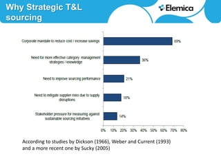
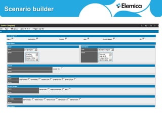
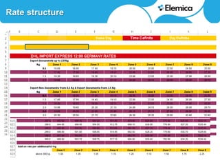
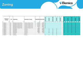
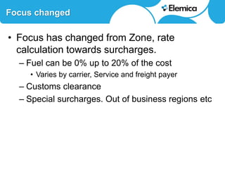
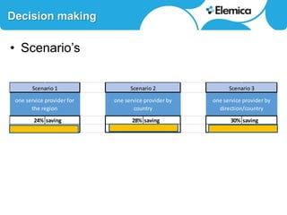
This document discusses optimizing transportation and logistics sourcing through strategic tendering. It recommends developing award scenarios upfront, knowing implementation costs, and focusing analyses on areas with the most potential gains. The best decisions balance current status with lowest cost while mitigating risks to quality, timeliness, and supply chain disruption. Historical data can provide insights into disturbances and reliability. Scenario modeling can quantify the financial impacts of objectives and constraints, like reducing carriers in a location. For small parcel shipping, the main players and their strong areas are identified. Rate structures have shifted from zones to more surcharges. Scenarios projecting 24-30% savings are presented based on consolidating carriers by region, country or direction. Reliability and

1. Elemica – T&L sourcing
Optimization

2. Why Strategic T&L
sourcing
According to studies by Dickson (1966), Weber and Current (1993)
and a more recent one by Sucky (2005)

3. Trend in T&L sourcing
• Tender complexity increases
– From local to regional tendering
– From service specific to
Network
• Increasing Supply chain
performance demands
– Transit time reliability
– Ability to absorb disruptions,
Alternative services and routings

4. Optimize your tendering
process
Speed up your decision process
• Develop awarding scenario’s
upfront and check after every
round where you are.
• Know your implementation cost
before you consider switching
suppliers.
• Reduce your workload during a
tender, focus only on those
area’s where you can gain.

5. Optimize your analyses
• Utilize your historical data to simulate the
cost of your future network with elements
such as:
– Weights/volumes.
– Peaks
– Routings
• Execute a sensitivity checks:
 currencies,
 fuel, e.d.

6. Optimize the decision
• Find the best between
• Current status and Cheapest pricing
• quality and timeliness
• Mitigate supplier risks to supply chain disruption
• Current and alternative performance (better or worse)
• Use the knowledge from your historical data.
• disturbances, reliability

7. We have a great tool
Our tool helps you to support these decisions.
• It evaluate the effects of your awarding scenario’s
with a baseline: What if you would stick to our
incumbents.
• Scenario’s are based on various constrains.
– It quantifies the financial impact your objectives
or constrains have.
• For example: reduce the nr carriers by location to 1.
– You compare the difference and measure it
against the effects to your supply chain.

8. Scenario builder

9. An example
Small parcels
• Small parcels
• Weight < 70 kg
• Dimensions:
Max hight = 60 cm
Max width = 60 cm
Max length = 120 cm
and 2* Hight + 2*width + length < 3 meter.
• Service
• World wide pick-up or delivery
• Express delivery before 9, 12 or end of day
• Expedited service (consolidation and slower
transport means)

10. Market
• Main players are
– UPS
– DHL
– Fedex
– TNT
– GLS
Each of these players have own “strong area’s”
where they are able to offer “domestic” small
parcel services.

11. Rate structure

12. Zoning

13. Zoning

14. Focus changed
• Focus has changed from Zone, rate
calculation towards surcharges.
– Fuel can be 0% up to 20% of the cost
• Varies by carrier, Service and freight payer
– Customs clearance
– Special surcharges. Out of business regions etc

15. Decision making
• Scenario’s
24% saving 28% saving 30% saving
Scenario 1 Scenario 2 Scenario 3
one service provider for
the region
one service provider by
country
one service provider by
direction/country
229,636 266,717 285,949

16. Where do we go to:
• We look for Reliability and quality of your
service providers. The data collected in the
Operating network provides you insight to
current strength and weaknesses of your
partners.
• Model probabilities on:
Carrier Transit times,
Seasonal effects
0
0.2
0.4
0.6
0.8
1
1.2
1 2 3 4 5 6
lane data distribution
of carrier 1 on lane 6
gamma distribution
(aplha=0.9, beta =2)