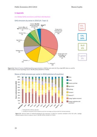
This document describes the use of modeling to analyze options for reducing greenhouse gas (GHG) emissions and their economic impacts. It discusses an accounting model called OPE2RA that was used to study scenarios for reducing Belgium's GHG emissions by 80-95% by 2050 compared to 1990 levels. The model establishes historical emissions by sector, builds baseline and mitigation scenarios by identifying reduction opportunities in sectors like transport, buildings, agriculture, industry and energy production, and analyzes scenario impacts on emissions, costs, energy use and other indicators.

1. Public
Economics
2013-­‐2014
Manon
Cuylits
Topic
5
:
Mitigation
options
“Reaching
80%
to
95%
GHG
emissions
reduction
[...]
is
possible.
Nevertheless,
reaching
this
target
is
very
challenging,
will
imply
large
reductions
in
all
sectors
and
a
thorough
understanding
of
the
various
interconnected
dimensions
is
key.”
Pestiaux
et
al.
(2013),
Scenarios
for
a
low
carbon
Belgium
by
2050,
Forthcoming
1.
Introduction
Objective
of
this
topic:
analyse
what
can
be
done
to
reduce
GHG
emissions
and
analyse
economic
impacts
of
these
actions
Models
are
used
to:
28
• Assess
the
emission
reduction
possibilities
at
the
level
of
a
sector/country/region/world
• Assess
the
impacts
of
emission
reductions
on
several
indicators
such
as
costs,
employment,
air
pollution,
etc...
This
requires
to
begin
with
a
clear
view
on:
• Possible
technological
levers
• Possible
behavioural
levers
• Their
combination
2.
Case-­‐study
on
Belgium
:
OPEERA
accounting
model
2.1.
Overall
approach
• Establish
historical
GHG
emissions
per
sector
(starting
point,
e.g.
2010)
• Establish
a
mid-­‐term
or
long-­‐term
“business-­‐as-­‐usual”
scenario
(e.g.
up
to
2020
or
2050),
i.e.
under
no
additional
policies/measures/actions,
to
be
used
as
a
benchmark/reference
against
which
the
impact
of
targets/policies/
actions
(levers)
are
to
be
assessed;
• In
each
(sub)sector,
identify
emission
reduction
levers
and
possible
ambition
levels
for
each
lever:
o Possible
technologies
aimed
at
reducing
GHG
emissions,
with
due
attention
to
the
level
of
deployment
(existing,
in
demonstration
phase,
in
R&D
phase,
...)
o Activity
levels,
such
as
travel
demand
per
person
or
industrial
production
• Build
scenarios,
i.e.
coherent
set
of
assumptions
and
levers
leading
to
required
level
of
total
emission
reductions
in
2050
• Analyse
the
impacts
of
each
scenario
on
e.g.
energy
security,
final
energy
demand,
costs,
etc...
Source:
Pestiaux
et
al.
(2013)

2. Public
Economics
2013-­‐2014
Manon
Cuylits
Main
question:
how
to
reduce
emissions
by
80
to
95%
by
2050
wrt
1990
and
what
are
the
main
impacts
of
such
large
reductions?
Historical
GHG
emissions
Belgium
has
reduced
its
emissions
by
~8%
since
1990
Historical
distribution
of
emissions
Emissions
in
2010
are
relatively
equally
distributed
between
power,
industry,
buildings
and
transport
29

3. Public
Economics
2013-­‐2014
Manon
Cuylits
Methodology
Based
on
open
and
transparent
tool
OPE2RA
developed
by
CLIMACT
and
VITO
on
the
basis
of
DECC
(UK)
pathways
calculator
Building
scenarios
2.2.
Sectoral
analysis
2.2.1.
Transport
Observations:
30
1. Transport
represents
about
a
quarter
of
the
overall
energy
consumption
in
Belgium
2. The
Belgian
motorized
transport
is
somewhat
less
car-­‐based
than
the
European
average
3. The
density
of
the
Belgian
highway
network
is
far
above
European
average
4. The
overall
distances
covered
by
passengers
since
1990
increased
by
30%,
cars
represent
~80%
5. Between
1990
and
2008,
cars
lost
some
share
to
buses
and
rail
transport
6. The
CO2
emissions
of
new
vehicles
have
been
decreasing
in
recent
years

4. Public
Economics
2013-­‐2014
Manon
Cuylits
31
7. Urbanization
levels
and
land
planning
play
a
crucial
role
in
GHG
mitigation
policies
8. The
availability
of
public
transport
influences
the
choice
of
transport
modes
9. The
Belgian
modal
split
for
goods
is
somewhat
less
road-­‐oriented
than
the
European
average
10. Road
transport
represents
the
bulk
of
energy
consumption
across
passenger
and
goods,
and
across
transport
modes
Levers
for
domestic
passenger
transport
(ambition
levels
1
and
4)

5. Public
Economics
2013-­‐2014
Manon
Cuylits
Visualisation
of
the
different
levels
of
technology
distribution
for
cars
Costs
:
capital
(CAPEX)
and
operational
(OPEX)
expenditures
in
2010
and
2050
–
Passenger
cars
32

6. Public
Economics
2013-­‐2014
Manon
Cuylits
Levers
for
freight
transport
(ambition
levels
1
and
4)
2.2.2.
Buildings
Levers
in
residential
buildings
include:
33
• for
heating:
compactness
of
buildings
(flats
vs
houses),
heating
comfort
level,
thermal
efficiency,
electrification
level,
innovative
heating
technologies;
• for
lighting
and
appliances:
demand/efficiency,
electrification

7. Public
Economics
2013-­‐2014
Manon
Cuylits
2.2.3.
Agriculture
Levers
include:
number
of
animals
and
meat
consumption,
emissions
intensity
per
animal
(enteric
fermentation
+
manure
management),
evolution
of
soil
emissions
2.2.4.
Industry
34

8. Public
Economics
2013-­‐2014
Manon
Cuylits
2.2.5.
Energy
production
(Energy
supply)
Levers
include
biomass,
geothermal,
wind
(onshore
and
offshore),
solar
PV,
solar
thermal,
Carbon
capture
and
sequestration
(CCS),
imports
of
electricity
2.3.
Scenarios
GHG
Emissions
Main
indicators
in
2050
35

9. Public
Economics
2013-­‐2014
Manon
Cuylits
2.4.
Costs
of
mitigation
scenarios
Undiscounted
costs
=>
does
not
assess
‘private
profitability’
of
investments
With
discounting
of
10%
(thus
rather
high
rate):
More
on
discounting
36
è
See
topic
8

10. Public
Economics
2013-­‐2014
Manon
Cuylits
2.5.
Build
and
assess
your
own
low
carbon
scenario
37
• UK:
http://2050-­‐calculator-­‐tool.decc.gov.uk
• BE:
forthcoming
on
www.climatechange.be/2050
• Walloon
region:
http://www.wbc2050.be
• China:
http://2050pathway-­‐en.chinaenergyoutlook.org
• Others
...
3.
Various
approaches
3.1.
Modelling
approaches
Accounting
models
(e.g.
OPE2RA,
SAVER-­‐LEAP,
EPM,
Anonymous
model
of
FPB)
• Central
modelling
logic:
to
guarantee
consistency
in
energy
accounting.
• Defining
activity
drivers
and
pathways
for
energy
efficiency
or
carbon
intensity
improvements
at
the
sectoral
levels
are
the
core
elements
of
the
methodology.
• Technologies
are
implicit
(no
‘production
function’)
and
costs
are
often
considered
in
an
ex-­‐post
calculation.
• The
particular
strength
of
accounting
models
is:
o Their
transparency
and
flexibility
in
presenting
energy
analysis
concepts
whilst
guaranteeing
consistency
in
energy
accounting.
o They
can
be
useful
to
explore
possible
pathways
and
provide
more
quantitative
analysis
on
the
required
targets
to
be
reached
by
the
underlying
hypothesis
at
sectoral
levels
o Can
be
useful
to
explore
the
social
acceptance
of
the
transition
as
well
as
its
contours
by
stakeholder
consultation
as
they
provide
powerful
reporting
capabilities.
Macro-­‐economic
models:
General
equilibrium
macro-­‐economic
model,
econometric
macro-­‐economic
models
(e.g.
GEM-­‐E3,
HERMES,
NEMESIS)
• Macroeconomic
models
represent
the
whole
economy
and
include
feedback
mechanisms
from
and
to
the
energy
system.
• These
models
are
based
on
the
same
type
of
behavioural
assumptions
for
the
economic
agents
but
they
differ
regarding
o the
market
equilibrium
assumptions
and
o the
dynamic
path
modelling.
• Econometric
models
are
more
oriented
towards
the
adjustment
path
in
the
short
to
medium
term
allowing
market
disequilibrium;
basis
is
:
Y
=
C
+I+G+X-­‐M
• General
equilibrium
model
are
medium
to
long
term
oriented
evaluating
the
impact
of
a
policy
when
the
full
effect
are
accounted
for;
based
on
maximisation
of
Utility
functions.
Partial
equilibrium
models
of
the
energy
system
(e.g.
TIMES
and
PRIMES)
• Have
a
detailed
representation
of
technologies
in
a
consistent
framework
• Partial
equilibrium
means
that
the
energy
demand
(curve)
is
fixed
(which
is
NOT
the
case
in
macroeconomic
models)
• PRIMES
and
TIMES
differ
in
their
mathematical
formulations:

11. Public
Economics
2013-­‐2014
Manon
Cuylits
38
o PRIMES
models
the
economic
agent’s
behaviour
(describing
what
would
happen
if);
this
takes
place
through,
a.o.
high
discount
rates
for
consumers
reflecting
some
form
of
information
failure
(private
discount
rate
=>
see
topic
8)
o TIMES
is
more
normative
from
the
point
of
view
of
the
public
authority
(prescribing
what
optimally
should
happen)
through,
a.o.
low
discount
rates
(close
to
social
discount
rate
=>
see
topic
8)
• Example:
on
blackboard
Trade-­‐offs
3.2.
What
do
we
mean
by
«
costs
»
?
Macroeconomic
models:
GDP
and/or
welfare:
• Macroeconom(étr)ic
models
and
some
CGE
models,
i.e.
required
feedback
of,
typically,
changes
in
energy
system
on
the
whole
economy,
including
public
sector
(taxes,
revenues,
...)
• Thus
level
of
economic
activity
(GDP),
also
per
sector,
employment
effects,
possibly
competitiveness,
...
• Computable
general
equilibrium
(CGE)
models,
i.e.
based
on
utility
function,
thus
relative
change
in
Utility
(%)
is
computed
Partial
equilibrium
models:
energy
system
including
loss
of
consumer
surplus:
• Costs
of
technologies
• Possibly,
loss
of
consumer
surplus
Accounting
models:
energy
system
costs:
Capex
–
Opex
–
Fuel
Other
important
costs
(or
benefits)
are
usually
not
included
in
models
and
must
be
computed
separately:
health
effects
of
changes
in
emissions,
energy
security,
traffic
congestion,
...

12. Public
Economics
2013-­‐2014
Manon
Cuylits
4.
Appendix
A.1
Global
GHG
emissions
and
their
distribution
GHG
emissions
by
sector
in
2010
(cfr.
Topic
1)
Shares
of
GHG
emissions
per
sector
in
2010
(selection
of
countries)
39

13. Public
Economics
2013-­‐2014
Manon
Cuylits
A.2
What
are
negative
emissions?
Negative
emissions
IPCC
scenarios
to
keep
temperature
rise
below
2°C
indicate
that
it
might
be
required
to
reduce
emissions
below
0
(i.e.
net
absorption
of
carbon
dioxide).
What
are
negative
emissions?
IEA
(2013),
Box
1.1,
p.17:
Readings
40
• Pestiaux,
J.,
Cornet,
M.,
Duerinck,
J.,
Laes,
E.,
Lodewijks,
P.,
Meynaerts,
E.,
Renders,
N.
and
Vermeulen,
P.
(2013),
Scenarios
for
a
low
carbon
Belgium
by
2050,
Final
Report,
Study
performed
for
the
Climate
Change
Section
of
the
Federal
Public
Service
Health,
Food
Chain
Saftey
and
Environment,
forthcoming
(www.climatechange.be/2050)
• IEA
(2013),
Redrawing
the
energy-­‐climate
map,
World
Energy
Outlook
Special
Report.
• Duerinck,
J.
(2012),
Transition
towards
a
low
carbon
society
in
2050:
Status
of
long
term
modelling
in
Belgium,
Mimeo
(forthcoming
on
www.climatechange.be/2050)