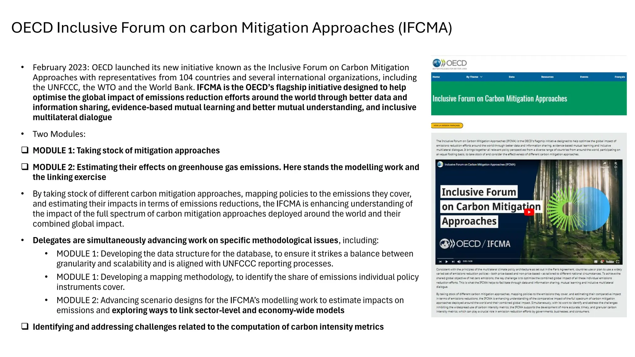
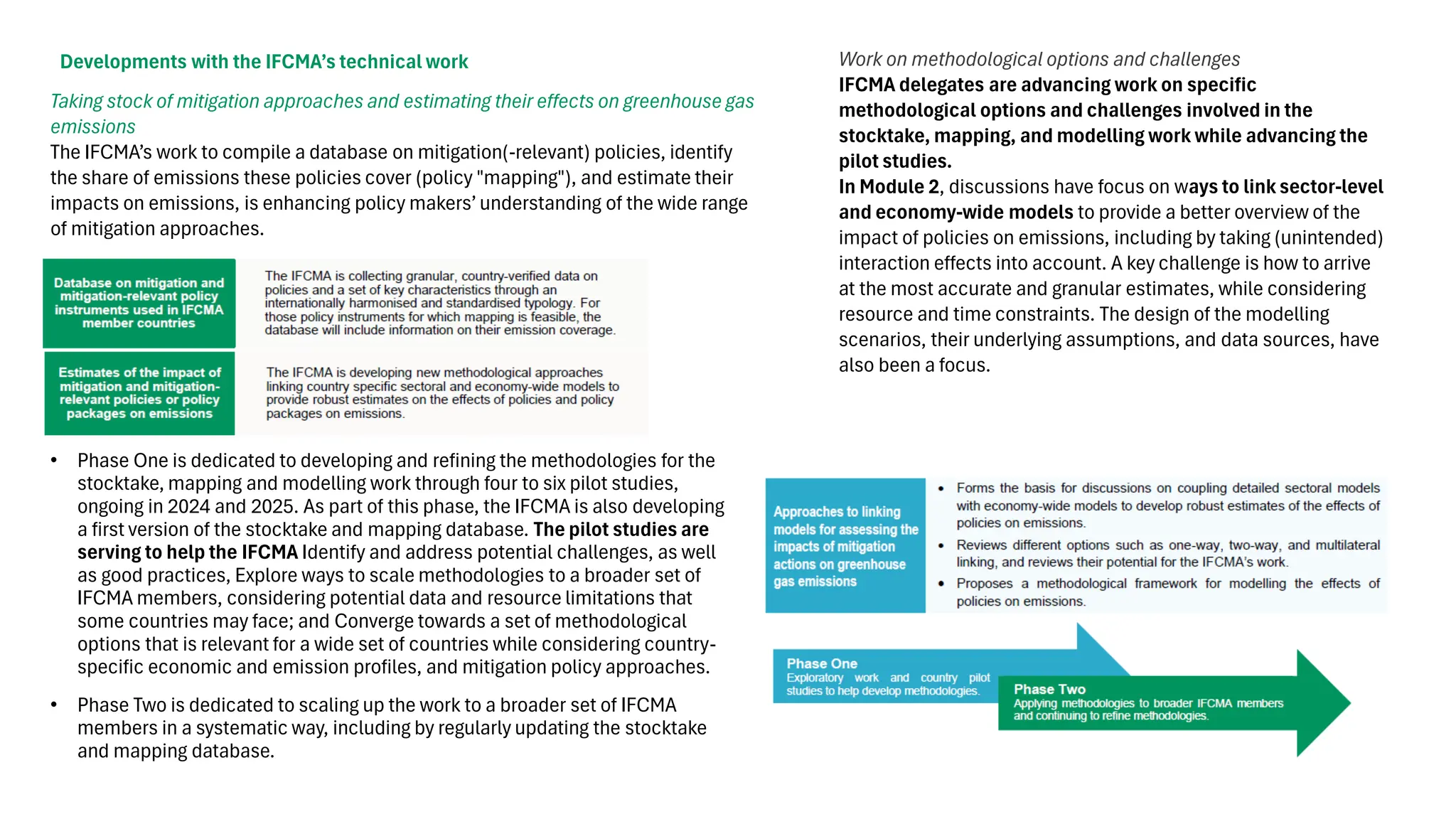
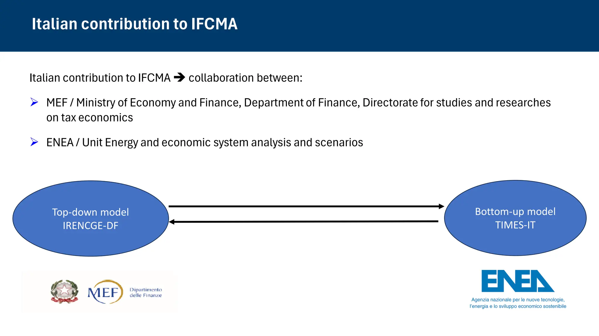
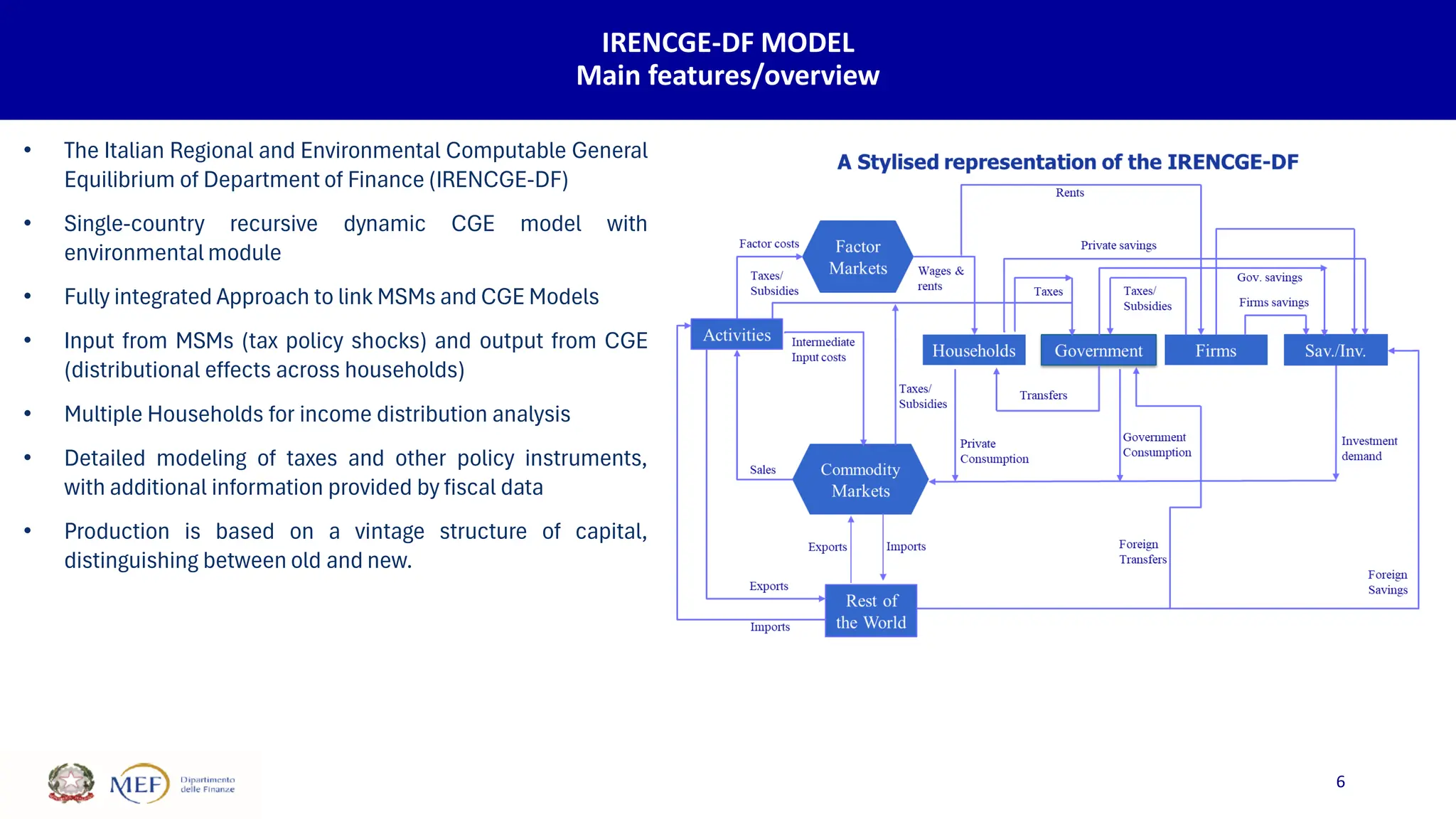
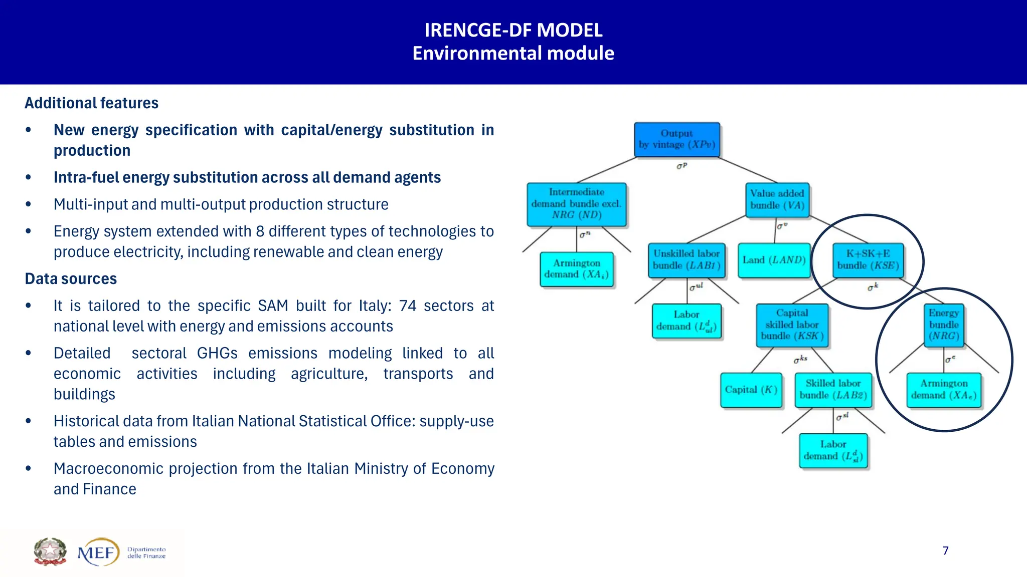
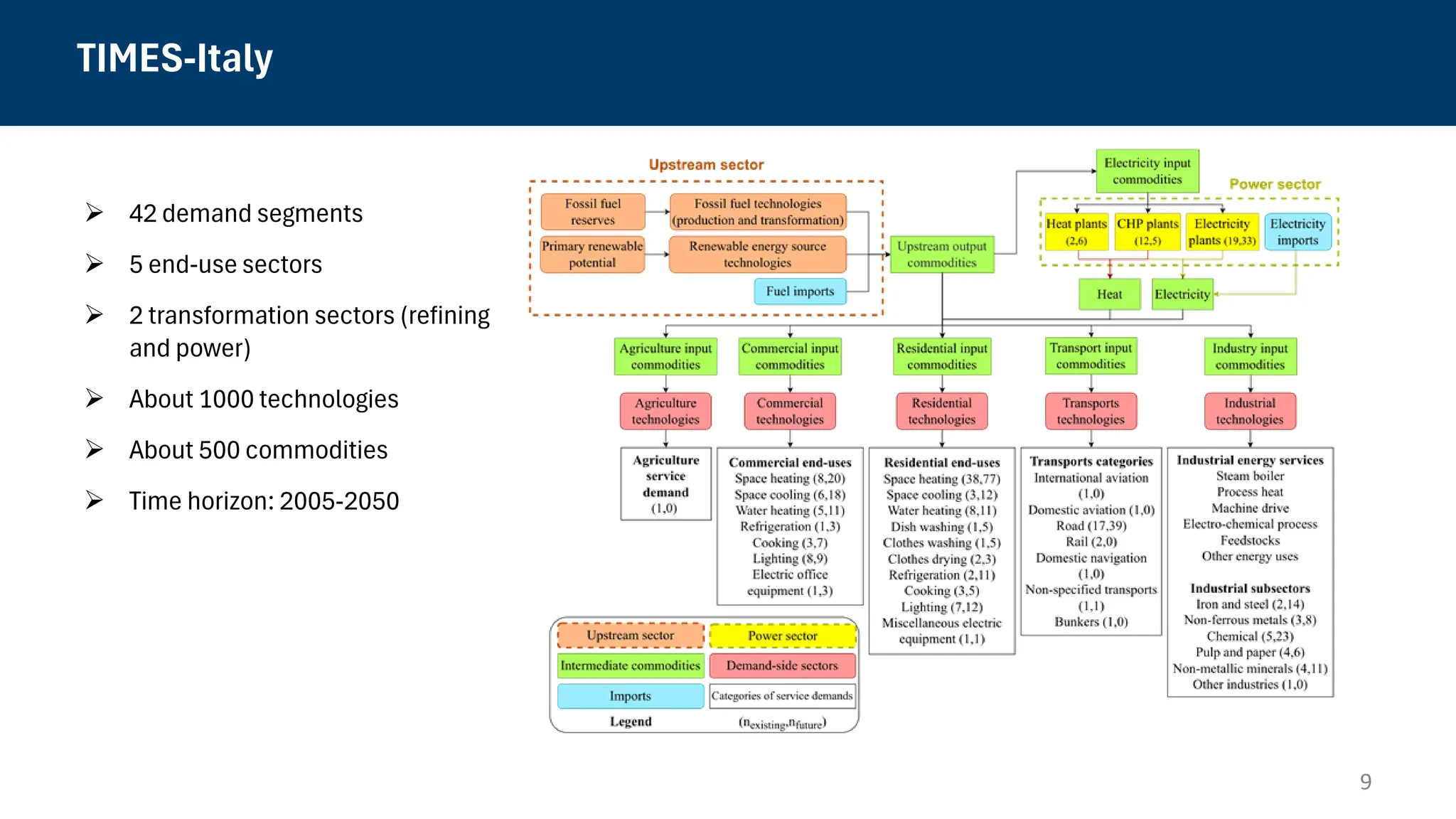
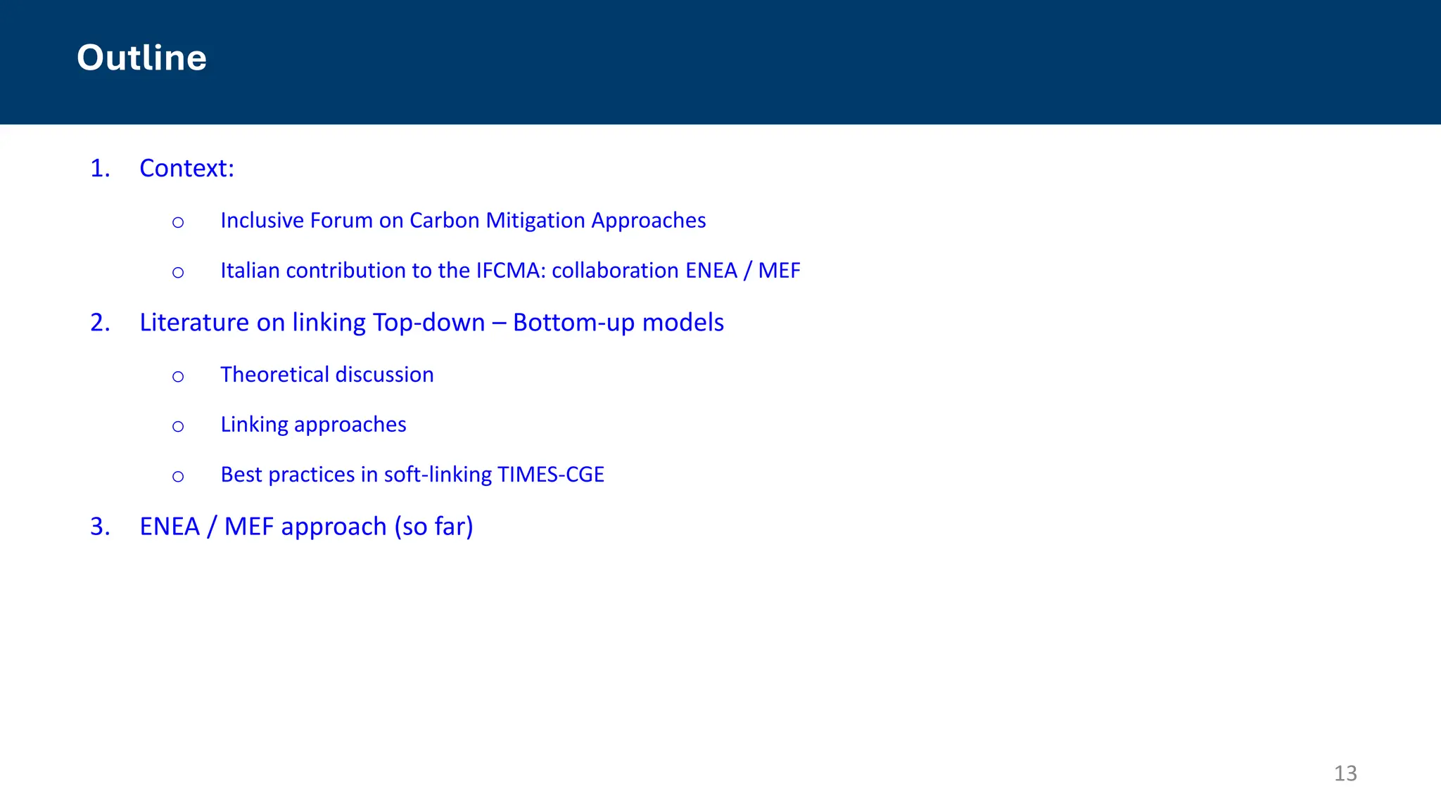
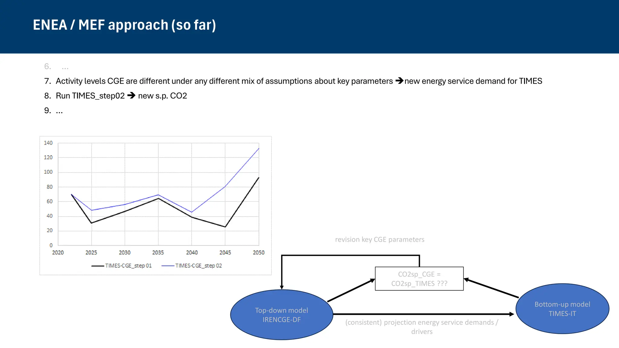
The document discusses the collaboration between ENEA and the Ministry of Economy and Finance (MEF) in Italy to contribute to the OECD's Inclusive Forum on Carbon Mitigation Approaches (IFCMA). It focuses on integrating top-down (CGE) and bottom-up (TIMES) models to enhance the understanding of carbon mitigation policies and their impact on greenhouse gas emissions through a refined methodology. Key phases involve pilot studies, data harmonization, and scenario analyses to model decarbonization pathways towards achieving net-zero emissions by 2050.

1. Combined use of TIMES and CGE models to explore methodological issues
related to the economic implication of decarbonization pathways
Francesco Gracceva, Bruno Baldissara, Vittoria Battaglia, Livio De Chicchis, Daniela Palma (ENEA)
Gionata Castaldi, Marco Manzo, Maria Teresa Monteduro, Carlo Orecchia, Vera Santomartino (Ministry of Economy and Finance)
ETSAP workshop, Bonn, 24/06/2024

2. 1. Context:
o Inclusive Forum on Carbon Mitigation Approaches
o Italian contribution to the IFCMA: collaboration ENEA / MEF
2. Literature on linking Top-down – Bottom-up models
o Theoretical discussion
o Linking approaches
o Best practices in soft-linking TIMES-CGE
3. ENEA / MEF approach (so far)
2
Outline

3. OECD Inclusive Forum on carbon Mitigation Approaches (IFCMA)
• February 2023: OECD launched its new initiative known as the Inclusive Forum on Carbon Mitigation
Approaches with representatives from 104 countries and several international organizations, including
the UNFCCC, the WTO and the World Bank. IFCMA is the OECD’s flagship initiativedesigned to help
optimise the global impact of emissions reduction efforts around the world through better data and
information sharing, evidence-based mutual learning and better mutual understanding, and inclusive
multilateral dialogue
• Two Modules:
❑ MODULE 1: Taking stock of mitigation approaches
❑ MODULE 2: Estimating their effects on greenhouse gas emissions. Here stands the modelling work and
the linking exercise
• By taking stock of different carbon mitigation approaches, mapping policies to the emissions they cover,
and estimating their impacts in terms of emissions reductions, the IFCMA is enhancing understanding of
the impact of the full spectrum of carbon mitigation approaches deployed around the world and their
combined global impact.
• Delegates are simultaneously advancing work on specific methodological issues, including:
• MODULE 1: Developing the data structurefor the database, to ensure it strikes a balance between
granularity and scalability and is aligned with UNFCCC reporting processes.
• MODULE 1: Developing a mapping methodology, to identify the share of emissions individual policy
instruments cover.
• MODULE 2: Advancing scenario designs for the IFCMA’s modelling work to estimate impacts on
emissions and exploring ways to link sector-level and economy-wide models
❑ Identifying and addressing challenges related to the computation of carbon intensity metrics

4. • Phase One is dedicated to developing and refining the methodologies for the
stocktake, mapping and modelling work through four to six pilot studies,
ongoing in 2024 and 2025. As part of this phase, the IFCMA is also developing
a first version of the stocktake and mapping database. The pilot studies are
serving to help the IFCMA Identify and address potential challenges, as well
as good practices, Explore ways to scale methodologies to a broader set of
IFCMA members, considering potential data and resource limitations that
some countries may face; and Converge towards a set of methodological
options that is relevant for a wide set of countries while considering country-
specific economic and emission profiles, and mitigation policy approaches.
• Phase Two is dedicated to scaling up the work to a broader set of IFCMA
members in a systematic way, including by regularly updating the stocktake
and mapping database.
Developments with the IFCMA’s technical work Work on methodological options and challenges
IFCMA delegates are advancing work on specific
methodological options and challenges involved in the
stocktake, mapping, and modelling work while advancing the
pilot studies.
In Module 2, discussions have focus on ways to link sector-level
and economy-wide models to provide a better overview of the
impact of policies on emissions, including by taking (unintended)
interaction effects into account. A key challenge is how to arrive
at the most accurate and granular estimates, while considering
resource and time constraints. The design of the modelling
scenarios, their underlying assumptions, and data sources, have
also been a focus.
Taking stock of mitigation approaches and estimating their effects on greenhouse gas
emissions
The IFCMA’s work to compile a database on mitigation(-relevant) policies, identify
the share of emissions these policies cover (policy "mapping"), and estimate their
impacts on emissions, is enhancing policy makers’ understanding of the wide range
of mitigation approaches.

5. Top-down model
IRENCGE-DF
Bottom-up model
TIMES-IT
Italian contribution to IFCMA
Italian contribution to IFCMA ➔ collaboration between:
➢ MEF / Ministry of Economy and Finance, Department of Finance, Directorate for studies and researches
on tax economics
➢ ENEA / Unit Energy and economic system analysis and scenarios

6. 6
IRENCGE-DF MODEL
Main features/overview
• The Italian Regional and Environmental Computable General
Equilibrium of Department of Finance (IRENCGE-DF)
• Single-country recursive dynamic CGE model with
environmental module
• Fully integrated Approach to link MSMs and CGE Models
• Input from MSMs (tax policy shocks) and output from CGE
(distributional effects across households)
• Multiple Households for income distribution analysis
• Detailed modeling of taxes and other policy instruments,
with additional information provided by fiscal data
• Production is based on a vintage structure of capital,
distinguishing between old and new.

7. 7
IRENCGE-DF MODEL
Environmental module
Additional features
• New energy specification with capital/energy substitution in
production
• Intra-fuel energy substitution across all demand agents
• Multi-input and multi-output production structure
• Energy system extended with 8 different types of technologies to
produce electricity, including renewable and clean energy
Data sources
• It is tailored to the specific SAM built for Italy: 74 sectors at
national level with energy and emissions accounts
• Detailed sectoral GHGs emissions modeling linked to all
economic activities including agriculture, transports and
buildings
• Historical data from Italian National Statistical Office: supply-use
tables and emissions
• Macroeconomic projection from the Italian Ministry of Economy
and Finance

8. 8
Modelling the carbon pricing impacts
Carbon pricing affects the economy through 4 channels
1
2
3
4
Expenditure channel (Modelled)
• Higher price of fuels and goods that use fuel as an input --> incentive for firms and households
to substitute emission intensive inputs and commodities with more sustainable alternatives
Revenue recycling channel (Modelled)
• Impact of revenue uses, including cash transfers, tax reductions, public investment, budget
support, incentives for private investments etc.
Income channel (Modelled)
• Impacts on labor market and factor income: as inputs costs raise, production decreases,
inducing a reduction in wages and rents, reducing households income
Health co-benefits channel (Modelled but not yet simulated)
• Low-income households have higher exposure to local pollutants

9. TIMES-Italy
➢ 42 demand segments
➢ 5 end-use sectors
➢ 2 transformation sectors (refining
and power)
➢ About 1000 technologies
➢ About 500 commodities
➢ Time horizon: 2005-2050
9

10. Low-carbon options modules
Hydrogen module CCS module

11. A scenario analysis on Net Zero Italy by 2050
18 alternative pathways to achieve complete decarbonization by 2050, built
by combining different assumptions about
• future evolution of the energy service demand to be satisfied (high,
medium, low) and
• actual deployment of a set of low-carbon energy technology clusters. i.e.
low-carbon dispatchable electricity, biofuels, hydrogen and synthetic
fuels
Aim: to assess whether Net-Zero is
• technically feasible
• how challenging it is to achieve it
• what its additional costs are
Key messages:
• 2030 target set in the EU Fit55 + Net Zero 2050 is technically feasible
• But the path is narrow: a necessary condition is that all the main
innovative low-carbon technologies have a “optimistic” evolution.
• While in the event of a pessimistic evolution of even just one of the main
low-carbon technology clusters, hydrogen included, NZ 2050 is not
achievable 11
Storyline socio-economica
nome caso descrizione
Dynamics-as-
usual
Low energy
service intensity
& fast LCT
Energy
intensive
lifestyle
Ipotesi
su
evoluzione
tecnologie
low-carbon
Net
Zero_Reference
Low carbon tech. tutte
disponibili / ip. ottimistiche
√ √ X
Net Zero_Solo
FRNP
no CCS, sviluppo limitato di
H2 e biomasse
X X X
Net Zero_FRNP-
Ip. meno ottimistiche sul
potenziale Fonti Rinnovabili
Non Programmabili
X √ X
Net Zero_noLC
baseload
Indisponibilità di impianti di
generazione baseload a
basse/nulle emissioni
X ≈ X
Net Zero_H2-
Costi elevati tecnologie
dell'idrogeno
X ≈ X
Net Zero_Bio-
Ip. meno ottimistiche sul
potenziale Biomasse
X √ X

12. Net Zero Italy by 2050
12
2002 2012
2022 2050
0
500
1000
1500
2000
2500
3000
3500
-50% -55% -60% -65% -70% -75% -80% -85% -90% -95%
Costo
marginale
abbattim.
(€/t)
% riduzione CO2 nel 2050 vs 2005
Traiettoria socio-economica Base Traiettoria meno energivora
Marginal abatement cost curve

13. 1. Context:
o Inclusive Forum on Carbon Mitigation Approaches
o Italian contribution to the IFCMA: collaboration ENEA / MEF
2. Literature on linking Top-down – Bottom-up models
o Theoretical discussion
o Linking approaches
o Best practices in soft-linking TIMES-CGE
3. ENEA / MEF approach (so far)
13
Outline

14. (fonte: Encyclopedia of Energy, Elsevier, 2004)
The first modeling efforts investigating the relationships between
energy and economics date back to the 1970s. Since the
beginning, two broad classes of modeling approaches
appeared:
• The economic or top-down models, adopting a general
perspective, described the economic linkages between
energy demand and supply and the rest of the economic
system, with the main goal of analyzing energy or wider
economic policies.
• The technical/engineering or bottom-up models,
adopting a focused view of the energy sectors, explored
the various technological options, with the main goal of
highlighting low-cost energy production opportunities
• Top Down ➔ «past can describe the future»
• Bottom Up ➔ “the future is changeable”
Top-down vs Bottom-up

15. Top-down vs Bottom-up
• Top-down models, with their descriptions of feedback effects in the total economy but fewer technical details on the energy system
studies “tend to underestimate the potential for low-cost efficiency improvements (and overestimate abatement costs) because
they ignore a whole category of gains that could be tapped by nonprice policy changes”
• Bottom-up engineering models, ignoring feedbacks to the general economy and non technicalmarket factors but containing rich
descriptions of technology options “overestimate the potential (and underestimate abatement costs) because they neglect various
"hidden" costs and constraints that limit the uptake of apparently cost-effective technologies”
• Or the principal difference may be that the engineering models ignore new sources of energy demands, and that the macroeconomic
models ignore“saturation effects”, that is, the decoupling of demand growth from that of GDP (Kram, 1993)
• the reason why they typically produce substantially different results, e.g. in terms of the abatement costs associated to a specific
policy scenario, is because“they reflect very different perspectives, almost paradigms, about driving forces in the energy economy”.
As such,“these two ways of seeing and describing the world are conceptually incompatible”, therefore“one cannot expect their
models to produce compatible results by simply adjusting the numbers”.
➔ Which is more "realistic" (…) cannot be determined without separate study of specific implementation policies and costs. (…) But we
can say with some confidence that the real near-term potential for limiting CO2 emissions at low or negative costs lies somewhere
between the optimism of such bottom-up studies, and the relative pessimism of many top-down studies

16. Linking approaches
• In a one-way linkage, outputs from one model serve as exogenous parameters or variables in another model. Consistency is generally not
achieved
• two-way linkage takes into account the feedback between models to reach better convergence of overlapping variables. As exemplified
for CGE-PE energy model linking in Figure 1, the energy supply structure and cost from a PE energy model is used to inform a CGE model
to modify the energy demand structure in the CGE model that is fed back into the energy supply model. Therefore the two-way linkage
provides better convergence between the linked models for both energy supply and demand variables.
• Several methodological challenges: deal with differences in model scope and resolution as well as modeling concepts and related
underlying (implicit) assumptions, … sector definitions and energy supply/demand structure differ across models➔ need for translation
modules (e.g. to translate sector production activity from CGE into the energy demand drivers used in the bottom-up model)
Journal of Global Economic Analysis, Volume 5 (2020), No. 1, pp. 162-195.

17. Best practice soft-linking involving TIMES models
National soft-linking: ‘full-link’ and ‘full-
form’ approach
• Labriet et al. (2010), Fortes et al.
(2014), Dai et al. (2016), Krook-
Riekkola et al. (2017), Timilsina
(2021)
• Anderson et al. (2019)
• CGE ➔ sectoral energy service
demands drivers used in the
bottom-up energy system
optimization
• energy system bu model (TIMES) ➔
to inform a national CGE model on
how sectoral fuel mix and fuel
efficiency changes over time
• Best-practice linkage approaches
aim at minimal differences in
endogenous variables simulated by
both models and at harmonized
exogenous assumptions driving the
linked models

18. Philosophy soft-link methodologies
Underlying assumption ➔ CGE models are considered unable to explicitly
address aspects of the energy system related to
• (i) changes in energy intensity due to introduction of new technologies
• (ii) changes in the energy mix following changes in energy demand
• (iii) changes in electricity and heating prices due to competition of limited
energy commodities between and within sectors
➔ Information from BU to TD ➔ TD is constrained to reproduce the
evolution of the energy system depicted by BU, by
- Adjusting AEEI
- Changing production function (to Leontief type)
- …
BUT we know that:
• BU too optimistic, lack of behavioural realism
• BU too flexible, technologies as perfect substitutes, winner takes all
• BU lack endogenous market adjustments (no demand reduction after a
carbon constraint) ➔ prices increase more than in reality
➢ “A challenge and source of uncertainty in soft-linking hybrid
models is the price information from bottom up optimisation
models to top down models. The price change between the base
year and the end of horizon year are found to be exaggerated.
The main explanation for this is that the calculated prices in the
first modelling years do not include all costs” (Krook et al.)
➔ QUESTION:
- Is it the best choice to lose information coming from TD about the
flexibility of the system?
• Linking model aims at exploiting their complementary strengths, to benefit from the technological details provided by BU and the assessment of the
interactions between the energy system and the economy provided by CGE
• Predominant philosophy (?) soft-linking methodologies: to integrate the simplified description of the energy system included in CGE models with information
coming from bottom-up models (up to fully constraining CGE to reproduce the results of energy models)

19. 1. Context:
o Inclusive Forum on Carbon Mitigation Approaches
o Italian contribution to the IFCMA: collaboration ENEA / MEF
2. Literature on linking Top-down – Bottom-up models
o Theoretical discussion
o Linking approaches
o Best practices in soft-linking TIMES-CGE
3. ENEA / MEF approach (so far)
19
Outline

20. ENEA / MEF approach (so far)
1. Harmonization two models wrt main exogenous assumptions: population, import prices, baseline emissions profile
2. First run of two models separately
➢ check consistency base year data
➢ fix unrealistic TD results (e.g. hydro)
➢ assess capability to reproduce historical years (under historical evolution exogenous drivers)
IRENCGE-DF TIMES-IT

21. Top-down model
IRENCGE-DF
Bottom-up model
TIMES-IT
1. Harmonization two models wrt main exogenous assumptions: population, import prices, baseline emissions profile
2. First run two models separately
3. Run CGE_Baseline (incl. Baseline CO2 emission profile or Carbon price, from NECP)
4. TD to BU linking ➔ (consistent) projection of energy service demand or demand drivers ➔ input to TIMES
5. Run TIMES-It_Baseline (incl. Baseline CO2 emissions profile or Carbon price, from NECP) with revised energy service demand
➔ Connection point: CO2 shadow price in target year (or emission profile) similar in two models similar flexibility
6. CO2 Shadow price (or emissions profile) ➔ comparison BU vs TD ➔ IF different ➔ key CGE parameters (AEEI, ESUB, …) adjusted so that
CGE CO2 shadow price (or emissions profile) is similar to TIMES CO2 s.p.
7. Activity levels CGE are different under any different mix of assumptions about key parameters ➔new energy service demand for TIMES
8. Run TIMES_step02 ➔ new s.p. CO2
(consistent) projection energy service demands / drivers
CO2sp_CGE = CO2sp_TIMES ???
revision key CGE parameters
ENEA / MEF approach (so far)

22. electrification AEEI
sigma
KLEM
sigma
(interfuel
esub)
sigma
export
sigma
import
carbon
price
emissions
2050
(GHG)
emissions
2050 (CO2)
1 no shocks no shocks 0,2 0,25 3 2 infes. 2045 291 231
2 no shocks no shocks 0,2 0,5 3 2 335 291 231
3 no shocks no shocks 0,5 0,5 3 2 310 291 231
4 no shocks no shocks 0,8 0,5 3 2 288 291 231
5 no shocks 10% in 2050 0,8 0,5 3 2 253 291 231
6 no shocks 30% in 2050 0,8 0,5 3 2 206 291 231
7 no shocks 40% in 2050 0,8 0,5 3 2 190 291 231
7bis no shocks 40% in 2050 0,9 0,5 3 2 196 291 231
7ter no shocks 40% in 2050 2 0,5 3 2 241 291 231
8 no shocks 40% in 2050 0,8 0,8 1,5 1,2 166 291 231
9 no shocks 40% in 2050 0,8 1,2 1,5 1,2 150 291 231
10 no shocks 40% in 2050 0,8 2 1,5 1,2 128 291 231
?? ?? ?? ?? 90 291 231
11 no shocks no shocks 0,2 0,25 3 2 90 infeasible
12 no shocks no shocks 0,2 0,5 3 2 90 430 341
13 no shocks no shocks 0,5 0,5 3 2 90 406 322
14 no shocks no shocks 0,8 0,5 3 2 90 412 327
15 no shocks 10% in 2050 0,8 0,5 3 2 90 399 317
16 no shocks 30% in 2050 0,8 0,5 3 2 90 378 300
17 no shocks 40% in 2050 0,8 0,5 3 2 90 370 294
17bis no shocks 40% in 2050 0,9 0,5 3 2 90 378 300
17ter no shocks 40% in 2050 2 0,5 3 2 90 474 376
18 no shocks 40% in 2050 0,8 0,8 1,5 1,2 90 352 279
19 no shocks 40% in 2050 0,8 1,2 1,5 1,2 90 345 274
20 no shocks 40% in 2050 0,8 2 1,5 1,2 90 infeasible
Baseline CO2 PRICE (from NECP)
Baseline CO2 EMISSIONS PROFILE (from NECP)
We began with low substitutability between capital, labor, and energy
(KLEM), gradually increasing it from 0.2 up to 0.8.
• This change resulted in a decrease in the carbon price (i.e., the
marginal abatement cost) from 335 to 288 EUR/TCO2e by 2050.
Subsequently, we increased energy efficiency (AEEI shifters) gradually
by 10%, reaching up to a 40% improvement by 2050 (equating to
approximately a 1% yearly increase).
• The combined increase in KLEM substitutability and AEEI resulted
in a further reduction of the carbon price to 190 EUR/TCO2e.
• However, further increasing KLEM substitutability to 2 led to
significant rebound and leakage effects, primarily through
increased imports of electricity and other energy-intensive
products, causing the carbon price to rise to 241 EUR/TCO2e.
• By reducing the trade Armington elasticities (from 2 to 1.2 and from
3 to 1.5), we effectively reduced the abatement effort needed to
maintain the imposed emission cap. This adjustment further
decreased the carbon price to 128 EUR/TCO2e.
• It is important to note that model convergence problems can arise
if assumptions, such as KLEM or intrafuel energy substitutability
and energy efficiency improvements, are set too high.
ENEA / MEF approach (so far)

23. Top-down model
IRENCGE-DF
Bottom-up model
TIMES-IT
6. …
7. Activity levels CGE are different under any different mix of assumptions about key parameters ➔new energy service demand for TIMES
8. Run TIMES_step02 ➔ new s.p. CO2
9. …
(consistent) projection energy service demands /
drivers
CO2sp_CGE =
CO2sp_TIMES ???
revision key CGE parameters
ENEA / MEF approach (so far)